Exact solutions of Lovelock-Born-Infeld Black Holes

Abstract

The exact five-dimensional charged black hole solution in Lovelock gravity coupled to Born-Infeld electrodynamics is presented. This solution interpolates between the Hoffmann black hole for the Einstein-Born-Infeld theory and other solutions in the Lovelock theory previously studied in the literature. The conical singularity of the metric around the origin can be removed by a proper choice of the black hole parameters. The thermodynamical properties of the solution are also analyzed and, in particular, it is shown that the behaviour of the specific heat indicates the existence of a stability transition point in the vacuum solutions. We discuss the similarities existing between this five-dimensional geometry and the three-dimensional black hole. Like BTZ black hole, the Lovelock black hole has an infinite lifetime.

I Introduction

The Einstein tensor is the only symmetric and conserved tensor depending on the metric and its derivatives up to the second order, which is linear in the second derivatives of the metric. Dropping the last condition, Lovelock lovelock (1) found the most general tensor satisfying the other ones. The obtained tensor is non linear in the Riemann tensor and differs from the Einstein tensor only if the space-time has more than 4 dimensions. Therefore the Lovelock theory is the most natural extension of general relativity in higher dimensional space-times. The Lovelock theory for a particular choice of the coefficients of the action could be thought as the gravitational analogue of Born-Infeld electrodynamics ban (2).

In the last decades a renewed interest in both Lovelock gravity and Born-Infeld electrodynamics has appeared because they emerge in the low energy limit of string theory frad (3, 4, 5). Since the Lovelock tensor contains derivatives of the metric of order not higher than the second, the quantization of the linearized Lovelock theory is free of ghosts. For this reason the Lovelock Lagrangian appears in the low energy limit of string theory. In particular, the Gauss-Bonnet terms (quadratic in the Riemann tensor) were studied in Ref. zwi (6) and the quartic terms in Refs. cai (7, 8). The Lovelock theory of gravity was also discussed in Refs. joel (9, 10, 11).

Hoffmann was the first one in relating general relativity and the Born-Infeld electromagnetic field Hoffmann (12). He obtained a solution of the Einstein equations for a point-like Born-Infeld charge, which is devoid of the divergence of the metric at the origin that characterizes the Reissner-Nordström solution. However, a conical singularity remained there, as it was later objected by Einstein and Rosen. The Einstein-Born-Infeld black hole has been revisited in Refs. gibb (14, 15)

The aim of this paper is to study the charged black hole solutions in five-dimensional Lovelock gravity coupled to Born-Infeld electrodynamics. In section II, we discuss the five-dimensional Lovelock gravity and study the black hole solutions as a preliminary step toward the calculation of the charged solution which we present in a separated section. In section III, we discuss the Born-Infeld electrodynamics which will provide us the necessary tools in order to eventually find, in section IV, the five- dimensional charged black hole solution in Lovelock-Born-Infeld field theory. We study the geometrical properties of the solution and discuss the similarities and distinctions existing with respect to the Reissner-Nordström black hole. Section V is dedicated to the analysis of the thermodynamics of the Lovelock black holes and the conclusions are contained in section VI.

II Lovelock theory

The Lovelock Lagrangian density in $D$ dimensions is lovelock (1, 16)

$${\cal L}=\sum_{k=0}^{N}\alpha_{k}\>\lambda^{2(k-1)}\>{\cal L}_{k}$$ (1)

where $N=\frac{D}{2}-1$ (for even $D$) and $N=\frac{D-1}{2}$ (for odd $D$). In (1), $\alpha_{k}$ and $\lambda$ are constants which represent the coupling of the terms in the whole Lagrangian and give the proper dimensions.

In Eq. (1) ${\cal L}_{k}$ is

$${\cal L}_{k}=\frac{1}{2^{k}}\sqrt{-g}\>\delta^{i_{1}...i_{2k}}_{j_{1}...j_{2k}}\>R^{j_{1}j_{2}}_{i_{1}i_{2}}...\>R^{j_{2k-1}j_{2k}}_{i_{2k-1}i_{2k}}$$ (2)

where ${R^{\mu}\>_{\nu\rho\gamma}}$ is the Riemann tensor in $D$ dimensions, $R^{\mu\nu}\>_{\rho\sigma}=g^{\nu\delta}\>R^{\mu}\>_{\delta\rho\sigma}$, $g$ is the determinant of the metric $g_{\mu\nu}$ and $\delta^{i_{1}...i_{2k}}_{j_{1}...j_{2k}}$ is the generalized Kronecker delta of order $2k$ grav (17).

The Lagrangians up to order 2 are given by deru (16, 18, 19)

${\cal L}_{0}=\sqrt{-g}$

${\cal L}_{1}=\frac{1}{2}\>\sqrt{-g}\>\delta^{i_{1}i_{2}}_{j_{1}j_{2}}\>R^{j_{1}j_{2}}_{i_{1}i_{2}}=\sqrt{-g}\>R\;\;\;$

${\cal L}_{2}=\frac{1}{4}\>\sqrt{-g}\>\delta^{i_{1}i_{2}i_{3}i_{4}}_{j_{1}j_{2}j_{3}j_{4}}\>R^{j_{1}j_{2}}_{i_{1}i_{2}}\>R^{j_{3}j_{4}}_{i_{3}i_{4}}=\;\>\>$

$$\;\;=\sqrt{-g}\>(R_{\mu\nu\rho\sigma}\>R^{\mu\nu\rho\sigma}-4\>R_{\mu\nu}\>R^{\mu\nu}+R^{2})$$

where we recognize the usual Lagrangian for the cosmological term, the Einstein-Hilbert Lagrangian and the Lanczos Lagrangian lan (18, 19) respectively.

For dimensions $D=5$ and $D=6$ the Lovelock Lagrangian is a linear combination of the Einstein-Hilbert and Lanczos Lagrangians. The spaces of dimensions $D=7$ and $D=8$ includes the Lagrangian ${\cal L}_{3}$, which was first obtained by Müller-Hoissen mul (20). In general, if the dimension is even and the manifold is compact with positive definite metric, then ${\cal L}_{D/2}$ is the Euler characteristic classes generator pat (21)

$$\int_{\mho}\>d^{2n}x\>{\cal L}_{n}=\frac{(-1)^{n+1}\>2^{2+n}\>\pi^{n}\>n!}{(2n)!}\chi(\mho)$$

where $\chi(\mho)$ are the Euler-Poincaré topological invariants, which are zero in odd dimensions.

Hence, the geometric action is written as

$$S=\int d^{D}x\>{\cal L}$$ (3)

From the variational principle we obtain the Lovelock tensor (${\cal G}_{\mu\nu}$),

$$\delta S=\int d^{D}x\>\delta{\cal L}=\int d^{D}x\>{\cal G}_{\mu\nu}\>\sqrt{-g}\>\delta g^{\mu\nu}$$ (4)

where the general expression of ${\cal G}_{\mu\nu}$ is lovelock (1, 22)

$${\cal G}^{\mu}\>_{\nu}(k)=-\frac{1}{2^{k+1}}\>\delta_{\nu\>j_{1}j_{2}....j_{2k}}^{\mu\>i_{1}i_{2}....i_{2k}}\>R^{j_{1}j_{2}}_{i_{1}i_{2}}\>....R^{j_{2k-1}j_{2k}}_{i_{2k-1}i_{2k}}$$ (5)

$${\cal G}_{\mu\nu}=\sum_{k=0}^{N}\alpha_{k}\>\lambda^{2(k-1)}\>{\cal G}_{\mu\nu}(k)$$ (6)

where $N=\frac{D}{2}-1$ for even $D$ or $N=\frac{D-1}{2}$ for odd $D$. When the dimension is $D=4$, ${\cal G}_{\mu\nu}$ differs from the Einstein tensor in a divergence term. The Lovelock tensors for $k=0$ and $k=1$ are

$${\cal G}_{\mu\nu}(0)=g_{\mu\nu}$$

$${\cal G}_{\mu\nu}(1)=R_{\mu\nu}-\frac{1}{2}\>g_{\mu\nu}\>R$$

In five dimensions the Lagrangian is a linear combination of the Einstein-Hilbert and the Lanczos ones, and the Lovelock tensor results

$${\cal G}_{\mu\nu}=R_{\mu\nu}-\frac{1}{2}\>R\>g_{\mu\nu}+\Lambda\>g_{\mu\nu}$$

$$-\alpha\>\{\frac{1}{2}\>g_{\mu\nu}\>(R_{\rho\delta\gamma\lambda}\>R^{\rho\delta\gamma\lambda}-4\>R_{\rho\delta}\>R^{\rho\delta}+R^{2})-$$

$$2\>R\>R_{\mu\nu}+4\>R_{\mu\rho}\>R^{\rho}_{\nu}+4\>R_{\rho\delta}\>R^{\rho\delta}_{\mu\nu}-2\>R_{\mu\rho\delta\gamma}\>R_{\nu}^{\rho\delta\gamma}\}$$ (7)

To be precise, let us notice that in the third term of Eq. (7) we are abusing of the notation when including the cosmological constant $\Lambda$ explicitely. We do that with the intention to indicate the nature of each term in a clear way, even though the constant $\Lambda$ is actually related to the couplings $\alpha_{0}$ and $\lambda$ in Eq. (6) by the relation $\Lambda=-\frac{\alpha_{0}}{2\lambda^{2}}$. The Gauss-Bonnet constant $\alpha=\alpha_{2}\lambda^{2}$ will allow us to track the changes in the equations, when we compare with the respective ones of general relativity. The coupling constant $\alpha$ introduces a length scale $l_{L}\sim\sqrt{\alpha}$ in the theory which physically represents a short-distance range where the Einstein gravity turns out to be corrected.

The vacuum field equations are given by

$${\cal G}_{\mu\nu}=0\;\;;\;0\>\leq\>\mu\>,\>\nu\>\leq 4$$ (8)

and accept spherically symmetric solutions in five dimensions, which in terms of a suitable Schwarzschild-like ansatz, can be written as

$$ds^{2}\>=\>-\>\Psi(r)\>dt^{2}+\>\frac{1}{\Psi(r)}\>dr^{2}+\>r^{2}\>d\theta^{2}+\>r^{2}\>sin^{2}\theta\>d\chi^{2}$$

$$+\>r^{2}\>sin^{2}\theta\>sin^{2}\chi\>d\varphi^{2}$$ (9)

In this case, the solution of Eqs. (8) is

$$\Psi^{\pm}(r)=1+\frac{r^{2}}{4\>\alpha}\pm\sqrt{1+\frac{M}{6\>\alpha}+\frac{r^{4}}{16\>\alpha^{2}}+\frac{\Lambda}{12\>\alpha}\>r^{4}}$$ (10)

where $M$ is an integration constant.

By requesting the proper Newtonian potential in the weak field region $r\rightarrow\infty$ ($\Lambda=0$), it results that the ADM mass is $m=\frac{\pi}{6}M+\pi\>\alpha$ louko (24) with $\alpha>0$ for $\Psi^{-}$ and $\alpha<0$ for $\Psi^{+}$. Then

$$\Psi(r)=1+\frac{r^{2}}{4\>\alpha}-\frac{r^{2}}{4\>\alpha}\>\sqrt{1+\frac{16\>m\>\alpha}{\pi\>r^{4}}+\frac{4\>\alpha\>\Lambda}{3}}$$ (11)

Asymptotically, this solution goes to the general relativity solution in five dimensions when $\alpha\to 0$, as it is expected. Namely

$$\Psi_{GR}(r)=1-\frac{2\>m}{\pi\>r^{2}}-\frac{\Lambda}{6}\>r^{2}$$ (12)

Let us notice that in the case of non-vanishing cosmological constant, besides the leading term in the expansion (12), we find finite-$\alpha$ corrections to the black hole parameters. Namely

$$\Psi(r)=1-\frac{2m_{d}}{\pi r^{2}}-\frac{\Lambda_{d}}{6}r^{2}+{\cal O}(\alpha r^{-6})$$ (13)

where the dressed parameters $m_{d}$ and $\Lambda_{d}$ are given by

$$\Lambda_{d} = \Lambda\left(1+\sum_{n=2}^{\infty}c_{n}\mu^{n-1}\right)$$

$$m_{d} = m\left(1+\sum_{n=2}^{\infty}n\ c_{n}\mu^{n-1}\right)$$

being

$$c_{n}=\frac{(2n-3)!!}{2^{n-1}n!}\ ,\ \ \ \mu=-\frac{4}{3}\Lambda\alpha.$$

Furthermore, in the case of the charged solution we will discuss in section IV, the (charge) parameter $Q$ receives similar corrections due to these finite-$\alpha$ effects, resulting

$$Q^{2}_{d}=Q^{2}\left(1+\sum_{n=2}^{\infty}n\ c_{n}\mu^{n-1}\right)$$

Notice that the parameter $\mu$ controls the dressing of the whole set of black hole parameters. The above power expansion converges for values such that $\mu<1$. Besides, for the case $\mu>1$ we find a different expansion, leading to the following dressed parameters in the large $r$ regime

$$m_{d}=\frac{m}{\sqrt{|\mu|}}\left(1+\sum_{n=2}^{\infty}n\ c_{n}\mu^{1-n}\right)$$

Thus, we note that the Newtonian term $\sim m_{d}r^{-2}$ vanishes in the limit $|\Lambda\alpha|\to\infty$. The particular case $\mu=1$ is discussed below. Moreover, it is possible to see that, if one considers the case $\alpha\Lambda>0$, the effective cosmological constant in the large $\mu$ limit turns out to be

$$\Lambda_{d}=\sqrt{\frac{3\Lambda}{\alpha}}-\frac{3}{2\alpha}+{\cal O}(1/\sqrt{|\mu|})\ .$$

On the other hand, for the case of vanishing cosmological constant ($\Lambda=0$), the solution (11) displays an event horizon located at $r_{h}=\sqrt{\frac{2\>m}{\pi}-2\>\alpha}$ when $m\geq\pi\>\alpha$. Then, the horizon can reach the point $r=0$ for a massive object with $m=\pi\>\alpha$; in this case $r=0$ is a naked singularity. If $m<\pi\>\alpha$ there is no horizon.

One of the relevant differences existing between the black hole solutions in Einstein and Lovelock theories is the fact that $\Psi(r)$ is not singular at the origin. Instead, the metric is regular everywhere. From (10) we obtain

$$\Psi(r=0)=1-\sqrt{\frac{m}{\pi\>\alpha}}$$

and, in fact, we will find a similar aspect for the case of the Lovelock-Born-Infeld charged black hole.

If the object has no mass ($m=0$), one gets de Sitter ($a<0\Rightarrow\Lambda>0$) and anti-de Sitter (AdS) solutions ($a>0\Rightarrow\Lambda<0$) as particular cases; namely

$$\Psi_{(A)dS}(r)=1+a\>r^{2}$$

where $\displaystyle a=\frac{1}{4\>\alpha}\>\bigg{(}1-\sqrt{1+\frac{4}{3}\>\Lambda\>\alpha}\bigg{)}$

Another interesting geometry is found in the particular case $\alpha\Lambda=-\frac{3}{4}$. At this point of the space of parameters, the solution (10) becomes

$$\Psi_{BTZ}(r)=\frac{r^{2}}{4\>\alpha}-{\cal M}$$ (14)

where we have considered $\Lambda<0$, and introduced the notation ${\cal M}+1=\sqrt{\frac{m}{\pi\>\alpha}}$. Certainly, we could refer to this particular black hole solution as the BTZ branch, due to its reminiscence of BTZ black hole btz (26, 27); this is an aspect that was already pointed out in Ref. banados (28). Actually, the solution (14) shares several properties with the three-dimensional black hole geometry, as the thermodynamical properties which will discussed in section V. Indeed, the parameter ${\cal M}$ in Eq. (14) plays the role of the mass $M_{BTZ}$ in the BTZ solution. For instance, as well as $AdS_{3}$ spacetime is obtained as a particular case of the BTZ geometry by setting the negative mass $M_{BTZ}=-1$, also the five-dimensional Anti-de Sitter space corresponds to setting ${\cal M}=-1$.

On the other hand, let us notice that, in a consistent way, if the large $\alpha$ limit is taken while fixing the condition $\Lambda\alpha=-\frac{3}{4}$ one finds that the solution becomes the metric which represents the near boundary limit of $AdS_{5}$, like it happens with the massless BTZ ($M_{BTZ}=0$) which is obtained by making the three-dimensional black hole to disappear. Then, the parallelism with the solutions in $D=3$ turns out to be exact since the five-dimensional metric obtained by keeping only the leading terms in the near boundary limit of $AdS_{5}$ corresponds to ${\cal M}=0$ in (14) as well, which is precisely the Lovelock black hole solution (10) with minimal mass $m=\pi\alpha$. Besides, a conical singularity is found in the range $0<m<\pi\alpha$ (corresponding to $-1<{\cal M}<0$) in a complete analogy.

The $AdS$-symmetry invariance of this particular Lovelock solution was also discussed in Ref. banados (28). Here, we have shown how the solution (14) appears as a particular case of the geometry (10).

The digression above relies in the fact that, besides the parameter $m$, which classifies the black hole geometry, we have additional parameters characterizing the field theory by means of the couplings $\alpha_{k}$ of the different contributions ${\cal L}_{k}$ in the Lovelock Lagrangian ${\cal L}$. This is the case of the cosmological constant $\Lambda$ and the Gauss-Bonnet constant $\alpha$. As an example, we observed that if one constrains the theory on a particular curve in the space of parameters defined by $\Lambda\alpha=-\frac{3}{4}$ one finds the particular solution (14). Thus, different regions of the space of parameters ($\Lambda,\alpha$) lead to quite different qualitative behaviours of the theory and, consequently, of its solutions.

III Born-Infeld Electrodynamics

In 1934 Born and Infeld born1 (29, 30) proposed a non-linear electrodynamics with the aim of obtaining a finite value for the self-energy of a point-like charge. The Born-Infeld Lagrangian leads to field equations whose spherically symmetric static solution gives a finite value $b$ for the electrostatic field at the origin. The constant $b$ appears in the Born-Infeld Lagrangian as a new universal constant. Following Einstein, Born and Infeld considered the metric tensor $g_{\mu\nu}$ and the electromagnetic field tensor $F_{\mu\nu}=\partial_{\mu}A_{\nu}-\partial_{\nu}A_{\mu}$ as the symmetric and anti-symmetric parts of a unique field $b\>g_{\mu\nu}+F_{\mu\nu}$. Then they postulated the Lagrangian density

$${\cal L}=\sqrt{\det(b\>g_{\mu\nu}+F_{\mu\nu})}+\sqrt{-\det g_{\mu\nu}}$$ (15)

where the second term is chosen so that the Born-Infeld Lagrangian tends to the Maxwell Lagrangian when $b\rightarrow\infty$. In four dimensions, this Lagrangian results to be

$${\cal L}=\sqrt{-g}\frac{b^{2}}{4\>\pi}\bigg{(}1-\sqrt{1+\frac{2S}{b^{2}}-\frac{P^{2}}{b^{4}}}\bigg{)}$$ (16)

where $S$ and $P$ are the scalar and pseudoscalar field invariants

$$S=\frac{1}{4}F_{\mu\nu}F^{\mu\nu}=\frac{1}{2}(B^{2}-E^{2})$$

$$P=\frac{1}{8}\sqrt{-g}\>\epsilon_{\mu\nu\rho\gamma}F^{\mu\nu}F^{\rho\gamma}=E\cdot B$$

The Born-Infeld Lagrangian is usually mentioned as an exceptional Lagrangian because its properties of being the unique structural function which: 1- Assures that the theory has a single characteristic surface equation; 2- Fulfills the positive energy density and the non-space like energy current character conditions; 3- Fulfills the strong correspondence principle. As a consequence of these conditions, the Lagrangian has time-like or null characteristic surfaces pleb (31).

In order to obtain the static spherically symmetric solution in five dimensions, we will replace $F=E(r)\>dt\wedge dr$ and the metric (9) in the Born-Infeld Lagragian (15); then we will vary the action (this procedure is valid due to the high symmetry of the solution we are looking for). Therefore

$${\cal L}_{BI}=\frac{b^{2}\>\sqrt{-g}}{4\>\pi}\Bigg{(}1-\sqrt{1-\>\frac{E^{2}(r)}{b^{2}}}\Bigg{)}$$ (17)

The field equation derived from this Lagrangian (17) is

$$\frac{\partial}{\partial r}\Bigg{[}\frac{\sqrt{-g}\>E(r)}{\sqrt{1-\>\frac{E^{2}(r)}{b^{2}}}}\Bigg{]}=0$$

where $\sqrt{-g}=r^{3}\>\sin^{2}\theta\>\sin\chi$. So the Born-Infeld point charge field in five dimensions is

$$E(r)=\frac{Q}{\sqrt{r^{6}+L^{6}}}\;\;;\;\;L=\bigg{(}\frac{Q}{b}\bigg{)}^{\frac{1}{3}}$$ (18)

The energy-momentum tensor is

$$T_{\mu\nu}=-\frac{2}{\sqrt{-g}}\>\frac{\partial{\cal L}_{BI}}{\partial g^{\mu\nu}}$$

In the static isotropic case it results to be diagonal:

$$T_{0}^{0}=T_{r}^{r}=\frac{b^{2}}{4\>\pi}\Bigg{[}\>1-\frac{1}{\sqrt{1-\>\frac{E^{2}(r)}{b^{2}}}}\Bigg{]}$$

$$T_{\chi}^{\chi}=T_{\theta}^{\theta}=T_{\varphi}^{\varphi}=\frac{b^{2}}{4\>\pi}\Bigg{[}\>1-\sqrt{1-\>\frac{E^{2}(r)}{b^{2}}}\Bigg{]}$$ (19)

The energy of this field is finite in contrast to the energy of the Maxwell field:

$$U=2\pi^{2}\int_{0}^{\infty}T_{0}^{0}\ r^{3}\ dr=\frac{-b^{2}\>L^{4}\>\sqrt{\pi}}{12}\>\Gamma\bigg{(}-\frac{2}{3}\bigg{)}\>\Gamma\bigg{(}\frac{1}{4}\bigg{)}$$ (20)

IV Lovelock-Born-Infeld solutions

We will study the exact solutions of Lovelock gravity for a Born-Infeld isotropic electrostatic source. The field equations to be solved are ${\cal G}_{\mu\nu}=8\>\pi\>T_{\mu\nu}$, where ${\cal G}_{\mu\nu}$ is the Lovelock tensor (7) and $T_{\mu\nu}$ is the Born-Infeld energy-momentum tensor corresponding to a point charge located in the origin (19). Because of the symmetry of the source we repit the ansatz (9) for the metric. In this case only the diagonal components of the Lovelock tensor survive: the components $\mu=\nu=0,1$ are equal, and they are integrals of the components $\mu=\nu=2,3,4$. Therefore, it is enough to solve ${\cal G}_{00}=8\>\pi\>T_{00}$, which amounts to the equation

$$-\frac{\Psi(r)}{2\>r^{3}}\>\Bigg{(}3\>r^{2}\>\frac{d\Psi(r)}{dr}+12\>\alpha\>\frac{d\Psi(r)}{dr}-12\>\alpha\>\Psi(r)\>\frac{d\Psi(r)}{dr}+6\>\Psi(r)\>r$$

$$-6\>r+2\>r^{3}\>\Lambda\Bigg{)}=\frac{2\>b^{2}\>\Psi(r)}{r^{3}}\>(\sqrt{r^{6}+L^{6}}-r^{3})$$

The left hand side can be written as a total radial derivative, to be easily integrated. The solution is

$$\Psi^{\pm}(r)=1+\frac{r^{2}}{4\>\alpha}\pm\Bigg{(}1+\frac{M}{6\>\alpha}+\bigg{(}\frac{1}{4\>\alpha}-\frac{4\>b^{2}-2\>\Lambda}{6}\bigg{)}\>\frac{r^{4}}{4\>\alpha}$$

$$+\frac{2\>b^{2}}{3\>\alpha}\>\int^{r}_{0}\>dr\>\sqrt{r^{6}+L^{6}}\Bigg{)}^{\frac{1}{2}}$$ (21)

where $M$ is an integration constant. The integral inside the square involves an incomplete elliptic integral of the first kind $F(a,b)$ franklin (32), namely

$\displaystyle\int^{r}_{0}\>dr\>\sqrt{r^{6}+L^{6}}=\frac{1}{4}\>r\>\sqrt{r^{6}+l^{6}}+\frac{3}{4}L^{4}\>\int^{\frac{r}{L}}_{0}\>\frac{dt}{\sqrt{1+t^{6}}}$, where

$\displaystyle\int^{\frac{r}{L}}_{0}\>\frac{dt}{\sqrt{1+t^{6}}}=$

$\displaystyle\frac{1}{2\>3^{\frac{1}{4}}}\>F\Bigg{(}\arccos\Bigg{[}\frac{L^{2}+(1-\sqrt{3})\>r^{2}}{L^{2}+(1+\sqrt{3})\>r^{2}}\Bigg{]},\frac{2+\sqrt{3}}{4}\Bigg{)}$

Thus, we obtain two solutions for the metric, but the sign of $\alpha$ is determined requiring that in the limit $r\rightarrow\infty$ we must recover the Newtonian potential in five dimensions $\Phi=\frac{m}{\pi r^{2}}$, so we obtain $\alpha>0$ for $\Psi^{-}$ and $\alpha<0$ for $\Psi^{+}$. In that limit the solution is

$\displaystyle\Psi(r)=1-\frac{2\>m}{\pi\>r^{2}}$ with $\displaystyle m=\frac{\pi}{6}M+\pi\>\alpha+\frac{\pi}{2}\>L^{4}\>b^{2}\>\gamma\;\;$

where $\displaystyle\gamma=\int_{0}^{\infty}\frac{dt}{\sqrt{1+t^{6}}}=\frac{\Gamma\bigg{(}\frac{1}{3}\bigg{)}\>\Gamma\bigg{(}\frac{7}{6}\bigg{)}}{\sqrt{\pi}}\approx 1.40218$.

In terms of the ADM mass $m$, $\Psi(r)$ becomes

$$\Psi(r)=1+\frac{r^{2}}{4\>\alpha}-\frac{r^{2}}{4\>\alpha}\>\Bigg{(}1+\frac{16\>m\>\alpha}{\pi\>r^{4}}-\frac{2}{3}\>\alpha\>(4\>b^{2}-2\>\Lambda)$$

$$+\frac{8\>b^{2}\>\alpha}{3\>r^{3}}\>\sqrt{r^{6}+L^{6}}-\frac{8\>b^{2}\>L^{6}\>\alpha}{r^{4}}\>\int_{r}^{\infty}\frac{dr}{\sqrt{r^{6}+L^{6}}}\Bigg{)}^{\frac{1}{2}}$$ (22)

This class of solutions was also studied in reference wiltshire2 (23).

In the limit $\alpha\rightarrow 0$ the solution tends to

$$\Psi(r)\approx 1-\frac{\frac{6}{\pi}m-2\>L^{4}\>b^{2}\>\gamma}{3\>r^{2}}-\frac{\Lambda}{6}\>r^{2}-$$

$$\frac{4\>b^{2}}{3\>r^{2}}\>\int^{r}_{0}\>dr\>\bigg{(}\sqrt{r^{6}+L^{6}}-r^{3}\bigg{)}$$ (23)

This limit agrees with the quoted four-dimensional Hoffmann solution Hoffmann (12) with a conical singularity in the origin of the black hole. Consequently, by performing the limit $b\rightarrow\infty$ in Eq. (23) we recover the Reissner-Nordström solution in five dimensions with cosmological constant,

$$\Psi_{RN}(r)=1-\frac{2\>m}{\pi\>r^{2}}+\frac{Q^{2}}{3\>r^{4}}-\frac{\Lambda}{6}\>r^{2}$$

On the other hand, by taking the limit $b\rightarrow\infty$ in (22), we also recover the Lovelock-Maxwell solution found by Wiltshire in w (33); namely

$$\Psi_{W}(r)=1+\frac{r^{2}}{4\alpha}-\frac{r^{2}}{4\alpha}\bigg{[}1+\frac{16\>m\alpha}{\pi\>r^{4}}-\frac{8Q^{2}\alpha}{3r^{6}}+\frac{4\Lambda\alpha}{3}\bigg{]}^{\frac{1}{2}}$$ (24)

Notice that, because to the existence of a Birkhoff-like theorem (see Appendix A in Ref. louko (24) and references therein), this limit turns out to be more than a simple heuristical argument to check the solution (22), representing a necessary condition which required to be proved. We also observe that the uncharged solution (11) is recovered in the limit $b\to 0$.

Coming back to the general solution (22), we can see that, differing from Schwarzschild and Reissner-Nordström solutions, the metric has no singularities (Fig. 1)

$$\Psi(r=0)=1-\bigg{(}\frac{m}{\pi\>\alpha}-\frac{b^{2}\>L^{4}\>\gamma}{2\>\alpha}\bigg{)}^{\frac{1}{2}}$$ (25)

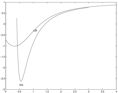
Figure 1: Comparison between Reisnner-Nordström (RN) and $\Psi(r)$ (LBI) [$\alpha=0.1$, $Q=1$, $\Lambda=0$, $b=1$, $m=\pi$].

Depending on the values of the parameters of the black hole (charge $Q$, mass $m$, Born-Infeld constant $b$ and Gauss-Bonnet constant $\alpha$) the square root could be imaginary. If $\alpha>0$ and $m\geq\frac{\pi}{2}\>b^{2}\>L^{4}\>\gamma=m_{c}\;\;$ the solution is valid for all $r\geq 0$.

If $m>m_{c}$ then $\Psi(0)\neq 1$, so the metric has a conical singularity at the origin: whereas the equator measures $2\>\pi\>r$, the radius at the equator is $\int_{o}^{r}\>\frac{dr}{\sqrt{\Psi(r)}}$. In the critical case $m=m_{c}$ one finds $\Psi(0)=1$ and the conical singularity disappears from the metric since in this case $\int_{o}^{r}\>\frac{dr}{\sqrt{\Psi(r)}}\approx r$ when $r\approx 0$.

Conversely, we can think in the critical value $m_{c}$ as follows: we can define a critical value $Q^{2}_{c}=b^{-1}\left(\frac{2m}{\pi\gamma}\right)^{3/2}$ which represents an upper bound on $Q$ for the metric (24) to be well defined in the whole spacetime. Thus, a critical value for the black hole charge appears in this context as a direct consequence of the finite-$b$ effects. The role payed by $b$ is setting the critical value $Q_{c}\to 0$ in the Maxwellian regime $b\to\infty$, which is consistent with the fact that the Lovelock-Maxwell black hole geometry is not regular if $m\neq 0$.

Besides, the finite-$b$ effects act in (22) as a kind of effective cosmological constant $\Lambda_{eff}(r)=\Lambda+2b^{2}(1-e^{u_{b}(r)})$, with $u_{0}=0$ and $\displaystyle\lim_{r\to\infty}u_{b}(r)=0$. Thus, this fact could lead one to infer that the dressing of the black hole parameters discussed in section II can also receive contribution due to the presence of $b$. However, this is not the case, as it can be verified by noting that no $b$-dependent quadratic terms in $r$ arise when expanding the right hand side of (22).

In this geometry, the position of the horizon $r_{h}$ is defined by $\Psi(r_{h})=0$, then

$$r_{h}^{2}=\frac{2\>m}{\pi}-2\>\alpha-\frac{r_{h}^{4}}{12}(4\>b^{2}-2\>\Lambda)+\frac{b^{2}}{3}\>r_{h}\>\sqrt{r_{h}^{6}+L^{6}}$$

$$-b^{2}\>L^{4}\>\int_{r_{h}/L}^{\infty}\>\frac{dt}{\sqrt{1+t^{6}}}$$

and thus, for $\Lambda=0$ and $m>m_{c}+\pi\>\alpha$ there is only one horizon. If $m\leq m_{c}+\pi\>\alpha$ then the solution is similar to Reissner-Nordström in the sense that there could be two horizons. When the equality holds one of the horizons is at the origin (see Eq. (25)). Figure 2 shows the position of the horizon ($r_{h}$) as a function of the mass $m$ for the Lovelock-Born-Infeld black hole and the Reissner-Nordström case ($b\rightarrow\infty$).

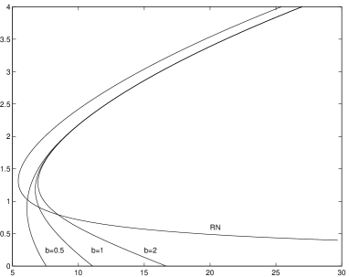
Figure 2: Event horizon position (vertical axis) as a function of the black hole mass (horizontal axis) for different values of $b$ and in the Reissner-Nordström case (RN) [$\alpha=0.5$, $Q=3$, $\Lambda=0$].

These graphics exhibit the crucial difference existing between the Lovelock-Born-Infeld black hole and the Reissner-Nordström black hole; namely the fact that for a given charge $Q$ there exists a finite value for the black hole mass $m$ such that the black hole geometry presents only one horizon, because the internal one reached the origin. This enhancement of the region bounded by both internal and external horizons is also $b$-dependent and represents, by itself, one of the principal distinctions between the black hole geometries in both theories. Moreover, Fig. 2 shows how the extremal configuration $r_{+}=r_{-}$, which is translated into a complicated expression in terms of the parameters $m,Q,\alpha$ and $b$, experiments a displacement for finite values of $b$ with respect to the Reissner-Nordström configuration $m^{2}=\frac{\pi^{2}}{3}Q^{2}$. Figure 3 shows different behaviors of the solution $\Psi(r)$ for different values of b. This parameter controls the cualitative behaviour close to the origin. The metric for the subcritical case ($m<m_{c}$) is not well defined in the whole spacetime.

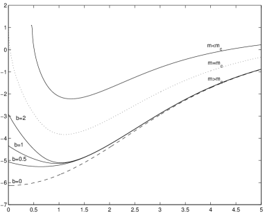
Figure 3: Graphics of $\Psi(r)$ for different values of $b$, for $m<m_{c}$: [$m=2$, $\alpha=0.5$, $Q=1$, $b=2$, $\Lambda=0$], for $m=m_{c}$ [$m=3.49$, $\alpha=0.5$, $Q=1$, $b=2$, $\Lambda=0$] and for $m>m_{c}$ [$m=5$, $\alpha=0.5$, $Q=1$, $\Lambda=0$].

V Thermodynamics

Now, let us move to the thermodynamics of the vacuum solution. The Hawking temperature of the black hole is proportional to the surface gravity $\kappa$ and it is given by the formula

$$T=\frac{\hbar}{4\pi k_{B}}\kappa$$ (26)

where $k_{B}$ is the Boltzmann constant. In order to calculate $\kappa$ we must evaluate the derivative of $g_{00}$ in the exterior horizon radius $r_{h}$. From the Lovelock vacuum solution (11) with $\Lambda=0$ we obtain $r_{h}=\sqrt{\frac{2\>m}{\pi}-2\alpha}$. Hence, the surface gravity of the corresponding geometry results

$$\kappa=\frac{\sqrt{\frac{2m}{\pi}-2\alpha}}{\alpha(1+\frac{m}{\pi\alpha})}=\frac{2\>r_{h}}{4\alpha+r_{h}^{2}}$$

and the Hawking temperature is given by

$$T=\frac{\hbar}{2\pi k_{B}}\frac{r_{h}}{4\alpha+r_{h}^{2}}$$ (27)

Notice that the temperature goes to zero for bigger black holes ($r_{h}\rightarrow\infty$). This behaviour is the same of the Schwarzschild black hole. A remarkable results is that, unlike the Schwarzschild case, for small black holes ($r_{h}\rightarrow 0$ or $m\rightarrow m_{c}$) the temperature also goes to zero and there would not be Hawking radiation (Fig. 4). On the other hand, when $\alpha\rightarrow 0$ in equation (27) we recover the general relativity result since, in that case, the temperature is proportional to the inverse of the radius.

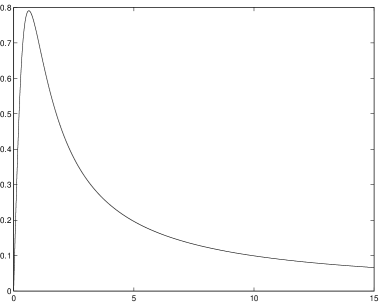
Figure 4: Hawking temperature as a function of the horizon radius [$\alpha=0.1$, $\Lambda=0$].

The specific heat $c$ is given by

$$c=\frac{\partial m}{\partial r_{h}}\Bigg{(}\frac{\partial T}{\partial r_{h}}\Bigg{)}^{-1}=\frac{2\pi^{2}k_{B}}{\hbar}\frac{r_{h}(4\alpha+r_{h}^{2})^{2}}{4\alpha-r_{h}^{2}}$$ (28)

and, from this, we observe that the position $r_{0}=\sqrt{4\alpha}$ $(m=3\pi\alpha)$, where the specific heat changes the sign (Fig. 5), represents a transition point (in the Fig. 4 this point is the maximum). When $r_{h}<r_{0}$ the specific heat is positive and the black hole is stable; while in the range $r_{h}>r_{0}$ the specific heat is negative and the black hole turns out to be, in this sense, unstable. The temperature of this transition point is $\displaystyle T_{0}=\frac{\hbar}{2\pi k_{B}}\frac{1}{\sqrt{4\alpha}}$.

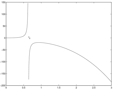
Figure 5: Black hole specific heat as a function of the horizon radius [$\alpha=0.1$, $\Lambda=0$].

Regarding the entropy of this black hole solution, we make use of the fact that the first law for this non-rotating black hole can be written as usual,

$$T\>\delta S=\delta m$$ (29)

where $\delta m=\pi\>r_{h}\>\delta r_{h}$. Thus the entropy results

$$S=\frac{\pi^{2}k_{B}}{2\hbar}(12\alpha\>r_{h}+r_{h}^{3})$$ (30)

In the limit $\alpha\rightarrow 0$ the entropy is proportional to the area of the event horizon, in agreement with the Bekenstein-Hawking formula. On the other hand, the first term in the equation (30) is a consequence of the Gauss-Bonnet term. It is possible to see that this correction term in the entropy formula is proportional to the integral of the scalar curvature invariant of the horizon wald (34). This computation confirms, by means of a concise example, the observation derived from Hamiltonian methods in mayer (35) about the fact that the entropy of Lovelock black holes is not simply the area formula, but topological invariants also contributes to the whole entropy. This aspect was also discussed in myers2 (25).

Besides, by using the Stefan-Boltzmann law in five dimensions to compute the flux of thermal radiation we can approximately obtain the black hole evaporation time $\Delta t$; namely

$$\frac{dm}{dt}=\pi r_{h}\frac{dr_{h}}{dt}\propto T^{5}r_{h}^{3}$$ (31)

With the expression for the Hawking temperature (27) and integrating (31) one finds that the lifetime of the Lovelock black holes turns out to be infinite. This is due to the linear dependence between the temperature and the horizon radius for small black holes. Hence, these are eternal black holes.

Furthermore, we find that the themodynamics of the Lovelock black holes in presence of a negative cosmological constant is also consistent with the known results of Einstein gravity solutions within the appropriate range. Certainly, the Lanczos Lagrangian represents short-distance corrections to Einstein gravity which start to be relevant at scales comparable with $l_{L}\sim\sqrt{\alpha}$, which we could denominate Lanczos-Lovelock scale. Conversely, the value of the cosmological constant $\Lambda$ introduces another length scale, given by $l_{\Lambda}\sim\Lambda^{-2}$, which marks the scales where the cosmological term starts to dominate. Hence, we can identify the range bounded by the maximum and the minimum of Fig. 6 as the scales where the results coming from general relativity fit the thermodynamic behaviour of the Lovelock solution. Consequently, for very large scales (large black holes) the thermodynamic behaviour is well approximated by the AdS-Schwarzschild black hole solution while the short distance corrections start to dominate at the scale $l_{L}$.

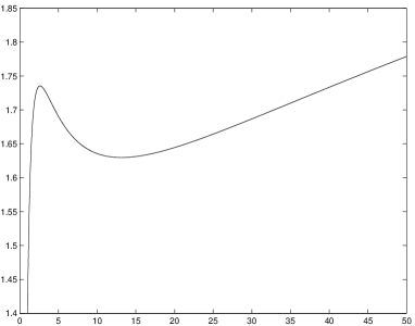
Figure 6: Hawking temperature for a negative cosmological constant as a function of the mass [$\alpha=0.1$, $\Lambda=-0.6$].

Within this context, we can also notice that the thermodynamical properties of the black hole geometry that appears in the case $\Lambda\alpha=-\frac{3}{4}$ (with $\Lambda<0$) exhibit particular features. Indeed, as we early mentioned, this case is analogous to the BTZ three-dimensional black hole since the phase diagram involving the temperature and the mass is a monotonic function (see Fig. 7) describing a phase such that the specific heat is positive everywhere. In some sense, this case can be considered as a transition and, thus, its stability could be an interesting point to be studied with particular attention. The temperature of these black holes is given by $T=\frac{\hbar}{2\pi k_{B}}\frac{r_{h}}{4\alpha}$; this goes to zero for large $\alpha$ and identically vanishes for the critical mass $m=\pi\alpha$.

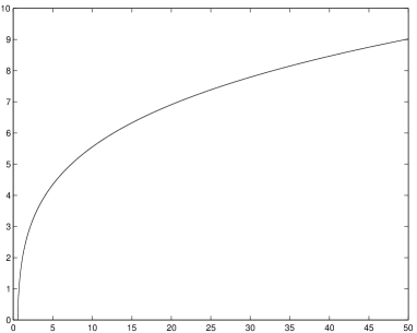
Figure 7: Hawking temperature for the case $\Lambda\alpha=-\frac{3}{4}$ as a function of the mass [$\alpha=0.1$, $\Lambda=-7.5$].

VI Conclusions

In this paper we studied a solution (22) representing five-dimensional charged black holes in Lovelock gravity coupled to Born-Infeld electrodynamics. The corrections induced by the quadratic terms in the Lagrangian (Gauss-Bonnet terms) correspond to short-distance modifications to general relativity and, therefore, the relevant differences between both theories appear for small radius.

The Lovelock-Born-Infeld black holes are characterized by the mass ($m$), the Gauss-Bonnet constant ($\alpha$), the charge ($Q$) and the Born-Infeld constant ($b$). The constant $\alpha$ must be positive in order to have a well behaved solution for all value of $r$. The metric does not diverge at $r=0$; for the critical mass $m=m_{c}$ the conical singularity, which is characteristic of the Hoffmann-Born-Infeld solution, is removed (nevertheless, the origin is a curvature singularity).

We commented the differences existing with respect to the Reissner-Nordström black holes and, from this analysis, we observed that, unlike the general relativity, the Lovelock-Born-Infeld theory admits charged black hole solutions with only one horizon. This is due to the fact that for a given charge $Q$, there exist values of mass that force the internal black hole radius to reach the origin.

There is another important distinction between the solutions of both theories. Also in contrast to the Schwarzschild solution, the temperature of the black hole remains finite; in particular, we showed that the temperature goes to zero when the horizon radius approximates to the origin, and there is not Hawking radiation. This leads to find an infinite lifetime for Lovelock solutions because the short-distance effects render the small black holes stable. The temperature of the transition point, where the short-distance corrections start to be relevant, is $T=\frac{\hbar}{\pi k_{B}}\frac{1}{\sqrt{4\alpha}}$, which corresponds to black holes with a size comparable to the Lovelock-Lanczos scale, $r=2l_{L}$.

We discussed different limits of the solutions in terms of the coupling constant of Lanczos Lagrangian $\alpha$ and Born-Infeld Lagrangian $b$, and we proved that these limits correspond to the expected geometries. Hence, the solution we present here represents a geometry interpolating between the quoted Hoffmann metric for Einstein-Born-Infeld theory and the solution found by Wiltshire for the case of Lovelock-Maxwell field theory. Furthermore, we showed how other solutions studied in the literature are included as particular cases, representing a BTZ phase which arises on the curve $\Lambda\alpha=-\frac{3}{4}$ in the space of parameters. We discussed the similar features of this phase and the Anti-de Sitter black holes.

- (1) Lovelock D., J. Math. Phys. 12, 498 (1971).
- (2) Bañados M., Teitelboim C. and Zanelli J., Lovelock-Born-Infeld Theory of Gravity in J.J. Giambiagi Festschrift, La Plata (edited by Falomir H., Gamboa R. RE., Leal P. and Schaposnik F., World Scientific, Singapore) (1990).
- (3) Fradkin E. S. and Tseytlin A. A., Phys. Lett. B 163, 12 (1985).
- (4) Bergeshoeff E., Sezgin E., Pope C. N. and Townsend P.K., Phys. Lett. B 188, 70 (1987).
- (5) Metsaev R.R., Rahmanov M. A. and Tseytlin A. A., Phys. Lett. B 193, 207 (1987).
- (6) Zwiebach B., Phys. Lett. B 156, 315 (1985).
- (7) Cai Y. and Nuñez C., Nucl. Phys. B 287, 279 (1987).
- (8) Gross D.J. and Sloan J.H., Nuc. Phys. B 291, 41 (1987).
- (9) Crisostomo J., del Campo S. and Saavedra J., Hamiltonian treatment of Collapsing Thin Shells in Lanczos-Lovelock’s theories [arXiv:hep-th/hep-th/0311259]
- (10) Rong-Gen Cai, Phys. Lett. B 582, 237, (2004). Rong-Gen Cai, Phys. Rev. D63, 124018 (2001).
- (11) Izaurrieta F., Rodríguez E. and Salgado P., Phys. Lett. B 586, 397, (2004). Navarro I. and Santiago J., JHEP 0404, 62 (2004). Rong-Gen Cai and Kwang-Sup Soh, Phys. Rev. D59, 044013 (1999). Lemos J.P., A Profusion of Black Holes from Two to Ten Dimensions, Proceedings of the XVIIth Brazilian Meeting of Particle Physics and Fields, (edited by Adilson J. da Silva et al) (1997). Allemandi G., Francaviglia M. and Raiteri M., Class. and Quant. Grav. 20, 5130 (2003). Ilha A., Kleber A. and Lemos J.P., J. Math. Phys. 40, 3509 (1999).
- (12) Hoffmann B., Phys. Rev. 47, 877 (1935).
- (13) Gibbons G. W. and Rasheed D. A., Nuc. Phys. B 454, 185 (1995).
- (14) D’Olivera H., Class. Quant. Grav. 11, 1469 (1994).
- (15) Deruelle N., Phys. Rev. D 41, 3696 (1990).
- (16) Misner C.W., Wheeler J.A. and Thorne K.S., Gravitation (Freeman, San Francisco) (1973).
- (17) Lanczos C., Z. Phys. 73, 147 (1932).
- (18) Lanczos C., Ann. Math. 39, 842 (1938).
- (19) Müller-Hoissen F., Phys. Lett. B 163 , 106 (1985).
- (20) Paterson E.M., J. London Math. Soc. 23(2), 349 (1981).
- (21) Lovelock D., Tensors, Differential Forms and Variational Principles (Wiley-Interscience, New York) (1975).
- (22) Wiltshire D., Phys.Rev.D 38 2445 (1988).
- (23) Louko J., Simon J.Z. and Winters-Hilt S.N., Phys.Rev. D 55, 3525 (1997).
- (24) Myers R.C. and Simon J.Z., Phys.Rev.D 38 2434 (1988).
- (25) Bañados M., Teiltelboim C. and Zanelli J., Phys. Rev. Lett 69, 13 (1992).
- (26) Bañados M., Henneaux M., Teiltelboim C. and Zanelli J., Phys. Rev. D 48, 1506 (1993). Horowitz G. and Welch D., Phys. Rev. Lett. 71, 328 (1993). Coussaert O., Henneaux M. and van Driel P., Class. Quant. Grav. 12, 2961 (1995). Coussaert O. and Henneaux M., Phys. Rev. Lett. 72, 183 (1994).
- (27) Bañados M., Black Holes in Einstein-Lovelock Gravity, Talk given at the VIII Latin American Symposium on Relativity and Gravitation, SILARG, Sao Paulo, July 1993, [arXiv:hep-th/9309011]. Bañados M., Teitelboim C. and Zanelli J., Phys. Rev. D49, 975 (1994). Crisostomo J., Troncoso R.and Zanelli J., Phys.Rev.D 62, 084013 (2000).
- (28) Born M. and Infeld L., Nature 132, 1004 (1933).
- (29) Born M. and Infeld L., Proc. Roy. Soc. (London) 144, 425 (1934).
- (30) Plebanski J., Lectures on non linear electrodynamics (Nordita Lecture Notes, Copenhagen) (1968).
- (31) Franklin P., Methods of Advanced Calculus (Mc. Graw Hill, London) (1944).
- (32) Wiltshire D. L., Phys. Lett. B 169, 36 (1986).
- (33) Wald R.M., Phys. Rev. D 48, R3427 (1993).
- (34) Jacobson T. and Myers R.C., Phys. Rev. Lett. 70, 3684 (1993).