Late time tails from momentarily stationary, compact initial data in Schwarzschild spacetimes

Abstract

Abstract

An $\ell$-pole perturbation in Schwarzschild spacetime generally falls off at late times $t$ as $t^{-2\ell-3}$. It has recently been pointed out by Karkowski, Świerczyński and Malec, that for initial data that is of compact support, and is initially momentarily static, the late-time behavior is different, going as $t^{-2\ell-4}$. By considering the Laplace transforms of the fields, we show here why the momentarily stationary case is exceptional. We also explain, using a time-domain description, the special features of the time development in this exceptional case.

I Introduction

The perturbations in Schwarzschild spacetime radiate into the horizon and out to future null infinity (Scri+), so that at any fixed position in Schwarzschild coordinates, the perturbation falls off in time $t$. It has long been known that the fall-off is an inverse power-law in time of the form $t^{-n}$. For a multipole perturbation of multipole index $\ell$, the value of the power law index $n$ can take several forms. In the case of a perturbation that, at large radius, has the asymptotic form of a static multipole, $n=2\ell+2$. This case is of particular astrophysical interest since it describes the fate of initial multipoles coupled to a star that has been stationary, but undergoes gravitational collapse to a black hole price . This result has been confirmed, for example, by Cunningham, Price, and Moncrief cpm , and more recently by Baumgarte and Shapiro, in the context of the collapse of magnetized neutron stars baumshap .

In the case of an initial moment that is asymptotically static, the initial field at large radius is the limiting factor in the rate at which the field falls off. The fall-off is faster if the initial data has compact support. The rule in this case is $n=2\ell+3$ price ; manyrefs ; barack . This result was found numerically also for fully-nonlinear spherical collapse of a scalar field gpp ; bo . Recently, however, Karkowski, Świerczyński and Malec karkswiermalec , hereafter KSM, presented numerical evidence that if the data are momentarily stationary as well as being of compact support, then $n=2\ell+4$. Here we will explain, from two different points of view, why the momentarily static case is an exception.

Perturbations of spherically symmetric black holes can be decomposed into multipoles, and each multipole moment $\Psi(x,t)$ satisfies an equation of the form

$$\frac{\partial^{2}\Psi}{\partial x^{2}}-\frac{\partial^{2}\Psi}{\partial t^{2}}-V(x)\Psi=0\,.$$ (1)

In the specific case of perturbations of a Schwarzschild spacetime of mass $M$, the variable $t$ is the usual Schwarzschild time coordinate and $x$ is the ‘tortoise’ coordinate, related to the Schwarzschild radial coordinate $r$ by $x\equiv r_{*}=r+2M\ln{(r/2M-1)}$. Here we use units in which $G=1=c$; we choose $M=1$ without loss of generality, so that $t$ and $x$ are dimensionless. If $\Psi$ represents odd-parity gravitational perturbations, then the potential $V(x)$ is the Regge-Wheeler RW potential; if $\Psi$ represents even-parity gravitational perturbations, $V(x)$ is the Zerilli zerilli potential. For even- or odd-parity electromagnetic perturbations, or for scalar perturbations, $V(x)$ has a somewhat different form. It will be convenient here for us not to specify at the outset just what particular form $V(x)$ takes. We will require only that $V(x)$ falls off sharply as $x\rightarrow-\infty$  and that $V(x)=\ell(\ell+1)x^{-2}\{1+{\cal O}[\ln(x)/x]\}$, for large $x$.

In the next section we work with the Laplace transform of $\Psi(x,t)$, and relate the Laplace transform to an integral over the initial data. In principle, the form of the late-time tails of the perturbations can be extracted from the analytic details of Green functions in Laplace or Fourier space, as others have shown leaver ; laplace . Indeed, as shown by Leaver leaver , the late time tails will be a sum of a $t^{-2\ell-3}$ tail and a $t^{-2\ell-4}$ tail, the latter term arising from time-symmetric initial data. But we can avoid such complications. If one accepts that $n=2\ell+3$ is the result for generic initial data of compact support, it turns out that an immediate consequence is that $n$ must be $2\ell+4$ if the initial data are momentarily stationary.

The late-time tails are usually thought of as a result of backscatter of radiation by the potential $V(x)$ at large radius. Though the proof in Sec. II is definitive, it does not explain how, in the scattering picture, the momentarily stationary initial data are exceptional. In Sec. III we provide a heuristic explanation by showing that for the momentarily stationary case, the initial data result in two outgoing pulses that, in a sense, cancel each other.

The exceptional behavior of time-symmetric initial data can suggest the following paradox: Take the effective potential to be that of a Schwarzschild spacetime, but truncate it below a certain value of the Regge-Wheeler ‘tortoise’ coordinate $r_{*}$, and take this truncation to be at a large negative value of $r_{*}$. For the generation of tails, such a truncated potential is expected to be an excellent approximation to the full Schwarzschild potential, because the Schwarzschild potential drops off exponentially with $r_{*}$ for large and negative values of $r_{*}$, and as is well known, it is only the form of the effective potential at large distances (large and positive values of $r_{*}$) that is important for the tails problem in Schwarzschild. Consider first initial data of an outgoing pulse of compact support to the “left” (more negative $r_{*}$ side) of the truncated potential, so that the initial pulse is fully located in the region of zero potential. One could expect the tail in this case to be given by $t^{-2\ell-3}$, since the initial outgoing pulse is generic time-asymmetric initial data. Consider next the same situation, but this time with an initially momentarily static pulse of twice the amplitude of the initially outgoing pulse we previously considered. The compact initial pulse is in a region of spacetime with zero potential, and therefore will immediately split into outgoing and incoming pulses. The latter is never heard from again; it travels to the left in a region of zero potential, and therefore never scatters. The pulse traveling to the right is identical to the situation we considered above. However, in this case, based on the prediction of KSM, the tails should be given by $t^{-2\ell-4}$. How can we explain this paradox, and what is the correct form of the tail in this situation? We conclude this paper by resolving this conflict of predictions.

II Relation of tails to initial data

We now follow the approach used by several authors leaver ; laplace , and introduce the Laplace transform $\psi(x,s)$ of $\Psi(x,t)$ through

$${\cal L}[\Psi(x,t)]\equiv\psi(x,s)=\int_{0}^{\infty}e^{-st}\Psi(x,t)\,dt$$ (2)

and the inverse

$${\cal L}^{-1}[\psi(x,s)]\equiv\Psi(x,t)=\frac{1}{2\pi i}\int_{\Gamma}e^{st}\psi(x,s)\,ds\,,$$ (3)

where $\Gamma$ is a vertical contour in the right half of the complex $s$ plane. With the relation ${\cal L}(\partial\Psi/\partial t)=-\Psi(x,t=0)+s\psi(x,s)$, and its extension to second time derivatives, we write the Laplace transform of Eq. (1) as

$$\frac{\partial^{2}\psi}{\partial x^{2}}-\left[s^{2}+V(x)\right]\psi=S(x,s)=-s\Psi_{0}(x)-\dot{\Psi}_{0}(x)\,.$$ (4)

Here $\Psi_{0}$ and $\dot{\Psi}_{0}$ are, respectively, the initial ($t=0$) value of $\Psi(x,t)$ and the initial value of $\partial\Psi(x,t)/\partial t$.

To solve Eq. (4), we again follow the approach of several authors leaver ; laplace ; we define homogeneous solutions $y_{L}(x,s)$ and $y_{R}(x,s)$ of Eq. (4) that, respectively, represent waves moving inward through the horizon, and outward at spatial infinity:

$$y_{L}\stackrel{{\scriptstyle x\rightarrow-\infty}}{{\sim}}e^{sx}\quad\quad\quad y_{R}\stackrel{{\scriptstyle x\rightarrow+\infty}}{{\sim}}e^{-sx}\,.$$ (5)

The Green function can be constructed in the usual way from $y_{L}$ and $y_{R}$, and the solution to Eq. (4) is given by

$$\psi(x,s)=\frac{1}{W(s)}\left[y_{R}(x,s)\int_{-\infty}^{x}y_{L}(x^{\prime},s)S(x^{\prime},s)\,dx^{\prime}+y_{L}(x,s)\int_{x}^{\infty}y_{R}(x^{\prime},s)S(x^{\prime},s)\,dx^{\prime}\right]\,,$$ (6)

$W(s)$ being the Wronskian determinant of the homogeneous solutions. We next use the form of $S(x,s)$ in Eq. (4) to write Eq. (6) as

$$\psi(x,s)=\psi_{0}(x,s)+\dot{\psi}_{0}(x,s)\,,$$ (7)

where

$$\psi_{0}(x,s) = \frac{-s}{W(s)}\left[y_{R}(x,s)\int_{-\infty}^{x}y_{L}(x^{\prime},s)\Psi_{0}(x^{\prime})\,dx^{\prime}+y_{L}(x,s)\int_{x}^{\infty}y_{R}(x^{\prime},s)\Psi_{0}(x^{\prime})\,dx^{\prime}\right]$$ (8)

$$\dot{\psi}_{0}(x,s) = \frac{-1}{W(s)}\left[y_{R}(x,s)\int_{-\infty}^{x}y_{L}(x^{\prime},s)\dot{\Psi}_{0}(x^{\prime})\,dx^{\prime}+y_{L}(x,s)\int_{x}^{\infty}y_{R}(x^{\prime},s)\dot{\Psi}_{0}(x^{\prime})\,dx^{\prime}\right]\,.$$ (9)

Now let us suppose that $\dot{\Psi}_{0}(x)$ and ${\Psi}_{0}(x)$ are arbitrary (bounded) functions of compact support, and for every choice of these functions, except perhaps the choice $\dot{\Psi}_{0}(x)=0$, let us suppose that the fields at any value of $x$ fall off as $t^{-2\ell-3}$. From this we conclude that for any bounded $f(x)$ of compact support the expression

$$F(x,s)=\frac{-1}{W(s)}\left[y_{R}(x,s)\int_{-\infty}^{x}y_{L}(x^{\prime},s)f(x^{\prime})\,dx^{\prime}+y_{L}(x,s)\int_{x}^{\infty}y_{R}(x^{\prime},s)f(x^{\prime})\,dx^{\prime}\right]\,,$$ (10)

gives the Laplace transform of a function that falls off in time no slower than $t^{-2\ell-3}$. Now note that $sF(x,s)$ is the Laplace transform of the time derivative of this function, and that the time derivative will fall off as $t^{-2\ell-4}$. We can therefore conclude that if the generic late time behavior is $t^{-2\ell-3}$, then $\dot{\psi}_{0}(x,s)$ is the transform of a function that falls off as $t^{-2\ell-3}$ and ${\psi}_{0}(x,s)$ is the transform of a function that falls off as $t^{-2\ell-4}$. In the exceptional case that the initial data is momentarily stationary, $\dot{\psi}_{0}(x,s)$ vanishes, and the late time behavior is $t^{-2\ell-4}$.

III The backscatter of momentarily stationary compact initial data

To explain the $n=2\ell+4$ tails we shall use the general heuristic framework developed in Refs. ori ; barack : consider that there is a background problem, with a zero-order potential

$$V_{0}^{\ell}\equiv\left\{\begin{array}[]{cl}\ell(\ell+1)/x^{2}&x>x_{0}\\ 0&x<x_{0}\end{array}\right.\,.$$ (11)

We will consider the remainder of the potential to be a perturbation, so that $V(x)=V_{0}^{\ell}+\epsilon\,\delta V$. The $\epsilon$ is an accounting device so that we carry out a sort of perturbative analysis.

The idea of this division of the potential into a background part and a perturbation is that the background is a pure centrifugal potential that cannot produce long-lived radiative tails. The tails, therefore, must be due to $\delta V$. The (scalar field) monopole case is somewhat awkward, since the centrifugal potential vanishes. What we really need though is some “edge” at some $x_{0}$. Barack barack discusses the possibility of using a delta function for this purpose, but we need not be specific. Despite its awkward feature, we shall rely heavily on the monopole case. This is not solely because the slowly decaying $\ell=0$ tails are the easiest to compute to long times. More important, the description of backscatter for the $\ell=0$ case, lacks technical complications of higher order multipoles. To focus on the essential ideas of backscatter, we shall therefore confine ourselves to $\ell=0$. The extension to higher $\ell$ is straightforward.

We shall confine ourselves to descriptions to first order in $\epsilon$. This, sensu stricto, is not correct but we believe that the fundamental picture that comes out of that first-order analysis is correct. Strong evidence for this is the numerical accuracy (illustrated below in Fig. 3) of a prediction coming from this picture.

As in Ref. barack , we shall introduce advanced time $v$ and retarded time $u$ by

$$v=t+x\quad\quad u=t-x\,,$$ (12)

and we shall focus attention, not on tails at ${\cal I}^{+}$ (that is, $t\rightarrow\infty$ at constant $x$), but rather at Scri+ (that is, $v\rightarrow\infty$ at constant $u$). It can be shown price ; barack that the tails at Scri+ and at ${\cal I}^{+}$ are tightly connected. If the former is $u^{-m}$ then the latter is $t^{-m-\ell-1}$. For the monopole case, then, we need to show that for generic initial data of compact support, the tail at Scri+ falls off as $u^{-2}$, while for momentarily stationary initial data of compact support the tail has the form $u^{-3}$.

To simplify some statements in our analysis, we will not deal with the monopole potential per se, but rather, shall take our potential to be strictly zero for $x<x_{0}$, and to be $1/x^{3}$ for $x>x_{0}$. We now write Eq. (1), to first order in $\epsilon$ as

$$\Psi_{(1),uv}=-\frac{1}{4}\,\epsilon\;\delta V\Psi_{0}\,.$$ (13)

Let us suppose that the zeroth order solution is an outgoing pulse $\Psi=F(u)$ of compact support. Following the steps in Ref. barack , and making the same approximations, we get

$$\Psi_{(1)}=-\epsilon\,\frac{1}{4}\int_{-\infty}^{u}F(u^{\prime})\,du^{\prime}\int_{u+2x_{0}}^{\infty}dv^{\prime}\,\delta V(x^{\prime})\,.$$ (14)

When we use our special form of the potential $\delta V=1/x^{3}$, this becomes

$$\Psi_{(1)}=-\epsilon\,\frac{1}{4}\int_{-\infty}^{u}F(u^{\prime})du^{\prime}\,\int_{u+2x_{0}}^{\infty}dv^{\prime}\,\frac{8}{(v^{\prime}-u^{\prime})^{3}}\approx-\frac{\epsilon}{u^{2}}\int_{-\infty}^{\infty}F(u^{\prime})du^{\prime}\,.$$ (15)

We have used the same approximations here as those of Ref. barack . In particular, we have assumed that the value of $u$ to which this tail result is to be valid satisfies $u\gg u^{\prime}$, where $u^{\prime}$ is any point in the support for $F$ accuracy .

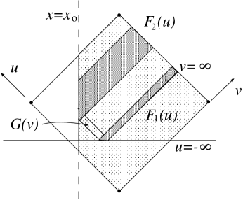
Figure 1: The evolution of momentarily stationary initial data of compact support. The figure shows the zeroth order pulses $F_{1}(u)$, $G(v)$, and $F_{2}(u)$ described in the text.

We now consider the case of initial data that are momentarily stationary. The zero-order solutions for such initial data will immediately “split” into an ingoing pulse and an outgoing pulse. These are labeled as $F_{1}(u)$ and $G(v)$ in Fig. 1. (Note that $v$ has been conformally rescaled in the figure to bring Scri+ to a finite location.) In the special case of momentarily stationary initial data the ingoing and outgoing zero-order pulses will be related by $G(\xi)=F_{1}(-\xi)$. The “edge” at $x=x_{0}$ is a zero-order feature, so the ingoing $G(v)$ will undergo partial reflection at $x_{0}$ and will generate a second outgoing pulse $F_{2}(u)$.

For there to be no $u^{-2}$ tail at Scri+ (and hence no $t^{-3}$ tail at ${\cal I}^{+}$) it must be the case that $\int_{-\infty}^{+\infty}\left[F_{1}(u)+F_{2}(u)\right]\,du=0$. We have numerically checked a large number of examples, with different potentials, and different momentarily stationary initial data. In all cases we have found that the “cross section” (i.e. , the $u$ integral) of the reflected pulse $F_{2}(u)$ is opposite in sign to $F_{1}(u)$ and to numerical accuracy is equal in magnitude. Since $G(\xi)=F_{1}(-\xi)$, this is equivalent to

$$\int G(v)\,dv+\int F_{2}(u)\,du=0\,.$$ (16)

In practice, we integrated at $t={\rm const}$ over the outgoing part of the field. To have a numerically zero integral, the reflected field $F_{2}$ must have the opposite sign to the initial field $F_{1}$. In Fig. 2 we show the field at different values of the time as a function of the ‘tortoise’ coordinate. The figure shows the field soon after the time-symmetric initial data split into outgoing and incoming fields. As the outgoing field arrives at the peak of the effective potential the field scatters, and part is reflected toward the left with the opposite sign (and never heard from again), and a field of the opposite sign continues to move toward the right, following the main pulse. That is, the outgoing field is composed of the prompt field, and a broadened field of the opposite sign. It is the integral of the combined outgoing field that we calculate, and the result is shown in Fig. 3. In practice, we compute the integral only for positive values of $r_{*}$, to capture only the contributions from the outgoing field. However, at and near $r_{*}=0$ there is no clear separation between outgoing and incoming fields, and the field there is not strictly zero for finite values of time. Because of the contributions from the neighborhood of the peak of the effective potential, the integral does not vanish at finite values of time. However, the “area” between the field and the horizonal axis drops with time, and as $t\to\infty$ the integral approaches zero, like $t^{-2}$.

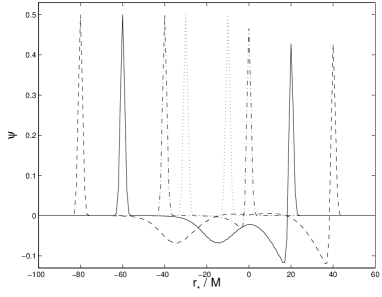
Figure 2: The field at four different value of the time. The initial data is that of a time-symmetric field centers at $r_{*}=-20M$, and the field is shown for $t=10M$ (dotted), $t=20M$ (dash-dotted), $t=40M$ (solid), and $t=60M$ (dashed curve).

area_time1.eps

Figure 3: The “area” integral of the outgoing field vs. the time. The circles represent the numerically integrated area, and the solid reference line is $7.44/t^{2}$. The errors in the numerical data are smaller than $1\%$.

This should not be misinterpreted as total reflection of the ingoing pulse $G(v)$, in the sense of total reflection of energy in the waves. Such a statement about reflection refers to a quantity quadratic in the wave pulse; the “reflected” pulse $F_{2}(u)$ is generally quite different in shape from the ingoing pulse $G(v)$, so Eq. (16) is very different from a claim of total energy reflection.

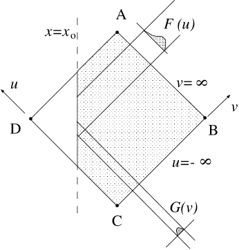
Figure 4: Reflection of an ingoing zeroth-order wave at the edge of the potential.

The relationship in Eq. (16) can be said to be the explanation for initially stationary initial data being a special case, and therefore of some importance. Though numerical verification of this relationship is its ultimate justification, it is interesting that there is a heuristic argument for Eq. (16) that helps us to understand it. Figure 4 shows a zeroth-order ingoing wave reflecting off the edge at $x=x_{0}$. For this situation, let us integrate the relationship in Eq. (13) over the range of $u,v$ shown in Fig. 4 as the rhombus with vertices $A$,$B$,$C$,$D$. The right hand side is clearly of order $\epsilon$. We make this explicit by writing

$$\int\int\Psi_{(1),uv}\,du\,dv=-\frac{1}{4}\epsilon\,\int\int\delta V\Psi_{(0)}\,du\,dv\,.$$ (17)

The integral on the left can immediately be evaluated:

$$\int\int\Psi_{(1),uv}\,du\,dv=\Psi_{(1)A}+\Psi_{(1)C}-\Psi_{(1)B}-\Psi_{(1)D}.$$ (18)

From causality we have

$$\Psi_{(1)C}=\Psi_{(1)D}=0\,.$$ (19)

By taking point $A$ at sufficiently large $u$, we can make $=\Psi_{(1)A}$ arbitrarily small. Point $B$ is is at $I^{+}$. The scattering of the ingoing pulse to $I^{+}$ is zero, so $\Psi_{(1)B}=0$.

We conclude that the left hand side of Eq. (17) vanishes, and this means that the integral on the right of Eq. (17) must vanish. We can break the right hand side integral into the contributions due to the zeroth order ingoing pulse $G(v)$ and the zeroth order outgoing pulse $F(u)$. For the ingoing pulse

$$\int\int\delta VG(v)\;du\,dv=2\int\int\delta VG(v)\;dx\,dv=2\int_{r_{0}}^{\infty}\delta V(x)\,dx\;\int G(v)\,dv\,.$$ (20)

If we add the outgoing contribution, we find that

$$2\int_{x_{0}}^{\infty}\delta V(x)\,dx\;\left[\int G(v)\,dv+\int F(u)\,du\;\right]$$ (21)

must vanish, and hence we have given a heuristic explanation for Eq. (16).

We are now in a position to revisit the paradox we described in the Introduction. There is a fundamental, although subtle, difference between the case of the truncated potential and the true Schwarzschild potential: In the latter case there is a small overlap of the initial data and the rapidly decreasing effective potential. Because of this overlap, there is no exact equivalence between outgoing initial data and time-symmetric initial data of twice the amplitude. Because the overlap is small, we expect the field from an initially outgoing pulse to fall off as $t^{-2\ell-4}$ at intermediate times. However, the small overlap implies that the true late time behavior will be $t^{-2\ell-3}$. This situation is demonstrated in Fig. 5, which shows the results for an initially outgoing field that is located to the left of the peak of the effective potential, for a spherically symmetric scalar field. At intermediate times the field clearly falls off like $t^{-4}$, but the asymptotic fall off is $t^{-3}$, as expected.

pulse_left.eps

Figure 5: A spherical scalar field in Schwarzschild. The initial data are for an outgoing compact pulse centered at $r_{*}/M=-40$. The solid line is the field, the dashed reference line is proportional to $t^{-4}$, and the dotted reference line is proportional to $t^{-3}$.

References

- (1) R.H. Price, Phys. Rev. D 5, 2419 (1972).
- (2) C.T. Cunningham, R.H. Price, and V. Moncrief, Astrophys. J. 224, 643 (1978); 230, 870 (1979).
- (3) T.W. Baumgarte and S.L. Shapiro, Astrophys. J. 585, 930 (2003).
- (4) C. Gundlach, R.H. Price, and J. Pullin, Phys. Rev. D 49, 883 (1994).
- (5) L. Barack, Phys. Rev. D 59, 044017 (1999).
- (6) C. Gundlach, R.H. Price, and J. Pullin, Phys. Rev. D 49, 890 (1994).
- (7) L.M. Burko and A. Ori, Phys. Rev. D 56, 7820 (1997).
- (8) J. Karkowski, Z. Świerczyński and E. Malec, Class. Quantum Grav. 21, 1303-1310 (2004).
- (9) T. Regge and J.A. Wheeler, Phys. Rev. 108, 1063 (1957).
- (10) F. Zerilli, Phys. Rev. D 2, 2141 (1970).
- (11) E.W. Leaver, Phys. Rev. D 34, 384 (1986).
- (12) Y. Sun and R.H. Price, Phys. Rev. D 38, 1040 (1988); H.-P. Nollert and B.G. Schmidt, Phys. Rev. D 45, 2617 (1992).
- (13) A. Ori, Gen. Relativ. Gravitation 29, 881 (1997).
- (14) Numerical experiments have confirmed that the amplitude of the tail at Scri+ is proportional to the integral of the outgoing pulse, but the numerical values found are smaller than those in Eq. (15) by a factor of around 0.88. This may be due to the contributions of higher order scattering.