The Penrose inequality and apparent horizons

Abstract

A spherically symmetric spacetime is presented with an initial data set that is asymptotically flat, satisfies the dominant energy condition, and such that on this initial data $M<\sqrt{A/16\pi}$, where $M$ is the total (ADM) mass and $A$ is the area of the apparent horizon. This provides a counterexample to a commonly stated version of the Penrose inequality, though it does not contradict the “true” Penrose inequality.

1 Introduction

For over 30 years, the Penrose inequality has been a major open question in classical general relativity, closely tied to an even bigger open question, the cosmic censorship conjecture. In 1973 Penrose [1] discussed attempts to find violations of the cosmic censorship conjecture. These attempts led him to formulate a certain inequality, the derivation of which relies so heavily on cosmic censorship that a violation of this inequality would go a long way towards contradicting it. Likewise, a proof of this inequality would strengthen the common belief in the validity of the cosmic censorship conjecture, though by itself a proof of the inequality would, of course, not serve as an actual proof of the conjecture.

Penrose’s original scenario was of a collapsing shell of null dust. A slightly modified presentation was given by Jang and Wald [2] who discussed this in the context of Cauchy initial data, i.e. a 3-manifold with a (complete) Riemannian metric, a symmetric tensor field representing the extrinsic curvature, and matter density and current. Repeating their discussion, the argument goes as follows: consider asymptotically flat initial data with Arnowitt–Deser–Misner (ADM) mass $M$ and an event horizon of area $A_{E}$. If cosmic censorship holds, this spacetime is expected to settle, eventually, to a Kerr–Newman black hole solution. Let $M_{K}$ be its mass and $A_{K}$ be the area of its event horizon. For the Kerr solution $M_{K}\geq\sqrt{A_{K}/16\pi}$. By Hawking’s area theorem [3], which assumes cosmic censorship, the area of the event horizon is non-decreasing, hence $A_{E}\leq A_{K}$. Furthermore the Bondi–Sachs energy radiated to null infinity is positive, so that the mass is non-increasing, $M\geq M_{K}$. It follows that for the initial data, $M$ and $A_{E}$ should satisfy

$$M\,\geq\,M_{K}\,\geq\,\sqrt{A_{K}/16\pi}\,\geq\,\sqrt{A_{E}/16\pi}$$ (1)

Assuming cosmic censorship and reasonable energy conditions the apparent horizon lies within the event horizon [4]. This leads to:

The Penrose inequality: Given any asymptotically flat initial data satisfying the dominant energy condition then

$$M\,\geq\,\sqrt{\mathcal{A}/16\pi}$$ (2)

with $M$ the total mass and $\mathcal{A}$ the minimum area required to enclose the apparent horizon.

Notice this rather delicate statement: though the apparent horizon lies inside the region enclosed by the event horizon, it need not be true that the area of the apparent horizon is smaller than the area of the event horizon. However, $\mathcal{A}\leq A_{E}$ still holds, hence the form that the Penrose inequality takes.

In recent years there has been much progress in proving the Penrose inequality in certain cases, though the general case is still open. Of note are proofs of the Riemannian Penrose inequality—the Penrose inequality in the time symmetric case. In this case the initial data has vanishing extrinsic curvature everywhere.  The requirement that the dominant energy condition be satisfied implies, in the time symmetric case, that the scalar curvature of this 3-manifold is everywhere non-negative.  Furthermore, the vanishing of the extrinsic curvature implies that the apparent horizon is an outermost minimal surface [5]. Hence in this case, $\mathcal{A}$ is equal to $A$, the area of the apparent horizon. Thus, the Riemannian Penrose inequality [5] is defined to be:

The Riemannian Penrose inequality: Given any asymptotically flat initial data satisfying the dominant energy condition, if, in addition, the extrinsic curvature vanishes, then

$$M\,\geq\,\sqrt{A/16\pi}$$ (3)

with $M$ the total mass and $A$ the area of the apparent horizon.

As mentioned, this has been proven by Huisken and Ilmanen [6], in the case where the apparent horizon is connected, thereby making rigorous the argument of [2] based on an original idea of Geroch [7]. More recently, Bray [8] proved this in a more general case, when the apparent horizon may consist of several disconnected components.

The form of the Riemannian Penrose inequality suggests a possible generalization:

The apparent horizon Penrose inequality: Given any asymptotically flat initial data satisfying the dominant energy condition, then

$$M\,\geq\,\sqrt{A/16\pi}$$ (4)

with $M$ the total mass and $A$ the area of the apparent horizon. (This is simply a modification of the Riemannian Penrose inequality by relaxing the requirement of time symmetry.)

The time symmetric case is a special one, as there, as mentioned above, one can replace the minimum area required to enclose the apparent horizon with the area of the apparent horizon itself. Thus Penrose’s original reasoning still applies to that case. But without the extra assumption of time symmetry, there does not seem to be any physical reason to expect the apparent horizon Penrose inequality to hold in general. Nevertheless there have been numerous appearances of this conjecture in the literature (e.g. [9, 10, 11, 12, 13]). With regard to the apparent horizon Penrose inequality, Bray and Chrusciel [5] state that a counterexample would not be terribly surprising, although it would be very interesting.

The main purpose of the present work is to provide an explicit counterexample to the apparent horizon Penrose inequality.

The remainder of the paper is organized as follows: Section 2 covers the required background on outer/inner trapped surfaces, especially in the Schwarzschild and Robertson–Walker (RW) spacetimes. In Section 3 spacetimes very much like (and including) the Oppenheimer–Snyder (OS) collapse model are described. These are used in Section 4 to obtain a counterexample to the apparent horizon Penrose inequality. A relevant issue pertaining to certain quasi-local constructions is discussed in Section 5. The paper concludes with a discussion of various versions of the inequality in an attempt to clarify what has been proven and which versions still stand a chance of holding.

The notation and conventions follow Wald [4].

2 Trapped surfaces

In order to make precise the inequality in question, the notion of outer/inner trapped surfaces is required.

Given a closed spacelike 2-surface, at each point there are precisely two future-directed null rays normal to the surface at that point. If the spacetime is asymptotically flat and the 2-surface is the boundary of a region that does not extend to the asymptotically flat end, one can distinguish between outgoing (towards the asymptotically flat region) and ingoing null rays. This motivates the next definitions, closely following Wald [4].

On a Cauchy surface, an outer (resp. inner) trapped surface is a compact smooth spacelike 2-manifold, which is the boundary of a region that does not extend to the asymptotically flat end, such that the expansion of outgoing (resp. ingoing) future-directed null geodesics normal to it is everywhere negative. A surface which is both outer trapped and inner trapped is a trapped surface.  A marginally outer (resp. inner) trapped surface is one where the above requirements are weakened so as to demand that the expansion of outgoing (resp. ingoing) null geodesics be only non-positive. On a Cauchy surface a trapped region is a region that does not extend to the asymptotically flat end and whose boundary is a marginally outer trapped surface. Finally, the total trapped region on a Cauchy surface is the closure of the union of all trapped regions in the Cauchy surface.

A trapped surface is an indication of a strong gravitational field. When the gravitational field is not so strong, one normally expects that the ingoing null rays will be converging while the outgoing ones will be diverging. Hence, for example, in Minkowski spacetime every 2-sphere with fixed $r$ and $t$ (in spherical coordinates) is inner trapped but the expansion of outgoing null geodesics in this case is everywhere positive (i.e. they diverge). In the other extreme, 2-spheres inside a Schwarzschild black hole region are trapped.

Given initial data, one can search the initial data 3-manifold for trapped surfaces. The notion of apparent horizon is extremely useful in this context, as the apparent horizon is defined to be the boundary of the total trapped region in the initial data 3-manifold. As a result the apparent horizon is marginally outer trapped with the expansion of future-directed, outgoing, null geodesics normal to it everywhere vanishing. Spherically symmetric initial data implies that the total trapped region is also spherically symmetric and therefore the apparent horizon is spherically symmetric as well.

It is known that in an asymptotically predictable spacetime satisfying the null energy condition, any marginally outer trapped surface (specifically, the apparent horizon) lies inside a black hole. Hence apparent horizons, which are local and therefore relatively easy to locate, are indicative of black holes. In general the black hole’s event horizon does not coincide with the apparent horizon. But being global, the event horizon requires a full knowledge of the spacetime’s causal structure before the event horizon’s actual existence is known, not to mention its exact location. Hence, for various applications, apparent horizons are more immediately accessible and practical.

With these definitions it is worthwhile to explore two specific spacetimes for the location of trapped surfaces. The discussion will prove useful, not only as concrete examples of the definitions above, but more importantly since these spacetimes will be ingredients in later constructions.

2.1 Maximally extended Schwarzschild spacetime

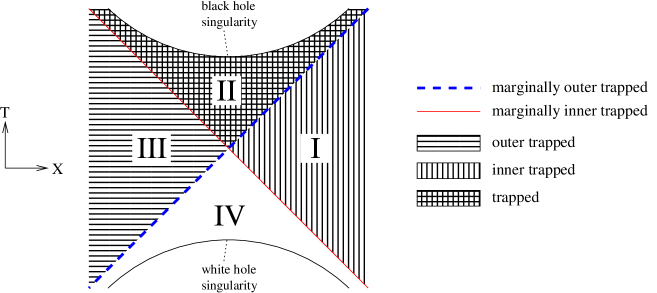
Figure 1: A spacetime diagram of the Kruskal extension of a Schwarzschild spacetime. Two angular dimensions are suppressed. Each point therefore represents a 2-sphere.

A spacetime diagram of the Kruskal extension of the Schwarzschild spacetime is shown in Fig. 1. In this case there are two asymptotically flat regions (Regions I and III), hence a designation of one of these regions as representing “infinity” is required in order to discuss outer and inner trapped surfaces. From now on, Region I is taken to contain infinity. The event horizon with respect to this choice of infinity is the surface (in the figure, a curve) separating Region I from II and separating Region III from IV. (From the perspective of the other asymptotically flat region, i.e. taking Region III to contain infinity, the figure is reversed (left to right) and so the event horizon in that case would be the surface separating Region II from III, and I from IV.)  The 2-spheres in Regions II and III are outer trapped. The 2-spheres in Regions I and II are inner trapped. Hence Region II consists of trapped 2-spheres. Region IV consists of 2-spheres that are neither inner nor outer trapped (it represents the white hole region and the 2-spheres in it would be outer and inner trapped if in the definitions above, future-directed null geodesics were replaced by past-directed ones). On any spherically symmetric Cauchy surface, the apparent horizon coincides with the event horizon. On it, the expansion of the outgoing null geodesics vanishes and the expansion of the ingoing ones is negative after the moment of time symmetry (in the portion separating Regions I and II) and is positive before that (in the portion separating Regions III and IV). The change in sign of the expansion of ingoing null geodesics is related to the difference between the white hole and black hole regions. This will be crucial to the construction of the counterexample.

2.2 Closed, dust-filled Robertson–Walker spacetime

A closed RW spacetime is a homogeneous, isotropic spacetime that starts from a singularity (the big bang) and ends in another (the big crunch). It has the line element

$$ds^{2}=-d\tau^{2}+a^{2}(\tau)\Big{(}d\chi^{2}+\sin^{2}\chi d\Omega^{2}\Big{)}$$ (5)

with $\chi\in[0,\pi]$. In the case of pressureless matter (dust) it is useful to introduce a parameter $\eta$ in terms of which the scale factor $a$ and proper time $\tau$ take the following forms [14]:

$$a(\eta)=\frac{1}{2}a_{m}(1-\cos(\eta))$$ (6)

$$\tau(\eta)=\frac{1}{2}a_{m}(\eta-\sin(\eta))$$ (7)

where $\eta\in[0,2\pi]$ for the full evolution from big bang to big crunch and $a_{m}$ is the value of the scale factor at the moment of maximum expansion.

As this RW spacetime is closed, there is no a priori way to assign a notion of outer and inner. Instead, given the line element above and the specific slice to be described later, it will be useful to focus on the north and south poles. Moreover, as the spacetimes and initial data later discussed are all spherically symmetric, then, since in this case the apparent horizon is spherically symmetric as well, the discussion can be limited to 2-spheres of constant $\chi$ and $\tau$. The following definitions are limited to closed RW spacetimes.

The north pole is the point $\chi=0$ and so let a north trapped surface denote a 2-sphere of constant $\chi$ and $\tau$ such that the expansion of future, north-pole-directed (i.e. oriented towards decreasing $\chi$) null geodesics normal to it is everywhere negative. A marginally north trapped surface denotes weakening the last requirement so that the expansion is only required to be non-positive. A south trapped surface and a marginally south trapped surface are defined similarly. In the context of a closed RW spacetime, a trapped surface is a 2-sphere of constant $\chi$ and $\tau$ that is both north trapped and south trapped. Later, when a portion of such a spacetime will be attached to another in forming a new spacetime with an asymptotically flat region, the north/south ends will be assigned an inner/outer interpretation. (For consistency, in all such constructions the south end will be the outer one and the north end the inner one. In this case a south trapped surface is also an outer trapped surface, and a north trapped surface is also an inner trapped one.)

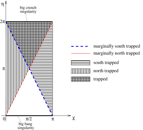
Figure 2: A spacetime diagram of a closed, dust, RW spacetime.

With the line element above, the tangents to the future, radial, south-directed, null geodesics are given by

$$l^{a}=\frac{1}{\sqrt{2}}\Bigg{[}\Big{(}\frac{\partial}{\partial\tau}\Big{)}^{a}+\frac{1}{a(\tau)}\Big{(}\frac{\partial}{\partial\chi}\Big{)}^{a}\Bigg{]}$$ (8)

and the tangents to the north-directed ones are given by

$$n^{a}=\frac{1}{\sqrt{2}}\Bigg{[}\Big{(}\frac{\partial}{\partial\tau}\Big{)}^{a}-\frac{1}{a(\tau)}\Big{(}\frac{\partial}{\partial\chi}\Big{)}^{a}\Bigg{]}$$ (9)

with $l^{a}n_{a}=-1$.

Given a radial null vector field $k^{a}$ its expansion is given by

$$\theta_{(k)}={q^{a}}_{b}\nabla_{a}k^{b}$$ (10)

where $q_{ab}\equiv r^{2}\Big{(}(d\theta)_{a}(d\theta)_{b}+\sin^{2}\theta\,(d\phi)_{a}(d\phi)_{b}\Big{)}$ is the metric on the 2-sphere. A simple calculation yields:

$$\theta_{(l)}=\frac{\sqrt{2}}{a}\big{(}\dot{a}+\cot\chi)\quad\quad\theta_{(n)}=\frac{\sqrt{2}}{a}\big{(}\dot{a}-\cot\chi)$$ (11)

where $\dot{a}\equiv\frac{da}{d\tau}$. Using (6), (7), these can be used to solve for the surfaces $\chi_{(l)}(\eta)$ and $\chi_{(n)}(\eta)$ where the corresponding expansions of null geodesics vanish. The result is:

$$\chi_{(l)}(\eta)=\pi-\frac{\eta}{2}\quad\quad\chi_{(n)}(\eta)=\frac{\eta}{2}$$ (12)

Let the 3-surfaces defined by $\chi(\eta)=\chi_{(l)}(\eta)$ and $\chi(\eta)=\chi_{(n)}(\eta)$ be denoted $\Sigma_{(l)}$ and $\Sigma_{(n)}$ respectively.

A natural question, which, as will be discussed later, is relevant to the construction of the counterexample and further discussions, is whether $\Sigma_{(l)}$ and $\Sigma_{(n)}$ are timelike, null, or spacelike. This is answered in the appendix, where the following result is shown:

Given a RW spacetime of any spatial geometry (closed, flat, or open) and matter satisfying an equation of state of the form $P=\omega\rho$ with $\rho>0$, then the type of $\Sigma_{(l)}$ and $\Sigma_{(n)}$ depends on $\omega$ alone:

$$\Sigma_{(l)}\text{ and }\Sigma_{(n)}\text{ are }\left\{\begin{array}[]{l@{\quad\quad\quad}l}\text{timelike,}&-1<\omega<\frac{1}{3}\\ \text{null,}&\omega=\frac{1}{3},-1\\ \text{spacelike,}&\omega>\frac{1}{3}\text{ or }\omega<-1\end{array}\right.$$

This implies that in the case of dust ($\omega=0$) the surfaces are timelike.  A spacetime diagram of a closed, dust-filled RW spacetime is shown in Fig. 2.

3 Oppenheimer–Snyder-like spacetimes

In 1939, Oppenheimer and Snyder [15] gave the first example of a spacetime that describes the gravitational collapse of matter into a black hole. In their work the matter was a ball of dust (i.e. pressureless, homogeneous fluid), as a model for the gravitational collapse of a neutron star.

One way of constructing new solutions to Einstein’s field equations from known solutions is by matching two portions of two different spacetimes together. The OS-like spacetimes are obtained by matching a part of a dust-filled RW spacetime with a part of a Schwarzschild spacetime. The Israel–Darmois junction conditions [16, 17] are conditions to be imposed on the matching surface, the surface where the two portions are joined, in a way to obtain such a solution. Only a specific case of such matchings will be used—a matching with no extra matter between the two parts matched (i.e. no thin shell of matter) and one where the matching surface is timelike. In this case the junction conditions are equivalent to the 3-metric on the matching surface being the same when evaluated in either portion being matched, and similarly for the extrinsic curvature of this surface in each portion.

Although OS-like spacetimes can be constructed using RW spacetimes of any spatial geometry (closed, flat, or open), the current discussion will be limited to closed RW spacetimes, as these will suffice for the construction of the counterexample and discussion thereafter.

Consider first the original OS model. The discussion follows [14]. (An excellent treatment of the original OS model can be found in [18].)  Two spacetimes are taken: a closed, dust-filled RW spacetime with a line element given by (5) and a Schwarzschild spacetime with the line element

$$ds^{2}=-\Big{(}1-\frac{2M}{R}\Big{)}dt^{2}+\Big{(}1-\frac{2M}{R}\Big{)}^{-1}dR^{2}+R^{2}d\Omega^{2}$$ (14)

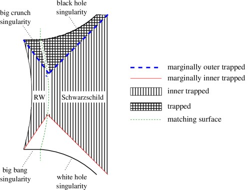
Figure 3: A spacetime diagram of the original OS model.

The RW spacetime is cut at some fixed coordinate $\chi$, $\chi_{0}\leq\frac{\pi}{2}$, and only the northern portion, $\chi\leq\chi_{0}$ is kept. The Schwarzschild spacetime is cut along a surface spanned by radial timelike geodesics at rest at $t=0$ at Schwarzschild coordinate radius $R_{0}\geq 2M$ in Region I of Fig. 1. The portion that contains the asymptotically flat end of Region I is kept. The two portions kept (of RW and Schwarzschild) are pasted together along the surfaces originally used to cut the two spacetimes.

As before, let $a_{m}$ be the maximum value attained by the scale factor $a$. The junction conditions are satisfied and a new spacetime is obtained when [14]

$$R_{0}=a_{m}\sin\chi_{0}$$ (15)

$$M=\frac{1}{2}a_{m}\sin^{3}\chi_{0}$$ (16)

The resulting spacetime includes a white hole singularity continuously joined to a big bang singularity. The ball of matter starts expanding as matter comes out from the white hole. The $t=0$ hypersurface of Schwarzschild, coincides with the maximum expansion of the ball, a moment of time symmetry in the RW region. Finally the ball of matter collapses and a black hole is formed ending in a big crunch singularity continuously joined to a black hole singularity. A spacetime diagram is shown in Fig. 3.

As the matching is done with no thin matter shell, i.e. the extrinsic curvature is the same when evaluated in both portions matched, then the marginally outer/inner trapped surfaces are continuous as can be seen in the spacetime diagram. Note how in this matching the marginally outer (resp. inner) trapped surfaces in Fig. 3 in the RW portion are just the marginally south (resp. north) trapped surfaces in Fig. 2.

A 2-parameter family of solutions is obtained in this manner. One parameter is the total mass of the spacetime, as this can be rescaled by taking $M\to\alpha M$ as well as $\rho\to\alpha\rho$ and $R\to\alpha R$, where $\rho=T_{ab}u^{a}u^{b}$ is the density of matter in the RW region. The other parameter is $\chi_{0}$, or equivalently, given a total mass $M$, at what value of $R_{0}$ the Schwarzschild spacetime is cut. The latter freedom will play an important role in the construction of the counterexample.

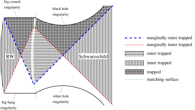
Figure 4: A spacetime diagram of a generalized OS spacetime with $\chi_{0}>\frac{\pi}{2}$.

Figure 5: Embedding diagrams of OS-like spacetimes sliced at the moment of time symmetry. One angular dimension is suppressed by setting $\theta~{}=~{}\pi/2$. Left: a normal OS spacetime. Right: a generalized OS spacetime with $\chi_{0}~{}>~{}\frac{\pi}{2}$.

The construction above can be generalized by dropping the requirement $\chi_{0}\leq\frac{\pi}{2}$. This adds spacetimes with a “star inside the black hole”, i.e. the dust RW region never gets to Region I of the Schwarzschild spacetime. Instead the surface of matching passes through the other side of the Schwarzschild wormhole, Region III. This corresponds to taking $\chi_{0}>\frac{\pi}{2}$ as well as cutting the Schwarzschild spacetime using geodesics that at the moment of time symmetry are located at Schwarzschild coordinate radius $R_{0}$ (with $R_{0}>2M$) in Region III of Fig. 1. The portion to be kept in each spacetime is the same, i.e. keeping the portion $\chi\leq\chi_{0}$ in the RW spacetime and keeping the portion of Schwarzschild that contains the asymptotically flat end in Region I. The junction conditions are unchanged as well and take the form (15), (16).

A spacetime diagram of the resulting spacetime is shown in Fig. 4. An embedding diagram of both a normal OS spacetime and a generalized one with $\chi_{0}>\frac{\pi}{2}$ is shown in Fig. 5.

4 A counterexample to the apparent horizon Penrose inequality

The counterexample is obtained by taking a portion of a generalized OS spacetime and matching it further. After the RW portion of this generalized OS spacetime comes a second Schwarzschild region, with a bigger mass parameter. It is then possible to slice this spacetime with a spacelike surface and get initial data that provides a counterexample. A spacetime diagram of such a construction is shown in Fig. 6 and the precise details are now described.

The construction is obtained by matching the following portions:

1. A Schwarzschild spacetime with mass $M$ is cut along a surface spanned by radial timelike geodesics at rest at $t=0$ at Schwarzschild coordinate radius $R_{0}>2M$ in Region III of Fig. 1. The portion that contains the asymptotically flat end of Region I is kept. This is the right Schwarzschild region in Fig. 6.

2. A closed, dust-filled RW spacetime with $a_{m}$ being the maximum value attained by its scale factor. This spacetime is cut along two surfaces of fixed $\chi$, i.e. $\chi=\chi_{0}$ and $\chi=\chi_{1}$, with $\frac{\pi}{2}\leq\chi_{1}<\chi_{0}<\pi$ (thus dividing this spacetime into 3 separate regions). The portion kept for the purposes of matching is the region $\chi_{1}\leq\chi\leq\chi_{0}$. This is the right RW region in Fig. 6.

3. A second Schwarzschild spacetime, this time with mass $M_{1}$, is cut along 2 surfaces (dividing it as well into 3 separate regions). The first cut is along a surface spanned by radial timelike geodesics at rest at $t=0$ at Schwarzschild coordinate radius $R_{1}\geq 2M_{1}$ in Region III of Fig. 1, and the second cut is along another surface spanned by radial timelike geodesics that are at rest at $t=0$ at Schwarzschild coordinate radius $R_{2}>R_{1}$ in Region III of Fig. 1. The portion kept is the middle one. This is the left Schwarzschild region in Fig. 6.

4. A second closed, dust-filled RW spacetime, this time with $a^{\prime}_{m}$ being the maximum value attained by its scale factor. This spacetime is cut along a surface of fixed $\chi$, $\ \frac{\pi}{2}<\chi_{2}<\pi$ keeping the portion $\chi\leq\chi_{2}$. This is the left RW region in Fig. 6.

The portions are matched together in consecutive order, i.e. 1-2-3-4, as can be seen in Fig. 6. The exact details of these matchings are:

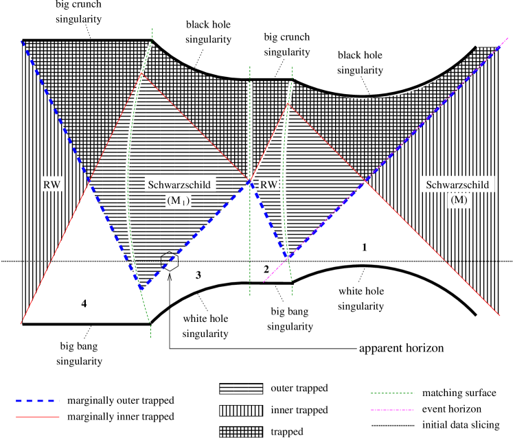
Figure 6: A spacetime diagram of a counterexample to the apparent horizon Penrose inequality. Notice how the slice passes just below the event horizon in Portion 1. Therefore, the apparent horizon is located where the initial data intersects the marginally outer trapped 2-spheres in the second Schwarzschild region, Portion 3.

First, the matching of Portion 1 and 2. Portion 1 is matched along the original surface used to obtain it. Portion 2 is matched along the surface spanned by $\chi=\chi_{0}$. The junction conditions are satisfied when

$$R_{0}=a_{m}\sin\chi_{0}$$ (17)

$$M=\frac{1}{2}a_{m}\sin^{3}\chi_{0}$$ (18)

This is the same matching as in a generalized OS spacetime with $\chi_{0}>\frac{\pi}{2}$.

Next, the matching of Portion 2 and 3. Portion 2 is matched along the surface spanned by $\chi=\chi_{1}$. Portion 3 is matched along the surface with geodesics passing at $R_{1}$ at $t=0$. The junction conditions for this matching are satisfied when

$$R_{1}=a_{m}\sin\chi_{1}$$ (19)

$$M_{1}=\frac{1}{2}a_{m}\sin^{3}\chi_{1}$$ (20)

Finally, the matching of Portion 3 and 4. Portion 3 is matched along the surface with geodesics passing at $R_{2}$ at $t=0$. Portion 4 is matched along the surface spanned by $\chi=\chi_{2}$. The junction conditions are satisfied when

$$R_{2}=a^{\prime}_{m}\sin\chi_{2}$$ (21)

$$M_{1}=\frac{1}{2}a^{\prime}_{m}\sin^{3}\chi_{2}$$ (22)

A choice of all these parameters satisfying the junction conditions uniquely determines the spacetime. However, there is freedom in choosing the parameters leading to a 4-parameter family of spacetimes constructed in this way: Choose any $M$ and any $\chi_{0}\in(\frac{\pi}{2},\pi)$. This uniquely determines $R_{0}$ and $a_{m}$ by (17),(18). A choice of any $\chi_{1}\in[\frac{\pi}{2},\chi_{0})$ now uniquely determines $M_{1}$ and $R_{1}$ by (19),(20). Finally a choice of any $R_{2}>R_{1}$ uniquely determines $a^{\prime}_{m}$ and $\chi_{2}$ by (21),(22).

Certain members of this 4-parameter family of spacetimes contain slices that are counterexamples to the apparent horizon Penrose inequality as will now be demonstrated.

Given any $M$ and any $\chi_{0}\in(\frac{\pi}{2},\pi)$ choose $\chi_{1}$ in its allowed range, i.e. $\chi_{1}\in[\frac{\pi}{2},\chi_{0})$. (In Fig. 6, $\chi_{1}=\frac{\pi}{2}$.)  This determines $M_{1}$ and $R_{1}$. It remains to choose $R_{2}$ as long as $R_{2}>R_{1}$. Later it will turn out that a counterexample is obtained as long as $R_{2}$ is large enough, thus such a choice can then be made.

The initial data is obtained by taking the following slice: In Portion 1, part of a Schwarzschild spacetime, the slice is at constant Kruskal-Szekeres coordinate T (i.e. it is a horizontal slice in a Kruskal diagram). It is chosen so as to pass just below the event horizon in Portion 1 (see Fig. 6). In Portion 2, part of a RW spacetime, the slice continues at fixed $\eta$. In Portion 3, part of another Schwarzschild spacetime, the slice continues, again, at fixed T. In Portion 3, the slice intersects the 3-surface corresponding to the event horizon of the Schwarzschild spacetime from which this portion originates. This intersection is a marginally outer trapped 2-sphere. Finally in Portion 4, part of a RW spacetime, the slice continues at fixed $\eta$.

In order to guarantee that this slice contains such a marginally outer trapped 2-sphere in Portion 3, $R_{2}$ must be chosen in such a way that Portion 4 will start “further back”. This is satisfied if $R_{2}$ is large enough; thus, a suitable value of $R_{2}$ is now chosen.

In this initial data, the apparent horizon, the outermost marginally outer trapped surface, is just that marginally outer trapped 2-sphere in Portion 3, as no surface outside it is marginally outer trapped. The area of the apparent horizon, in this case, is therefore given by

$$A=4\pi(2M_{1})^{2}$$ (23)

whereas, in contrast, the total (ADM) mass of this initial data is $M$, as this is evaluated in the asymptotically flat region. As $\chi_{1}\in[\frac{\pi}{2},\chi_{0})$ then $\sin\chi_{1}>\sin\chi_{0}$ and then from (18),(20) it follows that

$$M_{1}>M$$ (24)

Finally, (23),(24) imply:

$$M<\sqrt{A/16\pi}$$ (25)

This is an asymptotically flat spacetime satisfying the dominant energy condition. It is spherically symmetric with a spherically symmetric slice yielding initial data that violates the apparent horizon Penrose inequality. Furthermore, as $\chi_{0}$ can be chosen to be arbitrarily close to $\pi$, $\sin\chi_{0}$ can be made as small as one wishes and therefore $A$ can be made as large as one wishes. Thus, for all $\epsilon>0$ there exists a spacetime and a slice as described above producing initial data with $M<\epsilon\sqrt{A/16\pi}$ with $A$ the area of the apparent horizon, i.e. the inequality can be violated to an arbitrarily large extent.

The fact that $M_{1}$ is bigger than $M$, so that this construction can work as a counterexample to the apparent horizon Penrose inequality, is due to specific features of Portion 2. As $\Sigma_{(l)}$ in that portion is foliated by marginally outer trapped 2-spheres, one can define $A(\eta)$ to be the area of these 2-spheres. Using (6),(12), this is found to be

$$A(\eta)=4\pi\,a^{2}(\eta)\sin^{2}\chi_{l}(\eta)=\frac{\pi}{2}a_{m}^{2}(1-\cos\eta)^{3}$$ (26)

Thus, this area increases during the expansion ($0\leq\eta<\pi$) of the RW portion and decreases during its collapse ($\pi<\eta\leq 2\pi$). As the matching of Portions 1 and 2 and then that of Portions 2 and 3 is such that $\Sigma_{(l)}$ in Portion 2 is limited to an expanding RW region,  the area of marginally outer trapped 2-spheres in this portion is growing. It is this bigger area that implies a bigger mass parameter, $M_{1}$, in Portion 3.

5 Quasi-local constructions

Before remarking on various versions of the Penrose inequality, it is important to discuss an issue raised by $\Sigma_{(l)}$ being a timelike surface in all the constructions above.

In recent years certain quasi-local constructions were suggested as either useful in applications pertaining to the dynamics of black holes or even as candidates to replace event horizons altogether as their boundaries. Recently, Ashtekar and Krishnan [11] defined and discussed dynamical horizons, building on previous formulations of isolated horizons [19] and Hayward’s [20] notion of trapping horizons. The following definitions follow the works where they were originally defined.

A dynamical horizon is a smooth, three-dimensional, spacelike sub-manifold that can be foliated by a family of closed 2-surfaces with the expansion of future-directed null geodesics normal to these 2-surfaces vanishing in one direction and strictly negative in the other.

A future outer trapping horizon is the closure of a 3-surface foliated by 2-surfaces on which: The expansion of future-directed null geodesics normal to the 2-surface in one direction vanishes, denote it as $\theta_{(+)}$. The expansion in the other direction, $\theta_{(-)}$, is strictly negative, and finally $\mathcal{L}_{-}\theta_{+}$ is also strictly negative.

In asymptotically flat spacetimes both dynamical horizons and future outer trapping horizons are 3-surfaces that are foliated by marginally outer trapped surfaces. Moreover, dynamical horizons are spacelike by definition, and future outer trapping horizons must be spacelike or null [11]. In contrast, in all of the spacetimes constructed here, the 3-surfaces foliated by marginally outer trapped 2-spheres are never spacelike. They are null in the Schwarzschild portions and are timelike where there is matter and dynamics, i.e. in the RW portions. This raises the issue of whether dynamical horizons or future outer trapping horizons are associated, generically, with gravitational collapse.

Given a 3-surface foliated by marginally outer trapped surfaces, Ashtekar and Krishnan [11] show that the question whether the 3-surface is timelike or spacelike is directly related to $\mathcal{L}_{n}\theta_{(l)}$, the derivative of the expansion of future, outgoing, null geodesics normal to the 2-surfaces in the direction of ingoing ones. If the 3-surface is not null and if $\mathcal{L}_{n}\theta_{(l)}$ is non-zero, then they show, using the Raychaudhuri equation, that the 3-surface is spacelike if $\mathcal{L}_{n}\theta_{(l)}$ is negative and it is timelike if $\mathcal{L}_{n}\theta_{(l)}$ is positive. Thus, the issue translates to whether $\mathcal{L}_{n}\theta_{(l)}$ is generically positive or negative.

Ashtekar and Krishnan [11] provide arguments for $\mathcal{L}_{n}\theta_{(l)}$ to be generically negative, and similarly Hayward [21] provides an argument for future outer trapping horizons to be generic. However, none of these arguments seem satisfactory.

As a concrete example of dynamical horizons Ashtekar and Krishnan [11] provide the Vaidya spacetimes. The OS spacetimes provide a concrete example where a 3-surface, foliated by marginally outer trapped surfaces, is timelike. Both the Vaidya and OS spacetimes are spherically symmetric, and in spherical symmetry the issue of whether such a 3-surface is spacelike or timelike, can be further explored via the Newman–Penrose formalism [22].

The work of Newman and Penrose involves a spinor formalism for general relativity. In [22] Newman and Penrose take two null vectors, $l^{a}$, $n^{a}$ with normalization $l^{a}n_{a}=-1$. With respect to some scalar quantity $\phi$ they define in (2.12) $\Delta\phi=n^{a}\nabla_{a}\phi$ and the spin coefficient $\rho$ is a function defined in (4.1a) such that $\rho=\frac{1}{2}\theta_{(l)}$. Thus, up to a numerical factor, $\Delta\rho$ is $\mathcal{L}_{n}\theta_{(l)}$, hence equation (4.2q) is useful.

In the spherical symmetric case and on the marginally outer trapped surface, where $\rho=0$, most terms in (4.2q) vanish and it reduces to

$$\Delta\rho=-\psi_{2}-2\Lambda$$ (27)

As $\psi_{2}$ is, up to a numerical factor, a component of the Weyl tensor and $\Lambda$ is, up to a numerical factor, $R$, the scalar curvature, this becomes

$$\mathcal{L}_{n}\theta_{(l)}=C_{abcd}\,l^{a}n^{b}\,l^{c}\,n^{d}+\frac{R}{6}$$ (28)

In this form it is easier to see how $\mathcal{L}_{n}\theta_{(l)}$ is positive in one case and is negative in the other.

The Vaidya spacetime is one that contains a null fluid. As a result of this form of stress energy, the scalar curvature in this case vanishes. Hence, in the ingoing Eddington-Finkelstein coordinates used by Ashtekar and Krishnan (28) becomes

$$\mathcal{L}_{n}\theta_{(l)}=C_{abcd}\,l^{a}n^{b}\,l^{c}\,n^{d}=C_{vrvr}=-\frac{1}{r^{2}}$$ (29)

This shows, in agreement with a direct evaluation of the LHS as in [11], that in the Vaidya spacetime $\mathcal{L}_{n}\theta_{(l)}$ is negative, and the 3-surface foliated by marginally outer trapped 2-surfaces is indeed spacelike where the stress-energy is non-vanishing [11].

In the case of a RW spacetime, the non-vacuum portion of an OS spacetime, the Weyl tensor vanishes.  Thus, in this case, (28) becomes

$$\mathcal{L}_{n}\theta_{(l)}=\frac{R}{6}$$ (30)

In the RW spacetime $R=8\pi(\rho-3P)$ so that in the case of dust $R>0$. Consequently $\mathcal{L}_{n}\theta_{(l)}>0$, implying that $\Sigma_{(l)}$ is timelike, in agreement with the result shown in the appendix.

Normal matter satisfies $0\leq P\leq\frac{1}{3}\rho$ and hence the contribution from the scalar curvature should generically be positive. As for the Weyl tensor, it does not seem clear what sign this component should generically have. Nor is it clear what the relation is, if any, between the Weyl tensor and the scalar curvature—which one generically dominates?  Note however, that the above results hold only in the spherically symmetric case. In a non-spherically-symmetric spacetime (4.2q) in [22] will have additional non-vanishing terms and it is therefore much harder to make a precise statement in the general case. Furthermore, in the non-spherically-symmetric case there is no reason to expect $\mathcal{L}_{n}\theta_{(l)}$ to have a constant sign over the entire marginally outer trapped surface.

6 Discussion

Though the counterexample above shows that the apparent horizon Penrose inequality does not hold, it does not contradict the Penrose inequality and it therefore has no effect on the status of the cosmic censorship conjecture.

In the spherically symmetric case, Malec and Ó Murchadha [23] considered another version of the Penrose inequality. Given a spherically symmetric initial data surface, one can not only locate the apparent horizon in it, but also the past apparent horizon (the apparent horizon with respect to past-directed null geodesics).  Define the outermost horizon to be the outermost of the future and past apparent horizons. Malec and Ó Murchadha’s version of the Penrose inequality, which in the present work will be referred to as the outermost horizon Penrose inequality, is that given a spherically symmetric initial data satisfying the dominant energy condition then

$$M\,\geq\,\sqrt{A_{o.h}/16\pi}$$ (31)

with $M$ the total mass and $A_{o.h}$ the area of the outermost horizon.

In [23], Malec and Ó Murchadha proved the outermost horizon Penrose inequality for maximal slices.  This was later proven without requiring maximal slices by Iriondo, Malec, and Ó Murchadha [24] and independently by Hayward [25, 26].

The proofs of the outermost horizon Penrose inequality may suggest that some version of it may hold for initial data lacking spherical symmetry. In such initial data the (future) apparent horizon may not lie completely outside or completely inside the past apparent horizon. The future and past apparent horizons may then intersect in a complicated manner, in which case care must be taken in defining the outermost horizon in initial data without spherical symmetry. One might consider the union of the (future) trapped region and the past trapped region and define the outermost horizon to be the outermost boundary of this union. This, however, will yield a surface that in general need not be smooth.

Another approach to generalizing the formulation of the outermost horizon Penrose inequality to non-spherically-symmetric initial data might be to restrict consideration to the case where the apparent horizon lies completely outside the past apparent horizon, i.e., to formulate the outermost horizon Penrose inequality only in the case where there are no past outer trapped surfaces outside the apparent horizon.  However, it is possible that a spacetime like the one presented in this work can serve as a counterexample for this case as well using a highly non-spherically-symmetric slice, similar to that used in [27]. In this case coming from the asymptotically flat end, the north pole of the 2-spheres might be taken to get very close to the white hole singularity, while the south pole of the 2-spheres does not. Further inside, the slice will approach the spherically symmetric slice shown in Fig. 6. In this way it may be possible to obtain a slice that does not contain any past outer trapped surfaces outside the apparent horizon and in addition, if the apparent horizon is located in the first RW portion or the second Schwarzschild portion, its area might be large enough so as to obtain a counterexample.

It is important to realize that the outermost horizon Penrose inequality actually implies the Penrose inequality in spherical symmetry. In this case $M\geq\sqrt{A_{o.m.}/16\pi}$ with $A_{o.m.}$ the area of the outermost horizon. However, the outermost horizon either coincides with, or lies outside of the apparent horizon. In either case it follows immediately that $M\geq\sqrt{\mathcal{A}/16\pi}$ with $\mathcal{A}$ the minimum area required to enclose the apparent horizon. Thus, in spherical symmetry the “true” Penrose inequality has been proven, and it would be of great interest to extend this to the general case.

Acknowledgments

It is a pleasure to thank Robert M. Wald for guidance and a lot of useful advice along the way, not to mention suggesting this project in the first place. I would also like to thank Mike Seifert, Stefan Hollands, and Piyush Kumar for many useful discussions and suggestions. This research was supported in part by NSF grant PHY 00-90138 to the University of Chicago.

Appendix A The type of $\Sigma_{(l)}$ and $\Sigma_{(n)}$

The line element of a Robertson–Walker spacetime is given by

$$ds^{2}=-d\tau^{2}+a^{2}(\tau)\Big{(}dr^{2}+f(r)^{2}d\Omega^{2}\Big{)}$$ (32)

with $f(r)$, depending on the spatial geometry, given by

$$\left\{\begin{array}[]{l@{\quad\quad\quad}l}\sin r,&\text{closed (}k=1\text{) geometry}\\ r,&\text{flat (}k=0\text{) geometry}\\ \sinh r,&\text{open (}k=-1\text{) geometry}\\ \end{array}\right.$$

The spacetime is assumed to have a stress energy tensor of a perfect fluid form with an equation of state $P=\omega\rho$ with $\rho>0$.

The Friedman equations, the field equations applied to such spacetimes are given [4] by

$$3\dot{a}^{2}/a^{2}=8\pi\rho-3k/a^{2}$$ (34)

$$3\ddot{a}/a=-4\pi(\rho+3P)$$ (35)

The 3-surfaces $\Sigma_{(l)}$ and $\Sigma_{(n)}$ are given by $r=r(\tau)$ where the expansion of the relevant geodesics vanish. The radial tangents to this surface are found to be

$$u^{a}=\Big{(}\frac{\partial}{\partial\tau}\Big{)}^{a}\pm\frac{\ddot{a}}{\dot{a}^{2}+k}\Big{(}\frac{\partial}{\partial r}\Big{)}^{a}$$ (36)

Hence

$$u^{a}u_{a}=\Big{(}\frac{\ddot{a}a}{\dot{a}^{2}+k}\Big{)}^{2}-1=\Big{(}\frac{\rho+3P}{2\rho}\Big{)}^{2}-1$$ (37)

where in the last equality, (34) and (35) have been used.

It follows that $u^{a}$, and therefore the 3-surface, is

$$\left\{\begin{array}[]{l@{\quad\quad\quad}l}\text{timelike,}&-1<\omega<\frac{1}{3}\\ \text{null,}&\omega=\frac{1}{3},-1\\ \text{spacelike,}&\omega>\frac{1}{3}\text{ or }\omega<-1\end{array}\right.$$

This is independent of the spatial geometry of the RW model.

References

- [1] R. Penrose, Ann. New York Acad. Sci. 224, 125 (1973).
- [2] P. S. Jang and R. M. Wald, J. Math. Phys. 18, 41 (1977).
- [3] S. W. Hawking, Phys. Rev. Lett. 26, 1344 (1971).
- [4] R. M. Wald, General Relativity (University of Chicago Press, Chicago, 1984).
- [5] H. Bray and P. Chrusciel, gr-qc/0312047.
- [6] G. Huisken and T. Ilmanen, J. Diff. Geom. 59, 353 (2001).
- [7] R. Geroch, Ann. New York Acad. Sci. 224, 108 (1973).
- [8] H. Bray, J. Diff. Geom. 59, 177 (2001).
- [9] E. Malec, M. Mars, and W. Simon, gr-qc/0212040.
- [10] L. Szabados, Living Rev. Relativity 7, (2004), 4. [Online article]: cited on 8/11/04, http://www.livingreviews.org/lrr-2004-4
- [11] A. Ashtekar and B. Krishnan, Phys. Rev. D 68, 104030 (2003).
- [12] J. Karkowski, P. Koc, and Z. Swierczynski, Class. Quant. Grav. 11, 1535 (1994).
- [13] J. Frauendiener, Phys. Rev. Lett. 87, 101101 (2001).
- [14] C. W. Misner, K. S. Thorne, and J. A. Wheeler, Gravitation (W.H. Freeman and Co., San Francisco, 1973).
- [15] J. R. Oppenheimer and H. Snyder, Phys. Rev. 56, 455 (1939).
- [16] W. Israel, Nuovo Cimento B44, 1 (1966). Erratum: B48, 463 (1967).
- [17] G. Darmois, Memorial des Sciences Mathematics XXV (Gauthier-Villars, Paris, 1927).
- [18] E. Poisson, A Relativist’s Toolkit (Cambridge University Press, New York, 2004).
- [19] A. Ashtekar, C. Beetle, and S. Fairhurst, Class. Quant. Grav. 17 253 (2000).
- [20] S. A. Hayward, Phys. Rev. D 49, 6467 (1994).
- [21] S. A. Hayward, gr-qc/0008071.
- [22] E. Newman and R. Penrose, J. Math. Phys. 3, 566 (1962). Errata 4, 998 (1963).
- [23] E. Malec and N. Ó Murchadha, Phys. Rev. D 49, 6931 (1994).
- [24] M. Iriondo, E. Malec, and N. Ó Murchadha, Phys. Rev. D 54, 4792 (1996).
- [25] S. A. Hayward, Phys. Rev. D 53, 1938 (1996).
- [26] S. A. Hayward, Phys. Rev. Lett. 81, 4557 (1998).
- [27] R. M. Wald and V. Iyer, Phys. Rev. D 44, R3719 (1991).