Entropy of gravitationally collapsing matter in FRW universe models

Abstract

We look at a gas of dust and investigate how its entropy evolves with time under a spherically symmetric gravitational collapse. We treat the problem perturbatively and find that the classical thermodynamic entropy does actually increase to first order when one allows for gravitational potential energy to be transferred to thermal energy during the collapse. Thus, in this situation there is no need to resort to the introduction of an intrinsic gravitational entropy in order to satisfy the second law of thermodynamics.

I Introduction

Today there is broad consensus among cosmologists that the configuration of energy in the early universe was very homogeneous and isotropic. Observations of the temperature variations in the cosmic microwave radiation have also shown that the Universe was in a state close to thermodynamic equilibrium $400\,000$ years after Big Bang, with relative temperature and density variations of the order $10^{-5}$ Spergel et al. (2003).

Naively, one expects the entropy in a gas to be higher the more homogeneously distributed its density and temperature is. Thus, the early universe described above should be one of near maximal entropy, since it differs only by a small fraction from one of total homogeneity in density and temperature. However, due to gravity, small inhomogeneities start to grow and eventually end up forming structures such as galaxies, stars, planets, planetary clouds etc. This evolution is in the direction of greater inhomogeneities both in energy density and temperature, which according to the argument above, appears to violate the second law of thermodynamics by decreasing the entropy. Obviously, something must be wrong with this picture, since we consider the second law of thermodynamics to be a basic law of physics and it should therefore not be violated.

A possible solution to this apparent paradox comes from considering the quantity known as gravitational entropy. This was introduced by R. Penrose in the 1977 in connection with his study of the properties of the initial singularity of the universe Penrose (1977, 1979, 1981). It is a quantity which can be interpreted as an entropy intrinsic to the gravitational field. It takes into account the attractive nature of gravity and increases as a gas collapses under the influence of gravity. This allows one to define a general entropy which is the sum of the ordinary thermodynamic entropy and this new gravitational entropy. If the sum of the two types of entropy increases during gravitational collapse of a gas, the second law of thermodynamics will then be preserved.

In this paper we will show that the thermodynamics entropy of a collapsing gas does actually increase, which allows us to explain the collapse without introducing the gravitational entropy. We look at a perturbed ideal gas in a FRW background and consider changes in its classical entropy up to first order in the energy density. We find that the increase in the thermal energy which comes from potential energy released in the collapse actually makes the total thermodynamic entropy increase, even though the temperature inhomogeneity increases.

The structure of this paper is as follows. In section 2 we look at a simplified model consisting of ideal particles in a box and explain why one would expect the thermodynamic entropy to decrease as the inhomogeneities increase. In section 3 we introduce a tool which we will need when considering the growth of small inhomogeneities, namely cosmological perturbation theory. In section 4 we derive an expression for the thermodynamic entropy of a gas in an expanding universe. In section 5 we specialize to spherically symmetric collapsing gases and arrive at our main result. Finally, section 6 contains a summary and our conclusion.

II Simple picture: Ideal gas in a box

In this section we look at gas confined to a box and show that its entropy is maximal when the density is homogeneous and the temperature is the same everywhere.

Consider an isolated box that is divided into two chambers of equal volume. Each of these contains a gas of the same type of particles with different temperatures and densities, as illustrated in Fig. 1. We will look at two different scenarios: 1) when the temperature in the chambers is the same but the density is different. And 2) when temperature is different, while the density is the same. We then compare these to a third scenario, in which we remove the wall between the two chambers so that we have only one gas with just one temperature and one density.

First, we need the expression for the entropy of an ideal gas consisting of $N$ ideal particles in a volume $V$ Kittel and Kroemer (1980),

$$S_{\mbox{\tiny{ideal}}}=Nk_{B}\ln{\left[\frac{V}{N}\left(\frac{mk_{B}T}{2\pi\hbar^{2}}\right)^{3/2}e^{5/2}\right]}\,.$$ (1)

Figure 1: An isolated box consisting of two separated chambers with particles of different temperatures and densities.

Let us look at the third scenario first. Let $T$ be the temperature in the gas and $N$ the total amount of particles in the box. The entropy in the box in this scenario, which represents the totally homogeneous case, is then

$$S_{3}=Nk_{B}\ln{\left[\frac{KT^{3/2}V}{N}\right]}\,,$$ (2)

where we have defined the constant

$$K=\left[\frac{mk_{B}Te^{5/3}}{2\pi\hbar^{2}}\right]^{3/2}.$$ (3)

How does the entropy differ from this in the other two, inhomogeneous scenarios? In the first scenario the temperatures are the same, but the number of particles in the two chambers is different. The total number of particles is conserved, so we have that $N_{1}+N_{2}=N$, where $N_{1}$ and $N_{2}$ are the numbers of particles in the two chambers respectively. Furthermore, we assume that the two chambers have the same volume $V/2$. The total entropy in the box is then the sum of the entropies in the two chambers:

$$S_{1} =N_{1}k_{B}\ln{\left[\frac{KT^{3/2}V}{2N_{1}}\right]}+N_{2}k_{B}\ln{\left[\frac{KT^{3/2}V}{2N_{2}}\right]}$$

$$=Nk_{B}\ln{\frac{KT^{3/2}V}{2}}-\left(N_{1}k_{B}\ln{N_{1}}+N_{2}k_{B}\ln{N_{2}}\right)$$ (4)

A transition from the totally homogeneous scenario to this results in an entropy difference which is

$$\Delta S=S_{1}-S_{3}=-Nk_{B}\bigg{(}\ln{2}+x\,\ln{x}+(1-x)\ln{(1-x)}\bigg{)}\,,$$ (5)

where we have defined $x\equiv N_{1}/N$. We can restrict $x$ to the interval $0<x<1/2$ without any loss of generality. It is then a simple task to verify that $\Delta S<0$. Thus, based on this simple picture, we can conclude that an increase in inhomogeneity of the density of an ideal gas leads to a reduction of the entropy.

Now, let us look at the second scenario, where there is a temperature difference between the two chambers which both contain the same amount of particles, $N/2$. The temperatures of the two chambers are $T_{1}$ and $T_{2}$ respectively. The total entropy of the box in this scenario is

$$S_{2}=Nk_{B}\left(\ln{\frac{KV}{N}}+\frac{3}{4}\ln{(T_{1}T_{2})}\right)\,.$$ (6)

If we imagine the gas first being in the totally homogeneous state of scenario 3 and then changing into the thermally inhomogeneous state of scenario 2, the entropy difference will be

$$\Delta S=\frac{3Nk_{B}}{4}\ln{\frac{T_{1}T_{2}}{T^{2}}}\,.$$ (7)

Assume now that the thermal energy is conserved in this transition, i.e. that the average temperatures in the two scenarios are the same. This means that $T_{1}+T_{2}=2T$. Under this assumption, when does this entropy difference become non-negative? We see that this will be the case when

$$\frac{4T_{1}T_{2}}{(T_{1}+T_{2})^{2}}\geq 1\quad\mbox{ i.e. }\quad(T_{1}-T_{2})^{2}\leq 0\,.$$ (8)

This is only satisfied when $T_{1}=T_{2}=T$, in which case there will be an equality between the left and the right hand side. If $T_{1}$ and $T_{2}$ are different, i.e. there is a temperature difference between the two chambers, the entropy difference in (7) will be negative. Thus, an increase in temperature inhomogeneity will result in a decrease in the entropy.

However, we must not forget that we have assumed that the thermal energy is conserved, just as we assumed that the particle number is conserved. For this simple example of particles in an isolated box both these assumptions will be true. For a gravitationally collapsing gas, however, this need not be true. The total mass, which is the equivalent of the total particle number in the box example, must obviously be conserved so we should expect the entropy to decrease as the energy density becomes more inhomogeneous. But the thermal energy will not be conserved as the gas undergoes a gravitational collapse. As the energy density near the overdensity increases, the potential energy of the inward falling portions of the gas is converted to thermal energy. In other words, there will be an increase in the thermal energy of the gas, which tends to increase the entropy.

To summarize, the entropy change in a gravitationally collapsing gas can be ascribed to two different effects, namely a decrease due to increasing density and temperature inhomogeneities and an increase due to increasing temperature. As we will show, using first order perturbation theory, the sum of these two effects yields an increasing total entropy when one assumes that all the loss in potential energy is converted into thermal energy.

We start by reviewing the basics of scalar perturbation theory.

III Scalar perturbation theory

We will only consider scalar perturbations since these are the only ones that give rise to gravitational collapse. For a more detailed review of perturbation theory, the interested reader is referred to the standard references Mukhanov et al. (1992); Ma and Bertschinger (1995); Brandenberger (2004). We assume that the universe is occupied by matter in the form of a perfect fluid with no anisotropic stress. The energy density inhomogeneity is described as a linear perturbation to a flat, matter dominated FRW universe. This allows us to write the perturbed metric in terms of only one perturbing function $\Phi$, the so-called Bardeen potential:

$$ds^{2}=a^{2}(\eta)\left\{(1+2\Phi)d\eta^{2}-(1-2\Phi)\delta_{ij}dx^{i}dx^{j}\right\}\,,$$ (9)

where $\eta$ is conformal time and $a$ is the scale factor of the universe.

The energy-momentum tensor for the matter content is written as a homogeneous zeroth order term plus a non-homogeneous first order perturbation:

$$T^{\mu}_{\nu}=^{(0)}\!\!T^{\mu}_{\nu}+\delta T^{\mu}_{\nu}\,.$$ (10)

Using the definition for the energy-momentum tensor of a perfect fluid, the equation of state for matter, and the four-velocity identity $u^{\mu}u_{\mu}=1$, we can write the components as:

$${}^{(0)}\!T^{0}_{0} =\rho_{0} \delta T^{0}_{0} =\delta\rho$$ (11)

$${}^{(0)}\!T^{0}_{i} =0 \delta T^{0}_{i} =-\rho_{0}a\delta u^{i}$$ (12)

$${}^{(0)}\!T^{i}_{j} =0 \delta T^{i}_{j} =0$$ (13)

where $\rho_{0}$ is the average density of the fluid, $\delta\rho$ is the density perturbation and $\delta u^{i}$ the velocity perturbation. In the expressions above and throughout this paper we use the convention that Latin indices run over spatial components only, while Greek indices run over both space and time components.

We require the Einstein equation for the fluid to be satisfied independently for each order in the perturbation. This gives us the following zeroth order equations

$$\mathcal{H}^{2}=\frac{8}{3}\pi Ga^{2}\rho_{0}$$ (14)

and

$$\mathcal{H}^{2}+2\dot{\mathcal{H}}=0\,,$$ (15)

where $\mathcal{H}=\frac{1}{a}\frac{da}{d\eta}$ and the dot denotes differentiation with respect to $\eta$. The first order equations are

$$\nabla^{2}\Phi-3\mathcal{H}(\dot{\Phi}+\mathcal{H}\Phi)=\frac{3}{2}\mathcal{H}^{2}\delta$$ (16)

$$\left\{\dot{\Phi}+\mathcal{H}\Phi\right\}_{,i}=-\frac{3}{2}\mathcal{H}^{2}a\delta u^{i}$$ (17)

$$\ddot{\Phi}+3\mathcal{H}\dot{\Phi}+(\mathcal{H}^{2}+2\dot{\mathcal{H}})\Phi=0$$ (18)

where we have defined the density contrast as $\delta\equiv\delta\rho/\rho_{0}$, and $A_{,j}\equiv\frac{\partial A}{\partial x^{j}}$. The zeroth order equations are the ordinary FRW equations for a matter dominated, flat universe expressed in conformal time instead of the usual comoving time. The solution to these equations is

$$a=\left(\frac{\eta}{\eta_{0}}\right)^{2}\,\quad\mbox{and}\,\quad\rho_{0}=\rho_{00}\left(\frac{\eta_{0}}{\eta}\right)^{6}\,,$$ (19)

where we have defined $\eta_{0}$ such that $a(\eta_{0})=1$, and $\rho_{00}$ is the energy density at $\eta=\eta_{0}$, which can be written as

$$\rho_{00}=\frac{3}{2\pi G\eta_{0}^{2}}\,.$$ (20)

We shall later need the relation between conformal and comoving time. Using the definition $a(\eta)d\eta=dt$, we can write this as

$$\eta=\eta_{0}\left(\frac{t}{t_{0}}\right)^{\frac{1}{3}}\,,$$ (21)

where $t_{0}$ is the initial comoving time that corresponds to $\eta_{0}$. These are related via the expression

$$t_{0}=\frac{\eta_{0}}{3}\,.$$ (22)

Let us introduce a new dimensionless time parameter $\tau$, which measures time relative to the initial time $t_{0}$, i.e.

$$\tau\equiv\frac{t-t_{0}}{t_{0}}\,.$$ (23)

Using this new time parameter we can write the scale factor and the unperturbed energy density as

$$a(\tau)=(1+\tau)^{\frac{2}{3}}\,\quad\mbox{and}\,\quad\rho_{0}(\tau)=\rho_{00}(1+\tau)^{-2}\,.$$ (24)

Next, we solve the first order equations. We start with equation (18), which doesn’t couple to the other two equations, and obtain the metric perturbation $\Phi$. The remaining perturbing functions $\delta$ and $\delta u^{i}$ are then obtained by a simple substitution of $\Phi$ into equations (16) and (17). Disregarding solutions that decrease with time, we can write the perturbations as:

$$\Phi(\mathbf{x},\tau) =f(\mathbf{x})$$ (25)

$$\delta(\mathbf{x},\tau) =\frac{1}{6}\eta_{0}^{2}(1+\tau)^{2/3}\,\nabla^{2}f(\mathbf{x})-2f(\mathbf{x})$$ (26)

$$\delta u^{i}(\mathbf{x},\tau) =-\frac{\eta_{0}}{3}\frac{df(\mathbf{x})}{dx^{i}}(1+\tau)^{-1/3}$$ (27)

where $f(\mathbf{x})$ is an arbitrary function of spatial coordinates only. In order for these perturbations to be physically acceptable they must vanish at infinity, i.e.

$$\lim_{\|\mathbf{x}\|\to\infty}f(\mathbf{x})=\lim_{\|\mathbf{x}\|\to\infty}\delta(\mathbf{x},\tau)=\lim_{\|\mathbf{x}\|\to\infty}\delta u^{i}(\mathbf{x},\tau)=0\,.$$ (28)

Furthermore, we must also require that the total energy density at $\tau=0$ in the perturbed and the unperturbed universe remains the same, which is the same as saying that the total energy must be conserved when the perturbation is introduced. For this requirement to be satisfied, the initial density perturbation must satisfy the integral condition

$$\int_{V}\!\delta(\mathbf{x},0)\,dV=0\,.$$ (29)

Substituting for the left hand side from Eq. (26) and using the boundary conditions in Eq. (28), we find that the volume integral of the metric perturbation must also vanish,

$$\int_{V}\!f(\mathbf{x})\,dV=\int_{V}\!\nabla^{2}f(\mathbf{x})\,dV=0\,.$$ (30)

This implies that the volume integral of the density perturbation must vanish for all values of $\tau$,

$$\int_{V}\!\delta(\mathbf{x},\tau)\,dV=0\,.$$ (31)

What this equation says is simply that the total energy in the perturbed universe must be the same as that in the unperturbed universe at all times. This is nothing but a statement of energy conservation.

IV Entropy of a perturbed ideal gas in a FRW universe

Equation (1) gives us the entropy of an ideal gas consisting of $N$ distinct particles. The collapsing gas we wish to examine, whose time evolution is given by Eq. (26), consists of a continuous fluid. We must therefore rewrite the expression in (1) into a form that we can use for a continuous fluid. In order to do that we consider an ideal gas contained within a small volume element $dV$. The number of particles inside this volume is

$$dN=\frac{\rho dV}{m}\,,$$ (32)

where $m$ is the mass of the particles which the gas consists of. Inserting this expression for the particle number into Eq. (1), we can write the entropy associated with the volume element in terms of the density of the fluid:

$$dS=k_{B}\frac{\rho}{m}\ln{\left(\frac{mKT^{3/2}}{\rho}\right)}dV\equiv\sigma dV\,,$$ (33)

where the constant $K$ is defined in (3) and $\sigma$ can be interpreted as the entropy density of the ideal, continuous gas distribution.

We substitute the energy density of the perturbed pressureless gas for the density which appears in this expression. The former can be written as $\rho=\rho_{0}(1+\delta)$, where $\rho_{0}$ and $\delta$ are given by (24) and (26) respectively. This allows us to write the entropy density as

$$\sigma_{T}=k_{B}\frac{\rho_{0}}{m}\left\{\ln\frac{mKT^{3/2}}{\rho_{0}}+\delta\left(\ln{\frac{mKT^{3/2}}{\rho_{0}}}-1\right)\right\}\,.$$ (34)

Time dependence enters into this expression via the unperturbed energy density $\rho_{0}$, the density contrast $\delta$ and the temperature $T$. For a totally homogeneous universe which contains only matter, the temperature can be shown Davies (1974) to scale like $\bar{T}\sim a^{-2}$, where the bar denotes that the temperature is that of a non-perturbed gas. In terms of the dimensionless time parameter $\tau$, we can write the time dependence of the homogeneous temperature as

$$\bar{T}=T_{0}(1+\tau)^{-4/3}\,,$$ (35)

where $T_{0}$ is the temperature of the gas at the initial time $\tau=0$.

In a perturbed gas we expect there to be an additional, non-homogeneous contribution to this temperature. Thus, we can write the total temperature as

$$T=\bar{T}(1+\Delta_{T})\,,$$ (36)

where $\bar{T}\Delta_{T}$ is the non-homogeneous addition to the homogeneous temperature $\bar{T}$ resulting from the first order density perturbation $\delta$. As we will see later, $\Delta_{T}$ will turn out be too large for us to treat it as a first order perturbation.

The time evolution of $\Delta_{T}$ depends on how much energy we assume is transferred from potential into thermal energy due to the gravitational collapse and how this is transferred. The two extremes are: 1) No energy is transferred and 2) All the potential energy is transferred adiabatically into thermal energy. The most realistic scenario would probably be somewhere in between these two extremes, but for simplicity we will assume the latter scenario when we calculate $\Delta_{T}$ explicitly in the next section. Using Eqs. (24), (35) and (36) we can write the entropy density of the ideal, perturbed gas as

$$\sigma=\frac{k_{B}}{m}\frac{\rho_{00}}{(1+\tau)^{2}}\left\{\ln{\frac{mKT_{0}^{3/2}}{\rho_{00}}}+\frac{3}{2}\ln{(1+\Delta_{T})}\right.$$

$$\left.+\delta\left(\ln{\frac{mKT_{0}^{3/2}}{\rho_{00}}}-1\right)\right\}.$$ (37)

The total entropy of the gas is the volume integral of this expression over the whole of space. The volume element which appears in the integral is given by the determinant of the spatial metric $h_{ij}$. In Cartesian coordinates, this can be written as

$$dV=\sqrt{|\det{h_{ij}}|}\,d^{3}x=(1+\tau)^{2}(1-3\Phi)d^{3}x\,,$$ (38)

where $d^{3}x$ is the Euclidean volume element. This allows us to write the entropy element as

$$dS= \sigma dV$$

$$= \frac{k_{B}\rho_{00}}{m}\left[(1-3\Phi)\left(\ln{\frac{mKT_{0}^{3/2}}{\rho_{00}}}+\frac{3}{2}\ln{(1+\Delta_{T})}\right)\right.$$

$$\qquad+\left.\delta\left(\ln{\frac{mKT_{0}^{3/2}}{\rho_{00}}}-1\right)\right]d^{3}x$$ (39)

As a consistency check we can calculate the entropy inside a comoving volume $V$ of the unperturbed FRW model, which we know to be a constant Misner et al. (1973). Using our definition of the entropy of an ideal, cosmological gas (39), we find that

$$S^{\mbox{\tiny{unpert}}}= \int_{V}\!\frac{k_{B}\rho_{00}}{m}\ln{\frac{mKT_{0}^{3/2}}{\rho_{00}}}\,d^{3}x$$

$$= \,\frac{k_{B}\rho_{00}V}{m}\ln{\frac{mKT_{0}^{3/2}}{\rho_{00}}}\,,$$ (40)

which is indeed a constant. What about the perturbed entropy? If the gravitational collapse is not to conflict with the second law of thermodynamics this should increase with time, or at least not decrease with time. The change in entropy resulting from the density perturbation is

$$\Delta S=\frac{k_{B}\rho_{00}}{m}\int_{V}\!\left[\delta(\ln{\frac{mKT_{0}^{3/2}}{\rho_{00}}}-1)-3\Phi\ln{\frac{mKT_{0}^{3/2}}{\rho_{00}}}\right.$$

$$\left.+(1-3\Phi)\frac{3}{2}\ln{(1+\Delta_{T})}\right]d^{3}x\,.$$ (41)

Due to the energy conservation equations (30) and (31), the first two terms in this integral will vanish. This leaves us with a contribution from the temperature inhomogeneity only

$$\Delta S= \frac{3}{2}\frac{k_{B}\rho_{00}}{m}\int_{V}\!(1-3\Phi)\ln{(1+\Delta_{T})}\,d^{3}x$$

$$\approx \,\frac{3}{2}\frac{k_{B}\rho_{00}}{m}\int_{V}\!\ln{(1+\Delta_{T})}\,d^{3}x\,.$$ (42)

In the simplified box example of section II we found that density inhomogeneities tend to reduce the total entropy. It might therefore seem odd that the density inhomogeneities in the gravitationally collapsing gas don’t contribute to the entropy. The reason that the entropy decreased in the box example is that the expression for the entropy is non-linear in the particle number (or alternatively in the density). This leads to the result that the sum of the entropies of two gases with different particle numbers is generally different from that of a gas whose particle number is equal to the sum of the particles in the two first gases. But if we treat the problem perturbatively to first order, we force all physical quantities to be linear in the perturbed quantities. Since the density is conserved, as we can see in Eq. (31), the contribution to the entropy from the density inhomogeneity must vanish to first order.

In the next section we examine how the entropy changes when energy is converted adiabatically from gravitational potential energy into thermal energy for a spherically symmetric collapsing gas.

V Spherically symmetric perturbations

In this section we will specialize to spherically symmetric perturbations. Furthermore we assume that the potential energy in the gravitational field is transferred into thermal energy adiabatically during the collapse. The density inhomogeneity will then give rise to a temperature gradient. If we assume that the gas is in hydrostatic equilibrium during the whole collapse and that the gas collapses towards the origin of the coordinate system, we can write the temperature gradient as Carroll and Ostlie (1996)

$$\frac{\partial\Delta_{T}}{\partial r}=-C\frac{4\pi Gm}{k_{B}}\frac{\rho a^{2}}{\bar{T}r^{2}}\int_{0}^{r}\!dr^{\prime}r^{\prime 2}\delta(r^{\prime},\tau)\,,$$ (43)

where $C=2/5$ for an ideal monoatomic gas. To proceed further we need to know how the density perturbation $\delta$ behaves. We must therefore solve the differential equations (25) and (26). In order to do this we must specify initial and boundary conditions for both the metric and the density perturbation. The boundary conditions are stated in Eq. (28). Once we give an initial profile for the density perturbation we can solve Eq. (26) at $\tau=0$ for the metric perturbation. The time evolution of $\delta$ is then determined by reinserting the solution for $\Phi$ into (26) for arbitrary $\tau$.

We restrict ourselves to a general type of initial conditions where there is only one initial overdensity, namely centered at the origin. These profiles must satisfy the energy conservation condition in (29). A simple density profile contained within this class of initial conditions is

$$\delta(r,0)=d_{0}\left[1+\frac{r}{L}-\frac{1}{3}\left(\frac{r}{L}\right)^{2}\right]e^{-\frac{r}{L}}\,,$$ (44)

where $L$ and $d_{0}$ are measures of the size and the amplitude, respectively, of the initial overdensity. The reason that we have chosen this explicit expression for the initial density perturbation is that it allows us to solve the differential equation analytically. However, as we will show in the appendix, the results we obtain apply qualitatively for all initial density profiles in the class we defined above.

In analogy with the time parameter $\tau$, we introduce a new dimensionless radial coordinate $y$, which measures comoving radial distance relative to the length scale $L$,

$$y\equiv\frac{r}{L}\,.$$ (45)

The differential equation which determines the metric perturbation can now be written as

$$\frac{1}{6}\left(\frac{\eta_{0}}{L}\right)^{2}\left(\frac{d^{2}}{dy^{2}}+\frac{2}{y}\frac{d}{dy}\right)f(y)-2f(y)$$

$$=d_{0}\left[1+y-\frac{y^{2}}{3}\right]e^{-y}\,.$$ (46)

This can be solved analytically by e.g. using the computer program Maple. However, the analytical solution is too long for us to list up here. Instead we illustrate the solution by plotting it in Fig. 2(a). The amplitude of the initial perturbation was chosen to be $d_{0}=10^{-5}$. This corresponds to the amplitude of the density perturbations in our own universe at the time of recombination, $t_{0}=400\,000$, which we choose as the initial time of our perturbation.

The time evolution of the density perturbation depends on the size of the perturbation. If $L$ is sufficiently large, the ratio $\frac{\eta_{0}}{L}$ will be so small that $\delta(y,\tau)$ remains essentially constant in time, which can seen directly from Eq. (26). Since we are interested in perturbations that grow with time, $L$ must be chosen accordingly. This can be achieved by choosing $\frac{\eta_{0}}{L}\geq 1$. The value we used to obtain the solution plotted in Fig. 2(a) was $\frac{\eta_{0}}{L}=10$.

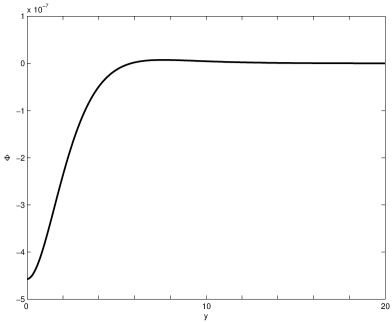
(a)

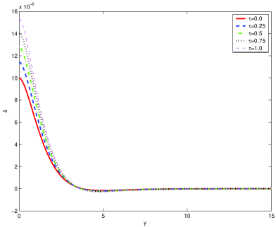
(b)

Figure 2: (a) The left panel shows a plot of the metric perturbation that results from the initial density inhomogeneity described in Eq. (44). (b) The right panel illustrates the time evolution of the corresponding density perturbation. The curves represent the spatial configuration of the density contrast at, from bottom to top, $\tau=0.0,\,0.25,\,0.5,\,0.75,\,1.0$

According to Eq. (26), once we know the metric perturbation we automatically know the time evolution of the density perturbation. The analytical expression for this is even longer than that for the metric perturbation so we will omit writing it down. Fig. 2(b) shows a plot of the density contrast for a selection of different times, thus illustrating how it grows with time.

Obtaining the relative temperature change $\Delta_{T}$ is now simply a matter of integrating Eq. (43) with the density contrast given by the analytical expression found above. Just as for the two perturbed quantities $\delta$ and $\Phi$, we demand that the $\Delta_{T}$ vanishes as $r\to\infty$. This allows us to write the relative temperature change as

$$\Delta_{T}(y,\tau)=- \frac{6mC}{k_{B}T_{00}}\left(\frac{L}{\eta_{0}}\right)^{2}(1+\tau)^{\frac{2}{3}}$$

$$\times\int_{\infty}^{y}\!dy^{\prime}\frac{1}{y^{\prime 2}}\int_{0}^{y^{\prime}}\!dy^{\prime\prime}y^{\prime\prime 2}\delta(y^{\prime\prime},\tau)\,.$$ (47)

The remaining constant which we need to determine in this expression is the initial temperature $T_{00}$. Since the initial time and amplitude of the density perturbation were chosen to correspond to perturbations in our own universe at the time of recombination, it is only natural that we also choose $T_{00}$ to be the temperature of the universe at the same time, namely $T_{00}=3\,000\,$K. Furthermore, the gas we consider consists of baryons, which allows us to use the mass $m=1.67\times 10^{-27}\,$kg. Using these values we find that the dimensionless constant that multiplies the integrals in Eq. (47) will be of the order $\sim 10^{7}$. Since the density contrast is of the order $\sim 10^{-5}$ we see that the relative change in temperature caused by the density perturbation must be very large. We can find a plot of this relative temperature change in Fig 3, which shows us that $\Delta_{T}$ is positive everywhere and that it grows with time. Thus, inserting the analytical expression for $\Delta_{T}$ into Eq. (42), we see that the entropy change induced by the density perturbation will be positive, and it will grow with time as the density inhomogeneity increases. This shows that the entropy of a gravitationally collapsing gas evolves according to the second law of thermodynamics up to first order. It is natural to assume that this will be the case to any order.

Strictly speaking, we have only showed this for the special initial density perturbation described in Eq. (44). In the appendix we show that this will be the case for all initial density perturbations of the class defined in the beginning of this section.

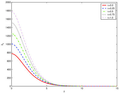
Figure 3: A plot of the temperature perturbation that corresponds to the density perturbation illustrated in Fig 2(b).

VI Conclusions

The main objective of this paper was to show that the entropy of an inhomogeneous gas increases as the gas collapses under the influence of gravity. Naively, one might expect the opposite to be the case since inhomogeneities in both the density and the temperature increase under such a collapse, which is an evolution that we generally associate with a decrease in entropy. By allowing for a transfer of energy from the gravitational potential to thermal energy, the temperature in the gas will increase as a result of the collapse. Treating the inhomogeneous gas as a first order perturbation to a homogeneous FRW model, we showed that the increase in temperature results in an increase in the entropy which outweighs any decrease due to increasing inhomogeneities in the temperature and and the density. This was shown to be the case for any initial density inhomogeneity which consists of one overdense region. Although our results were derived only up to first order in the inhomogeneity, it is only natural to extend the conclusions to any type of inhomogeneity. This allows us to conjecture that the entropy of a any gravitationally collapsing gas will always increase with time, in accordance with the second law of thermodynamics.

*

Appendix A More general perturbations

We define a class of perturbations where the initial profile has only one overdensity. The coordinate system is chosen so that the center of the overdensity is situated at the origin. Define the function

$$F(y,\tau)=\int_{0}^{y}\!dy^{\prime}y^{\prime 2}\delta(y^{\prime},\tau)\,.$$ (48)

From Eq. (31) we get that

$$\lim_{y\to\infty}F(y,\tau)=0\,.$$ (49)

The fact that the only overdensity is that at the origin implies that there exists a $y_{0}$ such that $\delta(y,\tau)>0$ for $0\leq y<y_{0}$ and $\delta(y,\tau)\leq 0$ for $y>y_{0}$. This along with Eq. (49) implies that $F(y,\tau)$ must be positive for all values of $y$,

$$F(y,\tau)>0\quad\mbox{ for }y>0\,.$$ (50)

The temperature change in Eq. (47) can be written as

$$\Delta_{T}(y,\tau)\propto-(1+\tau)^{2/3}\int_{\infty}^{y}\!dy^{\prime}\frac{F(y^{\prime},\tau)}{y^{\prime 2}}\,.$$ (51)

From this expression we see why the lower limit of the integration must indeed be $+\infty$: We require the temperature change to vanish at infinity. Since the integrand is always greater than zero, this can only be accomplished if the range of integration vanishes at infinity, which implies that the lower integration limit must be $+\infty$. This in turn implies that the integral in Eq. (51) will be negative for all $y$. Thus we have shown that $\Delta_{T}$ will be positive for all $y$. This is the first step in our proof. We must also show that $\Delta_{T}$ increases with time. In order to do this we differentiate Eq. (51) with respect to $\tau$. This yields the expression

$$\frac{\partial\Delta_{T}}{\partial\tau}\propto-\left(\frac{2}{3}(1+\tau)^{-1/3}\int_{\infty}^{y}\!dy^{\prime}\frac{F(y^{\prime},\tau)}{y^{\prime 2}}\right.$$

$$+\left.(1+\tau)^{2/3}\int_{\infty}^{y}\!\frac{dy^{\prime}}{y^{\prime 2}}\frac{\partial F(y^{\prime},\tau)}{\partial\tau}\right).$$ (52)

The first term inside the parentheses will be negative due to the same arguments as above. Using the definition in Eq. (48), we can write

$$H(y,\tau)\equiv\frac{\partial F(y,\tau)}{\partial\tau}=\int_{0}^{y}\!dy^{\prime}y^{\prime 2}\frac{\partial\delta(y^{\prime},\tau)}{\partial\tau}\,.$$ (53)

Again, using Eq. (49), we find that $\lim_{y\to\infty}H(y,\tau)=0$. We know that the effect of gravity on the density perturbation is such that overdense regions become more dense, while underdense regions become less dense. This means that $\frac{\partial\delta(y,\tau)}{\partial\tau}>0$ for $0\leq y<y_{0}$ and $\frac{\partial\delta(y,\tau)}{\partial\tau}\leq 0$ for $y>y_{0}$. Thus, just as for the integrand in Eq. (51), this implies that the integrand in Eq. (53) must be positive and hence that $H(y,\tau)$ must also be positive. The integral in the second term in Eq. (52) must therefore be negative since the integrand is positive while the integration path is negative. This proves that $\frac{\partial\Delta_{T}}{\partial\tau}$ is positive for all $y>0$ and $\tau>0$.

In summary, we have shown that a density perturbation of the class defined at the start of this appendix yields a temperature change $\Delta_{T}$ which is positive everywhere and grows with time. This concludes our proof.

References

- Spergel et al. (2003) D. Spergel et al., Astrophys. J. 148, 175 (2003), eprint astro-ph/0302209.
- Penrose (1977) R. Penrose, in Proceedings of the First Marcel Grossmann Meeting on General Relativity, edited by R. Ruffini (Elsevier North-Holland, 1977).
- Penrose (1979) R. Penrose, in General Relativity. An Einstein centenary survey, edited by S. Hawking and W. Israel (Cambrigde, 1979).
- Penrose (1981) R. Penrose, in Quantum gravity 2: A second Oxford symposium, edited by C. Isham, R. Penrose, and D. Sciama (Oxford: Clarendon Press, 1981).
- Kittel and Kroemer (1980) C. Kittel and H. Kroemer, Thermal Physics (W.H. Freeman, 1980), 2nd ed.
- Mukhanov et al. (1992) V. Mukhanov, H. Feldman, and R. Brandenberger, Phys.Rep. 215 (1992).
- Ma and Bertschinger (1995) C.-P. Ma and E. Bertschinger, Ap.J 455, 7 (1995), eprint astro-ph/9506072.
- Brandenberger (2004) R. Brandenberger, Lect.Notes Phys 646, 127 (2004), eprint hep-th/0306071.
- Davies (1974) P. Davies, The Physics of Time Asymmetry (Surrey University Press, 1974).
- Misner et al. (1973) C. Misner, K. Thorne, and J. Wheeler, Gravitation (Freeman, 1973).
- Carroll and Ostlie (1996) B. Carroll and D. Ostlie, Modern Astrophysics (Addison-Wesley, 1996).