CPT Violation and Decoherence in Quantum Gravity

In these lectures I review, in as much pedagogical way as possible, various theoretical ideas and motivation for violation of CPT invariance in some models of Quantum Gravity, and discuss the relevant phenomenology. Since the subject is vast, I pay particular emphasis on the CPT Violating decoherence scenario for quantum gravity, due to space-time foam. In my opinion this seems to be the most likely scenario to be realised in Nature, should quantum gravity be responsible for the violation of this symmetry. In this context, I also discuss how the CPT Violating decoherence scenario can explain experimental “anomalies” in neutrino data, such as LSND results, in agreement with the rest of the presently available data, without enlarging the neutrino sector.

1 Introduction and Summary

Next year, Special Relativity celebrates a century of enormous success, having passed many stringent experimental tests, in both its classical and quantum versions (relativistic quantum field theories in flat space times). Unfortunately, the same is not true for its curved-space counterpart, General Relativity. A consistently quantized theory of gravity, that is a dynamical theory of curved geometries themselves, still remains a mystery. Despite the enormous effort invested for this purpose on behalf of the scientic community over the past ninety years, Quantum Gravity is still far from being understood as a physical theory.

Of course, elegant and mathematically consistent models, such as string or, better, brane theorystrings , have been developed to a great detail from a mathematical viewpoint. Nevertheless there are still many fundamental issues and questions which remain unresolved. For instance, the complete process of evaporation of a black hole, or the inverse process of collapsing matter to form a Black Hole, are not completely understood in string theory. The counting of microstates and verification of the Hawking-Bekenstein entropy/area law have been understood mathematically only in specific cases of extremal black holes, and probably this is the only case that can be studied rigorously in such a framework. Other issues, like the possible existence of space-time foam, that is microscopic singular fluctuations of the (quantum) geometry, which give the space time a “foamy”, topologically non trivial and possibly non-continuous structure at Planck scales ($10^{-35}$ m), still remain far from being resolved in the context of string theory.

In emntheory it was suggested that a consistent mathematical framework for dealing with such issues in the context of string theory was the Liouville non-critical srting theory approach, involving strings propagating in non-conformal space-time backgrounds. This violation of conformal symmetry, which lies at the cornerstone of critical string theory, is remedied by the non-decoupling of the Liouville mode, which enters as a whole new target space dimension. In certain models of stringy foam, this extra dimension has time-like signature, and hence it can be identified with a target time, thereby giving the time coordinate a fundamentally irreversible nature, as a result of specific properties of the Liouville dynamics. Indeed, the latter acts as a local renormalization-group scale on the world-sheet of the string, and as such is irreversible. This fundamental irreversibility of non-critical string theory makes it analogous to non-equilibrium systems in field theory. From this point of view, then, critical strings are viewed as asymptotic “equilibrium points” in string theory space.

Alternative approaches to Quantum Gravity, on the other hand, such as the loop gravity approach loop , which has the ambition of formulating a space-time background independent quantum theory of Gravity, have only relatively recently began to deal with non-flat space times (such as those with cosmological constant) or highly curved ones (black holes etc.), and hence their full potential in dealing with the above issues is still not exploredsmolin . These are very elegant theories from a geometrical viewpoint, which are based on the analogy of gravity to non Abelian gauge theories. Understanding the rôle of matter in such gravity theories is a pressing task, in order to give such mdoels phenomenological relevance. In addition to loop gravity, non commutative geometrylukierski ; glikman is another mathematically elegant route that would certainly prove to be relevant for a dynamical quantum theory of space time at Planck scales, where space time may be discrete. This approach, although existing for some time, has only recently started to be paid attention by the bulk of the theoretical physicists, with a plethora of applications, ranging from field theoretic models to string and brane theories.

A theoretical model, however, no matter how detailed and elegant it might be, does not become a physical theory unless it makes some form of contact with experiment. Thus, to understand and be guided in our quest for quantum gravity we need experimentally testable or falsifiable predictions. Critical strings, or other approaches to quantum gravity, which respect all local symmetries of classical General Relativity, did not make any predictions for low-energy theories which could be testable in the foreseeable future. The reason is simple: the coupling constant of gravity, the Newton constant $G_{N}\propto 1/M_{P}^{2}$ (in four dimensions) is very small, and, on account of local Lorentz symmetry and general covariance, quantities of possible experimental interest, such as cross sections and probabilities, would be characterised by quantum gravitational loop corrections which would be proportional to some power of curvature tensors. The latter having dimensions of momentum squared, would imply that such quantities would be suppressed at least by the inverse square (and most likely by higher powers) of the Planck Mass scale. This would make the prospects for detection of such quantum gravity effects difficult, if not impossible, for the foreseeable future. Of course this does not necessarily mean that such approaches are physically incorrect, what it means is that, even if they represent reality, we would have no way of testing them in the foreseeable future, and as such they would remain solely mathematically consistent models.

On the other hand, recently, more and more physicists contemplate the idea that some of the fundamental symmetries or laws that govern classical General and Special Relativity, such as linear Lorentz symmetry, or principles such as the equivalence principle, may not be valid in a full quantum theory of gravity. If true, then, this would probably imply that the above-mentioned Planck-mass strong suppression factors could be modified in such a way that quantum gravity effects are enhanced, thereby leading to some testable/falsifiable predictions in the near future. For instance, in the non-critical string approach to quantum gravity advocated in emntheory , deviation from conformal invariance due to peculiar backgrounds in string theory, including foamy ones, imply in some models at an effective low-energy field theory level, modified dispersion relations for photons or at most for some electrically neutral gauge bosons. Such modifications dot not occur not for charged probes or in general chiral mattersynchro , thereby violating a form of the equivalence principle, in the sense of the non-universality of gravity effects. In such models it is a gauge symmetry that protects the dispersion relation of charged or chiral matter probes, which, unlike photons, do not interact with space time defects in the foam, the latter consisting of point-like branes in string theoryhorizons . The modification to the dispersion relations due to such quantum gravity effects are suppressed only by a single power of Planck Massaemn . Such minimal suppression models for photons are not far from being tested, for instance by future Gamma Ray Burst astronomyemnnature ; grb . On the other hand, models of quantum gravity foam with universal modified dispersions linearly suppressed by the Planck Mass scale are already excluded by means of astrophysical observations of Synchrotron radiation from Crab Nebulacrab ; jacobpoland , and one is not far from reaching sensitivities quadratic to inverse Planck masssynchro .

In this context, interesting “bottom-up” approaches to quantum gravity have been proposed and developed rigorously, such as the Doubly-Special Relativity (DSR) theories nlls , which are at the focus of this meeting. According to such approaches, the conventional Lorentz symmetry of flat Minkowski space time is not valid, but instead one has a symmetry under non-linear extensions of the Lorentz transformations. Such non-linear extensions are not unique, and this poses an interesting theoretical challenge for these models. The basic idea behind such theories is that the Planck scale should be observer independent, and hence such non-linear models are characterised not only by the invariance under frame changes of the dimensionless speed of light in vacuo, but also by the frame-invariance of a dimensionful length scale, the Planck length. For this reason, although at present formulated in flat space times, such non-linear extensions of Lorentz symmetry are viewed as a prelude to more complete models of quantum gravity, where the local group is not the conventional (linear) Lorentz, thereby violating the strong form of the equivalence principle. However it remains to be proven whether such models are viable as candidates for a complete and realistic theory of quantum gravity. In other lectures in this meeting we shall hear more about the mathematical foundations and properties of such theories amelino , and their phenomenology grillo ; jacobpoland ; piran , where we refer the reader for details.

In all approaches mentioned so far as candidate theories for quantum gravity there is a common feature, associated with the violation of a theorem whose validity characterises all consistent flat-space time relativistic quantum field theories known to date. This is the CPT theorem pauli ; bell ; jost ; wight . The violation of this (discrete) space-time symmetry may have important phenomenological implications for low energy physics, and indeed one is prompted immediately to think that this may be a way of testing or falsifying experimentally various theoretical models of quantum gravity entailing such a violation.

There is a number of fundamental questions, however, that one has to ask before embarking on a study of the phenomenology of CPT Violation: (i) What are the theories which allow for CPT breaking?, (ii) How (un)likely is it that somebody, someday finds CPT Violation in the Laboratory, and why?, (iii) What formalism does one has to adopt? Indeed, since our current phenomenology of particle physics is based on CPT invariance, how can we be sure of observing CPT Violation and not something else? And finally, (iv) there does not seem to be a single “figure of merit” for CPT violation. Then how should we compare various “figures of merit” of CPT tests (e.g. direct mass measurement between matter and antimatter (e.g. $K^{0}$-${\overline{K}}^{0}$ mass difference a la CPLEAR), quantum decoherence effects, modifications to Einstein-Podolsky-Rosen (EPR) states in meson factories, neutrino mixing, electron g-2 and cyclotron frequency comparison, neutrino spin-flavour conversion etc.)

In some of these questions I shall try to give answers in the context of the present set of Lectures. I shall not try to present a complete overview of phenomenological tests of CPT Invariance, however, because the subject is vast, and already occupies a considerable part of the published literature. In these lectures I will place the emphasis on neutrino tests of CPT invariance, because as I will argue below, in many instances neutrinos seem to provide at present the best bounds on possible CPT violation. However, I must stress that, precisely because CPT violation is a highly model dependent feature of some approaches to quantum gravity (QG), there may be models in which the sensitivity of other experiments on CPT violation, such as astrophysical experiments, is superior to that of current neutrino experiments. For this reason I will also give a brief outline of alternative tests of CPT violation.

My lectures will focus on the following three major issues:

(a) What is CPT Symmetry: I will give a definition of what we mean by CPT invariance, and under what conditions this invariance holds.

(b) Wny CPT Violation ?: Currently there are various Quantum Gravity Models which may violate Lorentz symmetry and/or quantum coherence (unitarity etc), and through this CPT symmetry: (i) space-time foam foam (local field theories garay , non-critical strings emntheory etc.), (ii) (non supersymmetric) string-inspired standard model extension with Lorentz Violation kostel , (iii) Loop Quantum Gravity loop . (iv) CPT violation may also occur at a global scale, cosmologically cosmonem , as a result of a cosmological constant in the Universe, whose presence may jeopardize the definition of a standard scattering matrix.

(c) How can we detect CPT Violation? : Here is a current list of most sensitive particle physics probes for CPT tests: (i) Neutral Mesons: Kaons ehns ; emn , B-mesons, and their entangled states in $\phi$ and $B$ factories huet ; benatti1 ; bernabeu .

(ii) anti-matter factories: antihydrogen antihydro (precision spectroscopic tests on free and trapped molecules kostel ; bluhm ; mavroyoko ),

(iii) Low energy atomic physics experiments bluhm , including ultra cold neutron experiments in the gravitational field of the Earth.

(iv) Astrophysical Tests (especially Lorentz-Invariance violation tests, via modified dispersion relations of matter probes etc.) emnnature ; grb

(iv) Neutrino Physics, on which we shall mainly concentrate in these lectures mavrovenice .

I shall be brief in my description due to space restrictions. For more details I refer the interested reader to the relevant literature. I will present some elementary proofs of theorems that will be essential for the formalism of CPT Violation and its phenomenology. I will not be complete in reviewing the phenomenology of CPT violation; in my lectures I will place emphasis on a specific type of violation, that through quantum decoherence, which I believe to be the most likely one to charactrise space-time foam theories of quantum gravity; this belief is based on the fact that decoherence may be compatible with fundamental local symmetries of space time, such as Lorentz invariance mill ; discr . For completeness, however, I will also give a brief exposition of alternative ways of CPT violation, and refer the reader to some key references, where more detailed information is provided on those topics. Needless to say that I am fully aware of the vastness of the topic of CPT Violation, which grew enormously in recent years, and I realize that I might not have done a perfect job here; I should therefore apologize beforehand for possible omissions in references, and topics, but this was not intentional. I do hope, however, that I give here a rather satisfactory representation of the current situation regarding this important research topic.

2 Theoretical Motivation for CPT Violation and Formalism

2.1 The CPT theorem and how it may be evaded

The CPT theorem refers to quantum field theoretic models of particle physics, and ensures their invariance under the successive operation (in any order) of the following discrete transformations: C(harge), P(arity=reflection), and T(ime reversal). The invariance of the Lagrangian density ${\cal L}(x)$ of the field theory under the combined action of CPT is a property of any quantum field theory in a Flat space time which respects: (i) Locality, (ii) Unitarity and (iii) Lorentz Symmetry.

$$\Theta{\cal L}(x)\Theta^{\dagger}={\cal L}(-x)~{},~{}\Theta=CPT~{},~{}{\cal L}={\cal L}^{\dagger}$$ (1)

The theorem has been suggested first by Lüders and Pauli pauli , and also by John Bell bell , and has been put on an axiomatic form, using Wightman axiomatic approach to relativistic (Lorentz invariant) field theory, by Jost jost . Recently the Lorentz covariance of the Wightmann (correlation) functions of field theories wight as an essential requirement for a proof of CPT has been re-emphasized in greenb , in a concise simplified exposition of the work of Jost. The important point to notice in that proof is the use of flat-space Lorentz covariance, which allows the passage onto a momentum (Fourier) formalism. Basically, the Fourier formalism employs appropriately superimposed plane wave solutions for fields, with four-momentum $p_{\mu}$. The proof of CPT, then, follows by the Lorentz covariance transformation properties of the Wightman functions, and the unitarity of the Lorentz transformations of the various fields.

In curved space times, especially highly curved ones with space-time boundaries, such as space-times in the (exterior) vicinity of black holes, where the boundary is provided by the black hole horizons, or space-time foamy situations, in which one has vacuum creation of microscopic (of Planckian size $\ell_{P}=10^{-35}$ m) black-hole horizons foam , such an approach is invalid, and Lorentz invariance, and possibly unitarity, are lost. Hence, such models of quantum gravity violate requirements (ii) & (iii) of the CPT theorem, and hence one should expect its violation.

It is worthy of discussing briefly the basic mechanism by which unitarity may be lost in space-time foamy situations in quantum gravity. This is the lecturer’s favorite route for possible quantum-gravity induced CPT Violation, which may hold independently of possible Lorentz invariance violations. It is at the core of the induced decoherence by quantum gravity ehns ; emn .

The important point to notice is that, in general, space-time may be discrete and topologically non-trivial at Planck scales $10^{-35}~{}m$, which might (but this is not necessarymill ; discr ), imply Lorentz symmetry Violation (LV), and hence CPT Violation (CPTV). Phenomenologically, at a macroscopic level, such LV may lead to extensions of the standard model which violate both Lorentz and CPT invariance kostel .

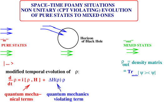
Figure 1: A basic mechanism for loss of information in a space time foamy situation.

In addition, there may be an environment of gravitational degrees of freedom (d.o.f.) inaccessible to low-energy experiments (for example non-propagating d.o.f., for which ordinary scattering is not well defined emn ). This will lead in general to an apparent information loss for low-energy observers, who by definition can measure only propagating low-energy d.o.f. by means of scattering experiments. As a consequence, an apparent lack of unitarity and hence CPTV may arise, which is in principle independent of any LV effects. The loss of information may be understood simply by the mechanism illustrated in fig. 1. In a foamy space time there is an ongoing creation and annihilation of Quantum Gravity singular fluctuations (e.g. microscopic (Planck size) black holes etc), which indeed implies that the observable space time is an open system. When matter particles pass by such fluctuations (whose life time is Planckian, of order $10^{-43}$ s), part of the particle’s quantum numbers “fall into” the horizons, and are captured by them as the microscopic horizon disappears into the foamy vacuum. This may imply the exchange of information between the observable world and the gravitational “environment” consisting of degrees of freedom inaccessible to low energy scattering experiments, such as back reaction of the absorbed matter onto the space time, recoil of the microscopic black hole etc.. In turn, such a loss of information will imply evolution of initially pure quantum-mechanical states to mixed ones for an asymptotic observer.

As a result, the asymptotic observer will have to use density matrices instead of pure states: $\rho_{out}={\rm Tr}_{\rm unobs}|out><out|=$ $ $\rho_{in}\$\neq SS^{\dagger}$, with $S=e^{iHt}$ the ordinary scattering materix. Hence, in a foamy situation the concept of the scattering matrix is replaced by that of the superscattering matrix, $, introduced by Hawking foam , which is a linear, but non-invertible map between “in” and “out” density matrices; in this way, it quantifies the unitarity loss in the effective low-energy theory. The latter violates CPT due to a mathematical theorem by R.Wald, which we describe in the next subsection wald .

Notice that this is an effective violation, and indeed the complete theory of quantum gravity (which though is still unknown) may respect some form of CPT invariance. However, from a phenomenological point of view, this effective low-energy violation of CPT is the kind of violation we are interested in here. A word of caution is necessary at this point. Some theorists believe that quantum gravity does not entail an evolution of a pure quantum state to a mixed one, but, as is the case in some quantum mechanical decoherence models of open systems, to be discussed below, the purity of states is maintained during the quantum-gravity induced decoherent evolution. If this is the case, then CPT may be conserved in such models, provided, of course, Lorentz invariance and locality of interactions are respected.

2.2 $ matrix and strong CPT Violation (CPTV)

The theorem of R. Wald states the following wald : if $ $\neq S~{}S^{\dagger}$, then CPT is violated, at least in its strong form, in the sense that the CPT operator is not well defined.

For instructive purposes we shall give here an elementary proof. Suppose that CPT is conserved, then there exists a unitary, invertible CPT operator $\Theta$: $\Theta{\overline{\rho}}_{in}=\rho_{out}.$ Since the density matrix acts on a tensor product space between ket and bra vectors by definition, $\rho=\psi\otimes{\overline{\psi}}$, the action of $\Theta$ is defined schematically as: $\Theta=\theta\theta^{\dagger}$, with $\theta$ acting on state vectors $\psi$, and being anti-unitary, i.e. $\theta^{\dagger}=-\theta^{-1}$.

Asuming that such a $\Theta$ exists, we have: $\rho_{out}=$ $ $\rho_{in}\rightarrow\Theta{\overline{\rho}}_{in}=$$ $\Theta^{-1}{\overline{\rho}}_{out}\rightarrow$ ${\overline{\rho}}_{in}=\Theta^{-1}$$ $\Theta^{-1}{\overline{\rho}}_{out}$.

But ${\overline{\rho}}_{out}=$$${\overline{\rho}}_{in}$, hence :

$${\overline{\rho}}_{in}=\Theta^{-1}\$\Theta^{-1}\${\overline{\rho}}_{in}.$$ (2)

The last relation implies that $ has an inverse

$$\$^{-1}=\Theta^{-1}\$\Theta^{-1},$$ (3)

which, however, as we explain now is impossible, due to the information loss in case a pure state evolves into a mixed one.

To provewald this last statement formally we first notice that from (3) one also obtains the relation:

$$\Theta=\$\Theta^{-1}\$.$$ (4)

Consider now a pure state density matrix $\rho_{in}=|IN\rangle\langle IN|$, which evolves to the density matrix (mixed state) $$\rho_{in}$. As a result of (4), the mixed state $\Theta^{-1}$$$\rho_{in}$ must evolve to the pure state $\Theta\rho_{in}$. However, suppose we have an out state $\psi$, which we obtain by the action of $ on an IN density matrix $\sigma$, that is:

$$\$\sigma=\psi\otimes{\overline{\psi}}$$ (5)

where, as mentioned above, $\otimes$ denotes the appropriate tensor product of Hilbert spaces spanned by ket and bra vectors. One may expand $\sigma$ in terms of its eigenvectors $\phi_{i}$, corresponding physically to a weighted superposition of states that comprise the mixed state $\sigma$:

$$\sigma=\sum_{i}p_{i}\phi_{i}\otimes{\overline{\phi}}_{i},$$ (6)

with $p_{i}$ positive, and $\sum_{i}p_{i}=1$. Since by definition $ is a linear map, we have:

$$\sum_{i}p_{i}\$(\phi_{i}\otimes{\overline{\phi}}_{i})=\psi\otimes{\overline{\psi}}$$ (7)

Consider now an OUT state vector $\chi$ orthogonal to $\psi$. Taking the expectation value of (7) in the state $\chi$ we obtain:

$$\sum_{i}p_{i}\langle\chi|\$(\phi_{i}\otimes{\overline{\phi}}_{i})|\chi\rangle=0$$ (8)

Each term in (8) is non negative, due to the positive-definiteness of $p_{i}$ and the positivity of the density matrix (by definition) $\$(\phi_{i}\otimes{\overline{\phi}}_{i})$. Therefore, (8) implies

$$\langle\chi|\$(\phi_{i}\otimes{\overline{\phi}}_{i})|\chi\rangle=0$$ (9)

for all $i$ and all $\chi$ orthogonal to $\psi$. This implies

$$\$(\phi_{i}\otimes{\overline{\phi}}_{i})=\psi\otimes{\overline{\psi}}$$ (10)

for all $i$, i.e. each initial pure state $\phi_{i}$ must evolve to the same final pure state $\psi$. In that case, $\theta^{-1}\psi$ must evolve to the final state $\theta\phi_{i}$ for all $i$. This is impossible if there is more than one $\phi_{i}$, i.e. if the density matrix $\sigma$ represents a mixed state.

Hence, in case where decoherence implies the evolution of a pure state to a mixed one, CPT must be violated, at least in its strong form, in the sense of $\Theta$ not being a well-defined operator, and the non existence of the inverse of $, as discussed previoulsy. The non invertibility of $ should not be considered as a surprise in that case, as a result of the involved loss of information in the problem. CPT symmetry, and also by the same arguments microscopic time reversalwald , fail in a dramatic way in such a case: microscopic time-reversed dynamics does not merely fail to be the same as time evolution forward in time, which would simply mean the non commutativity of the corresponding operators/generators of the symmetry with the hamiltonian of the system under consideration, but does not exist at all.

As I remarked before, this is my preferred way of CPTV by Quantum Gravity, given that it may occur in general independently of LV and thus preferred frame approaches to quantum gravity. Indeed, I should stress at this point that the above-mentioned gravitational-environment induced decoherence may be Lorentz invariant mill , the appropriate Lorentz transformations being slightly modified to account, for instance, for the discreteness of space time at Planck length discr . This is an interesting topic for research, and it is by no means complete. Although the lack of an invertible scattering matrix in most of these cases implies a strong violation of CPT, nevertheless, it is interesting to demonstrate explicitly whether some form of CPT invariance holds in such cases waldron . This also includes cases with non-linear modifications of Lorentz symmetry nlls , discussed in this School, which arise from the requirement of viewing the Planck length as an invariant (observer-independent) proper length in space time.

It should be stressed at this stage that, if the CPT operator is not well defined, then this may lead to a whole new perspective of dealing with precision tests in meson factories. In the usual LV case of CPTV kostel , the CPT breaking is due to the fact that the CPT operator, which is well-defined as a quantum mechanical operator in this case, does not commute with the effective low-energy Hamiltonian of the matter system. This leads to mass differences between particles and antiparticles. If, however, the CPT operator is not well defined, as is the case of the quantum-gravity induced decoherence ehns ; emn , then, the concept of the ‘antiparticle’ gets modified bernabeu . In particular, the antiparticle space is viewed as an independent subspace of the state space of the system, implying that, in the case of neutral mesons, for instance, the anti-neutral meson should not be treated as an identical particle with the corresponding meson. This leads to the possibility of novel effects associated with CPTV as regards entangled states of Einstein-Podolsky-Rosen (EPR) type, which may be testable at meson factories bernabeu . We shall discuss this in some detail later on.

2.3 CPT Symmetry without CPT Symmetry?

An important issue which arises at this point is whether the above violation of CPT symmetry is actually detectable experimentally. This issue has been examined in wald , where it was proposed that despite the strong CPT violation in cases where decoherence leads to an evolution of a pure state to a mixed one, there is the possibility for a softer (weaker) form of CPT invariance in such cases, compatible with the non-invertibility of $.

The main idea behind such a weak form of CPT invariance is that, although in the full theory CPT is violated in the above sense, nevertheless one can still define asymptotic pure scattering IN and OUT states as the CPT inverse of each other. In formal terms, although in the full theory $\Theta$ is not well defined, however one can define pure states $\psi\in{\cal H}_{IN}$, and $\phi\in{\cal H}_{OUT}$ in the respective Hilbert spaces ${\cal H}$ of IN and OUT states, such that the following equality between probabilities ${\cal P}$ holds:

$${\cal P}(\psi\rightarrow\phi)={\cal P}(\theta^{-1}\phi\rightarrow\theta\psi)$$ (11)

If only pobabilities are measured experimentally, which is certainly our experience so far, then the equality (11) would imply that the strong form of CPT invariance would be undetectable experimentally.

From the point of view of the superscattering matrix $, the equality (11) implies the following relationwald :

$$\langle\phi|\$(\psi\otimes{\overline{\psi}})|\phi\rangle=\langle\theta\psi|\$(\theta^{-1}\phi\otimes{\overline{\theta}^{-1}\phi})|\theta\psi\rangle$$ (12)

or, equivalently :

$$\$^{\dagger}=\Theta^{-1}\$\Theta^{-1}$$ (13)

when the action is considered on pure asymptotic states. Relation (13) is compatible with the non-existence of an inverse of $, unless the full CPT invariance holds, which would imply unitarity of $, i.e. $^† = $^-1. Wald has argued in favour of this conclusion by considering a simple case of finite-dimension ($n$) Hilbert spaces of IN and OUT states, and assuming that every pure IN state evolves to the density matrix $1/n\delta^{a}_{b}$ in the OUT Hilbert space. It is clear that in this example $^-1 does not exist, but for all $\psi$ and $\phi$ the relation (11) holds, since both sides equal $1/n$.

2.4 Decoherence and Purity of States under Evolution

Since the above result of weak CPT invariance requires the purity of asymptotic scattering states, a natural question to ask is whether there exist concrete models of decoherence where the purity of an initial state vector remains, while time irreversibility holds.

A physically acceptable framework for discussing decohering evolution of an open quantum mechanical system is that of Lindblad or the so-called dynamical semigroup approachlindblad , which ensures the complete positivity of the density matrix $\rho(t)$ at any time moment $t$ during the evolution, and the conservation of probability ${\rm Tr}\rho=1$. The Lindblad evolution of open systemslindblad , with Hamiltonian $H$, interacting with an environment through operators $D_{j},D^{\dagger}_{j}$, is described as a linear evolution in the density matrix $\rho$:

$${\dot{\rho}}=i[\rho,H]+{\cal D}[\rho];\qquad{\cal D}[\rho]=\sum_{j}\left(\{\rho,D_{j}^{\dagger}D_{j}\}-2D_{j}\rho D_{j}^{\dagger}\right)$$ (14)

where $\{.,.\}$ denotes an anticommutator. The Hamiltonian $H$ in (14) may contain terms from the environmental entanglement which can be expressed as commutators with $\rho$, and hence it should be understood as an effective Hamiltonian of the system. The decoherence term ${\cal D}[\rho]$, on the other hand, cannot be expressed as such a commutator.

To ensure energy conservation on the average, and monotonic increase of the von-Neumann entropy $S=-{\rm Tr}\left(\rho{\rm ln}\rho\right)$, one has to impose self-adjointness of the Lindblad environmental operators

$$D_{j}^{\dagger}=D_{j}$$ (15)

and also require that these operators commute with the Hamiltonian

$$[D_{j},H]\qquad{\rm for}\quad{\rm all}\quad j$$ (16)

This leads to a double commutator structure of the decoherence terms in (14):

$${\cal D}[\rho]=\sum_{j}[D_{j},[D_{j},\rho]]$$ (17)

In general, in this type of decoherence one has the evolution of a pure state into a mixed one. However, there exist subclasses of Lindblad evolution, in particular energy-driven simple decoherence modelshoughston ; adler , where the purity of state vectors is preserved. A mathematical criterion for this feature is that

$$\rho^{2}=\rho,\qquad{\rm Tr}\rho=1,$$ (18)

during the evolution.

In such models, $D_{j}=\lambda_{j}H$, with $\lambda_{j}$ c-number constants. Without loss of generality, we can substitute in such a case the sums in (17) by a single environmental operator

$$D=\lambda H,\qquad\lambda^{2}=\sum_{j}\lambda_{j}^{2}$$ (19)

This simplifies the situation and will suffice for our purposes in this work.

In this type of decoherence, the density matrix evolution preserves the purity of states, and can be written in terms of stochastic Ito differential equations for the state vectors $|\psi\rangle$ (or equivalently the pure state density matrix $\rho=|\psi\rangle\langle\psi|$):

$$d\rho=-i[H,\rho]dt-\frac{1}{8}[D,[D,\rho]]dt+\frac{1}{2}[\rho,[\rho,D]]dW_{t}$$ (20)

where $t$ is the time, and $dW_{t}$ is an Ito stochastic differential obeying

$$dW_{t}^{2}=dt,\qquad dtdW_{t}=0$$ (21)

which are the equivalent of white noise conditions. Needelss to say that one can generalise the above equation to the case where sums of $D_{j}$ operators are involved, but as we mentioned above this will not be necessary for our purposes here.

We remark that, in terms of state vectors $|\psi\rangle$, the first term in (20) is nothing but the Schrödinger Hamiltonian term $-iH|\psi\rangle$, while the second term resembles Fokker-Planck stochastic diffusion terms. Unlike the Schrödinger term, the diffusion term is not invariant under the time reversal operation $t\rightarrow-t$ and $i\rightarrow-i$, and hence time irreversibility occurs in the problem, despite the purity of states.

Upon using (19) in (20), one obtains a stochastic equation for this energy-driven decoherence:

$$d\rho=-i[H,\rho]-\frac{\lambda^{2}}{8}[H,[H,\rho]]dt+\frac{\lambda}{2}[\rho,[\rho,H]]dW_{t}$$ (22)

The double commutator of the Hamiltonian, together with the purity-of-states condition (18), leads to the following order of the decoherence term in such models, obtained by considering the vacuum expectation value of the double commutator term in (22): $\gamma\equiv\langle\langle{\cal D}[\rho]\rangle\rangle={\rm Tr}\left(\rho\frac{\lambda^{2}}{8}[H,[H,\rho]]\right)$. Using as a complete orthonormal basis of states energy eigenstates $|m\rangle$, then, it is straightforward to see that the above estimate leads to the square of the energy variance

$$\gamma=\frac{\lambda^{2}}{8}\left(\Delta H\right)^{2}=\langle\langle H^{2}\rangle\rangle-\left(\langle\langle H\rangle\rangle\right)^{2}$$ (23)

for this model of decoherence.

In quantum-gravity driven models of decoherence it is natural to assume that $\lambda^{2}\propto 1/M_{P}$, where $M_{P}\sim 10^{19}$ GeV is the Planck scale, which is expected to be the characteristic scale of quantum gravity. In such models then one obtains the following estimate for the decoherence coefficient $\gamma$adler

$$\gamma\sim\left(\Delta H\right)^{2}/M_{P}$$ (24)

We shall come back to physical applications of this case later on, when we discuss sensitive probes of quantum mechanics, such as neutral mesons and neutrinos.

Before closing this subsection we should remark that other types of decoherence models, which are not energy driven, but correspond to spontaneous localisation in space, also exist. One such model is the one presented in ghirardi , in which the operator $D$ is taken to be proportional to the spatial coordinate operator $q$, thereby leading to spatial localisation. In such a case again the decoherence coefficient $\gamma$ (24) is found to be proportional to the square of the position operator variance $\gamma\propto\left(\Delta q\right)^{2}$, expressing, e.g. spatial separation between centres of wavepackets, resulting for instance from the mass difference.

2.5 More General Case: Dynamical Semi-Group Approach to Decoherence, and Evolution of Pure States to Mixed

In the previous subsection we examined special cases of Lindblad decohering evolution, which preserved the purity of quantum states. The Lindblad approach to decoherence, however, in general has the feature of implying an evolution of a pure state to a mixed one, in the sense of ${\rm Tr}\rho(t)^{2}\neq{\rm Tr}\rho(t)$, thereby leading to a violation of the strong form of CPT, according to the theorem of wald . The general Lindblad evolution can be formulated in such a way that no detailed knowledge of the underlying microscopic dynamics of the decohering environment is necessary in order to arrive at certain conclusions of phenomenological interest. This is achieved by means of the so-called dynamical semigroups approach to decoherence lindblad , which is a generic formalism to describe a decohering evolution obeying some basic properties. The time irreversibility in this approach is linked to the lack of an inverse of an element in an appropriate semigroup.

Consider the generic case of a decohering (of Lindblad, or even more general, type) evolution for an $N$-level system, that is a system whose Hamiltonian (energy) eigenstates span an $N$-dimensional state vector space. The decohering operators, assumed bounded for our purposes here, can be represented by $N\times N$ matrices generated by a basis $F_{\mu},~{}\mu=0,1,\dots N^{2}-1$, endowed by the scalar product $(F_{\mu},F_{\nu})=\frac{1}{2}\delta_{\mu\nu}$. For the purposes in this work we shall be dealing explicitly with $N=2,3$ level systems, in which cases the basis $\{F_{\mu}\}$ consists of: (i) the three $2\times 2$ Pauli matrices plus the $2\times 2$ identity matrix $I_{2}$ for the $N=2$ case, and (ii) the $3\times 3$ Gell-Mann matrices $\Lambda_{i}$,$i=1,\dots 8$ plus the $3\times 3$ identity matrix $I_{3}$ for the $N=3$ case.

Generically the matrices $F_{\mu}$ satisfy the following commutation relations:

$$[F_{i},F_{j}]=i\sum_{k}f_{ijk}F_{k},\qquad 1\leq i,j,k\leq 8$$ (25)

where $f_{ijk}$ are the structure constants of the $SU(N)$ group, and we follow the notation that Latin indices run from 1, to $N^{2}-1$, while Greek indices run from $0,1,\dots N^{2}-1$.

Expanding the environmental operators, as well as the (effective) Hamiltonian and the density matrix in (14) in terms of the basis $\{F_{\mu}\}$:

$$H=\sum_{\mu}h_{\mu}F_{\mu},\qquad\rho=\sum_{\mu}\rho_{\mu}F_{\mu},\qquad D_{j}=\sum_{mu}d^{(j)}_{\mu}F_{\mu}$$ (26)

and imposing the hermiticity of $D$, which ensures the monotonic increase of the von Neumann entropy $S=-{\rm Tr}\rho{\rm ln}\rho$, we can write the decoherence term ${\cal D}[\rho]$ in (14) as:

$${\cal D}[\rho]_{\rm Lindblad}=\sum_{\mu,\nu}L_{\mu\nu}\rho_{\mu}F_{\nu},$$ (27)

where the matrix $L_{\mu\nu}$ is real and symmetric, with the properties:

$$L_{\mu 0}=L_{0\mu}=0,\qquad L_{ij}=\frac{1}{2}\sum_{k,l,m}({\vec{d}}_{m}\cdot{\vec{d}}_{k})f_{iml}f_{ikj},$$ (28)

whereby ${\vec{d}}_{\mu}=(d_{\mu}^{(1)},\dots d_{\mu}^{(N^{2}-1)})$.

The vanishing of the first row and column is due to entropy increase. Notice that if we do not impose the requirement of energy conservation on the average, then it is not necessary to assume the commutativity of the operators with the Hamiltonian, so in general $[D_{j},H]\neq 0$. In fact below we shall examine some examples where energy may be violated due to foam interactions.

The evolution equation (14), then, reads:

$${\dot{\rho}}=\sum_{i,j}h_{i}\rho_{j}f_{ij\mu}+\sum_{\nu}L_{\mu\nu}\rho_{\nu},\qquad\mu,\nu=0,\dots N^{2}-1.$$ (29)

where the overdot denotes derivative with respect to time $t$.

Probability conservation ${\rm Tr}\rho(t)=1$ at any time moment $t$ implies that the differential equation for the $\rho_{0}$ component decouples, yielding

$$\rho_{0}(t)={\rm const}$$ (30)

The remaining differential equations (29) then can be written in the form:

$${\dot{\rho}}_{k}=\sum_{j}\left(\sum_{i}h_{i}f_{ijk}+L_{kj}\right)\rho_{j}=\sum_{k}{\cal M}_{kj}\rho_{j}$$ (31)

Representing by ${\cal A}$ the matrix that diagonalises the matrix ${\cal M}$, and letting $\{\lambda_{1},\dots\lambda_{N^{2}-1}\}$ be the set of eigenavalues of ${\cal M}$, and $\{v_{1},\dots v_{N^{2}-1}\}$ be the corresponding set of its eigenvectors, we have for the $ij$ elements of ${\cal A}$: ${\cal A}_{ij}=(v_{i})_{j}$. The solution of (31), then, can be written as:

$$\rho_{i}(t)=\sum_{k,j}e^{\lambda_{k}t}{\cal A}_{ik}{\cal A}^{-1}_{kj}\rho(0)_{j}$$ (32)

Thus, in the dynamical semigroup approach, we have seen that the imposition of generic properties, such as monotonic entropy increase, probability conservation etc., allows for an apparently complicated decoherence/entanglement problem to be transformed into an algebraic problem of determining the eigenvalues and eigenvectors of finite-dimensional matrices. In general, for $N$-level systems, with $N\geq 3$, the general form of the decoherence matrix is too complicated to allow for clear physical meaning of all its entries. As we shall discuss below, however, in the context of specific examples, one can make physically meaningful simplicifcations, which allow for physical predictions to be made from such a formalism.

2.6 State Vector Reduction (“Wavefunction Collapse”) in Lindblad Decoherence

Decoherence in general is expected to lead to a decay with time $t$ of the off-diagonal elements of the reduced density matrix of an open system, which are in general of the formmohanty ; qm .

$$\rho(x,x^{\prime},t)\sim{\rm exp}\left(-ND(x-x^{\prime})^{2}t\right),$$ (33)

where $x,x^{\prime}$ denote the spatial locations of the centre of mass of a system of $N$ particles, and $D$ is a generic decoherence parameter. Notice the dependence of the exponent on the square of the distance $|x-x^{\prime}|^{2}$, and on the number of particles $N$, which implies that the larger the $N|x-x^{\prime}|^{2}$ the faster the decoherence. Hence, macroscopic bodies (containing, say, at least an Avogadro number of particles) will in general decohere very fast. Such considerations are general, and can also be extended to decoherence models that may have relevance to quantum gravity, such as the wormhole-induced decoherencemohanty .

I should stress at this point that in general, decoherence does not necessarily solves the problem of measurement, because it cannot explain which one of the diagonal entries of the density matrix is picked up during a “measurement”, that is an interaction of the subsystem with a macroscopic environment.

In some models of decoherence, though, especially the ones where the purity of states is preserved during the evolution, like the ones examined above, it is possible to establish a mathematical criterion for the state vector reduction, that is the localisation of the state vector in a given “measurement” channel in state space. It is the point of this subsection to discuss briefly this issue.

First of all we note that the temporal evolution (14) for these specific Lindblad systems can be written in terms of the corresponding state vectors $|\psi\rangle$ via the Ito form gisin :

$$|d\psi\rangle=-iH|d\psi\rangle dt+\sum_{j}\left(\langle D_{j}^{\dagger}\rangle_{\psi}D_{j}-\frac{1}{2}D_{j}^{\dagger}D_{j}-\right.$$

$$\left.\frac{1}{2}\langle D_{j}^{\dagger}\rangle_{\psi}\langle D_{j}\rangle_{\psi}\right)|\psi\rangle dt+\sum_{j}\left(D_{j}-\langle D_{j}\rangle_{\psi}\right)|\psi\rangle dW_{j,t}$$ (34)

where $dW_{j,t}$ are the stochastic differential random variables satisfying (21).

The state vector reduction, or equivalently “collapse” of the wavefunction that characterises this formalism can be proven as follows gisin : one makes the assumption that the Hamiltonian of the system $H$ can be cast in a block-diagonal form in terms of state-space “channels” $\{k\}$, which exist independently of any “measurement” (i.e. interaction with a macroscopic measurement apparatus). This means that, if ${\cal P}_{k}$ denotes the projection operator on channel $k$, then

$$[H,{\cal P}_{k}]=0$$ (35)

The state vector reduction is then proven by demonstrating the localisation of $|\psi\rangle$ on a state-space channel $k$ due to the environmental entanglement in (34). A mathematical measure of this localisation is the so-called Quantum Dispersion Entropy ${\cal K}$ defined asgisin :

$${\cal K}=-\sum_{k}\langle{\cal P}_{k}\rangle_{\psi}{\rm ln}\langle{\cal P}_{k}\rangle_{\psi}$$ (36)

which, if one uses (34), and the above assumptions, can be shown to have the following monotonic decrease properties:

$$\frac{d}{dt}\left(M{\cal K}\right)=-\sum_{k}\frac{1-\langle{\cal P}_{k}\rangle_{\psi}}{\langle{\cal P}_{k}\rangle_{\psi}}\sum_{j}|\langle{\cal P}_{k}D_{j}{\cal P}_{k}\rangle_{\psi}|^{2}\leq 0$$ (37)

where $M$ denotes an average over an ensemble of theories. The monotonic decrease (37) implies localisation of the state vector in state space, in a time which depends on the details of the environmental entaglement, and specifically on the so-called effective interaction rates $R_{k}\equiv\sum_{j}|\langle{\cal P}_{k}D_{j}{\cal P}_{k}\rangle_{\psi}|^{2}$, which are positive semi-definite quantities, characteristic of the system. This localisation seems therefore a rather generic feature of the Lindblad stochastic decoherence (22). We remark, however, that in some specific cases of environmental entaglement, such a localisation may not be complete, and one may obtain pointer states (i.e. minimum uncertainty coherent states) from decoherencezurek . This is an important topic, which however we shall not dwell upon in these lectures.

2.7 Non-Critical String Decoherence: a link between Decoherent Quantum Mechanics and Gravity?

There is an interesting connection between the above-mentioned models of decoherence with non-critical string theory. The latter is viewed as a non-equilibrium version of string theory, the equilibrium ‘points’ corresponding to the critical strings. In these lectures we shall not describe in detail the corresponding formalism, but we shall rather give a comprehensive outline of the approach, and concentrate on those aspects of the framework that are relevant for our purposes here. For details we refer the interested reader to the literature emntheory ; mavro .

The basic idea emntheory ; kogan is the identification of the target time in non-critical strings with a world-sheet renormalization group scale, the Liouville field zero mode. Non-critical strings are described, in a first-quantised framework, by world-sheet sigma models with non-conformal background fields $\{g^{i}\}$. The corresponding two-dimensional world-sheet action is then given schematically by:

$$S_{\sigma}=S^{*}+\int_{\Sigma}g^{i}V_{i}$$ (38)

where $S^{*}$ is a two-dimensional conformal world-sheet action, corresponding to a critical string theory, and the second term on the right hand side of (38) represents deformations from this “conformal point”. The operators $V_{i}$ are the vertex operators, which describe the string excitations corresponding to the background fields $g^{i}$, over which the string propagates in target space time. This set may contain gravitons, dilatons, gauge fields, etc., $\{g^{i}\}=\{G_{\mu\nu},\Phi,A_{\mu}\dots\}$. The important thing to notice is that the background space-time fields $g^{i}$ appear as couplings of the two-dimensional $\sigma$-model theory.

The non conformal nature of the backgrounds implies that the world-sheet renormalization group (RG) $\beta$-functions $\beta^{i}=dg^{i}/d{\rm ln}\mu$, where $\mu$ is a two-dimensional RG scale, are non zero. For a critical string $\beta^{i}=0$, which determines the “consistent” target space backgrounds over which the string propagates. These are the equilibrium “points” in the (infinite dimensional) space of string theories, spanned by the “coordinates” $\{g^{i}\}$.

For consistency of the world-sheet theory, such non conformal backgrounds require dressing with the Liouville mode, an extra $\sigma$-model field, playing the rôle of a target-space coordinate. This field restores conformal invariance, at the cost of enlarging the target space by one extra dimension mavro , whose rôle is played by the world sheet zero mode of the Liouville field. Depending on the kind of deformation, the Liouville mode could be space-like or time-like in target space. In these lectures we shall be interested in the time-like Liouville mode case. The Liouville zero mode then can be identified with the target time in a consistent way emntheory ; mavro , which in some cases is forced upon us dynamically, due to minimization, upon such an identification, of the effective potential of the low-energy field theorygravanis . In this way, the low-energy theory does not have two times.

Since the Liouville mode may be viewed as a world-sheet RG scale ${\rm ln}\mu$, we have a situation in which a target time variable is identified with a $\sigma$-model RG scale. The irreversibility of the latter has been proven for unitary theories by means of the Zamolodchikov’s c-theoremzamo , but is expected to hold also for non-unitary ones, due to the presence of a cutoff scale on the world-sheet, which is associated with “loss” of information due to modes with two-dimensional momenta beyond the cutoffkutasov . This guarantees a microscopic time irreversibility, in a non trivial way.

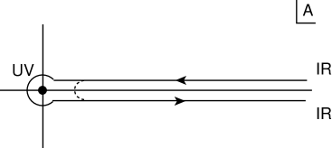
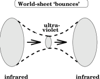
Figure 2: Left Picture: Steepest-descent curve for Liouville zero mode path integration, in the complex plane obtained after complexifying the world-sheet area $A$. Upon the identification of this mode with target time, such curves resemble closed time paths of non equilibrium field theories, in agreement with the non-equilibrium nature of the Liouville string. Right Picture: The “breathing world-sheet”, as a result of the path on the left. The target-space irreversibility arises from a “bounce” interpretation of this process.

Formally, in Liouville strings, the world-sheet correlators of vertex operators are identified with well-defined $-matrix elements rather than scattering amplitudes. The non-factorisability of the $-matrix into proper S-matrix amplitudes, $$\neq SS^{\dagger}$, is obtained by noting that in Liouville strings, which by definition propagate on non-conformal backgrounds, one may define the Liouville zero mode world-sheet path integral in a steepest-descent fashion by means of the curve indicated in figure 2kogan ; emntheory ; mavro . Upon the identification of the Liouville zero mode with time, such a curve resembles closed-time-paths in non-equilibrium field theories. It is the short-distance world-sheet singularities (UV) near the origin of the curve of fig. 2 that cause the aforementioned non factorizability of the $ matrix. One may link the breathing world sheet, arising from the steepest-descent path of the Liouville mode, to a “bounce” on the infrared (IR, large world-sheet area) limitkogan , implying an irreversible RG flow from the ultraviolate to infrared fixed points of the world-sheet system. Details are given in the literatureemntheory ; mavro , where we refer the interested reader for details. For our purposes we only mention that this property links the time irreversibility of the Liouville mode, stemming from world-sheet RG properties, to fundamental properties of space-time $-matrix elements, in a similar fashion to the analysis in wald .

The theory space “coordinates”/backgrounds fields $g^{i}$ become quantum operators upon summing up world-sheet genera emntheory ; decoherence in this theory space is induced precisely by the non vanishing $\beta$-functions, that is the departure from the conformal point emntheory . To see this one invokes the principle of world-sheet renormalization group invariance of target-space quantities with physical significance for the string propagating in such non-conformal backgrounds. One such quantity is the density matrix of this string matter $\rho_{s}$. The RG invariance implies that $\frac{d}{dt}\rho_{s}=0$, where $t\equiv{\rm ln}\mu$ is the world-sheet RG scale.

In the quantum theory this equation reads emntheory ; kogan :

$${\dot{\rho}_{s}}=i[\rho_{s},H]+:\beta^{j}{\cal G}_{ji}[g^{i},\rho_{s}]:$$ (39)

where the overdot denotes partial derivative with respect to $t$, $H$ is the effective low-energy string Hamlitonian, and ${\cal G}_{ij}=z^{2}{\overline{z}}^{2}\langle V_{i}(z)V_{j}(0)\rangle$ is the Zamolodchikov’s metric in “theory space” mavro . The notation $:\dots:$ denotes appropriate ordering of the quantum operators.

Equation (39) has similar form to that of a ‘decoherent evolution’ in the parameter $t$. Clearly, for critical backgrounds $\beta^{i}=0$, and hence the evolution in RG space does not imply any such “decoherence”. However, this decoherence would acquire physical significance only if the identification of the scale $t$ with the real target time variable in string theory holds emntheory . This is not a trivial issue, and in fact it can be shown that it does not hold for any non conformal deformation. However, as already mentioned, there are physically interesting cases, among which strings in de Sitter space times cosmonem , to be discussed separately in the next subsection, or colliding brane cosmologies gravanis , which are non conformal backgrounds in string theory, and in which the above-mentioned identification of time with the world-sheet RG scale, that is the Liouville zero mode, occurs due to dynamical reasons, leading to minimization of energy.

Under such an identification, the RG evolution (39) becomes a real temporal evolution for the reduced density matrix of a string interacting with the non conformal background, which leads to the presence of decoherence terms proportional to the RG $\beta^{i}\neq 0$. Using (39) it can be shownemntheory that such Liouville-string decoherence has the following properties:

(i) Conservation of Probability,

(ii) Von-Neumann entropy monotonic increase: one calculates the relevant rate as:

$$\frac{\partial}{\partial t}\left({\rm Tr}\rho{\rm ln}\rho\right)=\beta^{i}{\cal G}_{ij}\beta^{j}\left({\rm Tr}\rho{\rm ln}\rho\right)$$ (40)

which is positive semi-definite, since $\beta^{i}{\cal G}_{ij}\beta^{j}\geq 0$ due to Zamolodchikov’s c-theorem for unitary theories or its extension for non-unitary oneskutasov .

(iii) Energy conservation on the average, since

$$\frac{\partial}{\partial t}\langle\langle H\rangle\rangle=\frac{\partial}{\partial t}\left(\frac{\partial\beta^{i}}{\partial g^{i}}\right)=0$$ (41)

due to the fact that there is no explicit RG scale $t$ dependence on the $\beta^{i}$ function, due to renormalizability of the $\sigma$-model. However, a word of caution should be placed here. In some cases, in particular logarithmic conformal field theories, such as D-particle recoilkogan , where the short-distance limit of two deformation operators contain explicit logarithms $V_{i}(z)V_{j}(z\textasciiacute)\sim{\rm ln}zc_{ijk}V_{k}/|z-z\textasciiacute|^{2}$, there is explicit $t$ dependence in the Operator Product Expansion coefficients appearing in the perturbative expansion of the $\beta$-function in powers of coupling constants $g^{i}$szabo2 . For instance, in the recoil problem, the anomalous dimension coefficients are $t$-dependentkogan . In such cases, the energy conservation on the average may be spoiled.

This type of Liouville-string decoherence leads to “localisation” in theory space $g^{i}$ emntheory , which can be seen as follows: the RG $\beta$-functions are expressed as a power series in the coordinates/background fields $g^{i}$, $\beta^{i}=C^{i}_{i_{1}\dots i_{n}}g^{i_{1}}\dots g^{i_{n}}$. The linear term is the anomalous dimension term. In a weak field expansion, i.e. when $g^{i}$ are assumed sufficiently weak so that perturbation theory holds, one may assume to a good approximation $\beta^{i}\simeq y_{i}g^{i}$, with $y_{i}$ the anomalous scaling dimension of the $\sigma$-model coupling/background field $g^{i}$. Note also that this is an exact result (in terms of a $g^{i}$ expansion) in some non conformal cosmological backgrounds of string theory, such as de Sitter space, i.e. a space time with a non zero cosmological constant $\Lambda>0$. In such a case, the graviton $\beta$-function, to order $\alpha^{\prime}=M_{s}^{-2}$, with $M_{s}$ the string mass scale, is given by the Ricci tensor: $\beta^{\mu\nu}=\alpha^{\prime}R_{\mu\nu}=\Lambda g_{\mu\nu}$, and thus is linear in the graviton background. We shall examine this case in some detail in the next subsection.

In such linearised cases, one may choose the antisymmetric quantum ordering prescription which leads to a double commutator structure in the theory space coordinate operators $g^{i}$, so that (39) reads:

$${\dot{\rho}_{s}}=i[\rho_{s},H]+\frac{1}{2}y_{i}[g_{i},[g^{i},\rho_{s}]],$$ (42)

where we have used the fact that, to leading order in $g^{i}$, the Zamolodchikov “metric in theory space” ${\cal G}_{ij}\simeq\delta_{ij}+{\cal O}(g^{2})$, which can always be arranged by an appropriate choice of a Renormalization scheme mavro .

Comparing (42) with (14),(17) we observe that we are encountering here exactly an analogous situation, but instead of energy driven or position localisation decoherence models, we have a non-critical string theory induced decoherence. Since $g^{i}$ are generalised “position vectors” in theory space, the same arguments leading to localisation of the state vector in those models will lead here to “localisation in theory space $g^{i}$”. From a physical viewpoint this would imply the emergence of the equilibrium target space of string theories in a dynamical way, due to evolution of a non critical string theory to those equilibrium points. Moreover, the double commutator structure in (42) will also lead to variances $(\Delta g^{i})^{2}$ for the background fields $g^{i}$, expressing the back reaction of string matter on those backgrounds. In the next subsection we shall examine a concrete and physically interesting example of such a situation, that of a de Sitter space time background. As we shall discuss below, in such a case one also obtains an interesting case of CPT Violation of unconventional form, which may be related to some energy-driven decoherence models mentioned abovehoughston ; adler .

2.8 Cosmological CPTV?

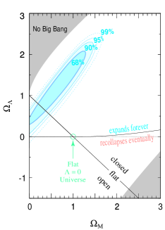
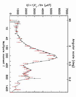
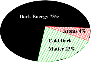
Figure 3: Recent observational evidence for Dark Energy of the Universe (upper left figure: evidence from SnIa (Ref. [54]), upper right figure: evidence from CMB measurements (Ref. [55])) and a pie graph (lower central figure) of the energy budget of our world according to these observations.

One of the reasons that make me prefer the Violation of CPT via the $ matrix decoherence approach over other approaches to CPT Violation, concerns a novel type of CPT Violationat a global scale, which may characterize our Universe. This has been proposed in ref. cosmonem , and was given the name cosmological CPT Violation. This type of CPTV is prompted by recent astrophysical Evidence for the existence of a Dark Energy component of the Universe. For instance, there is direct evidence for a current era acceleration of the Universe, based on measurements of distant supernovae SnIa snIa , which is supported also by complementary observations on Cosmic Microwave Background (CMB) anisotropies (most spectacularly by the recent data of WMAP satellite experiment) wmap .

Best fit models of the Universe from such combined data appear at present consistent with a non-zero, positive cosmological constant $\Lambda\neq 0$. Such a $\Lambda$-universe will eternally accelerate, as it will enter eventually an inflationary (de Sitter) phase again, in which the scale factor will diverge exponentially $a(t)\sim e^{\sqrt{\Lambda/3}t}$, $t\rightarrow\infty$. This implies that there exists a cosmological horizon.

The existence of such horizons implies incompatibility with a S-matrix: no proper definition of asymptotic state vectors is possible, and there is always an environment of d.o.f. crossing the horizon. This situation may be considered as dual to that of a black hole, depicted in fig. 1: in that case the asymptotic observer was in the exterior of the black hole horizon, in the cosmological case the observer is inside the horizon. However, both situations are characterized by the lack of an invertible scattering matrix, hence the above-described theorem by Waldwald on $-matrix and CPTV applies cosmonem , and thus CPT is violated, at a global scale, due to a cosmological constant $\Lambda>0$.

It has been argued in cosmonem that such a violation is described effectively by a modified temporal evolution of matter in such a $\Lambda$-universe, which is given by

$$\partial_{t}\rho=[\rho,H]+{\cal O}(\Lambda M_{s})\rho$$ (43)

where $\Lambda$ is a dimensionless cosmological constant in four dimensions, and $M_{s}$ is the quantum gravity scale (which may be different from the four-dimensional Planck scale, see discussion below).

This form has been derived in the above-described context of non critical strings. Indeed, a de Sitter space time constitutes a non conformal string background, and according to the ideas presented in the previous subsection the temporal evolution of string matter in such a space time is described by the decohering evolution (39). Since, as mentioned previously, the main source of departure from conformal symmetry comes from the graviton $g_{\mu\nu}$ background, whose $\beta^{\mu\nu}=\Lambda g_{\mu\nu}$, one actually has the evolution (42), with the double commutaror structure for the background $g_{\mu\nu}$. The order of the decoherence parameter $\gamma$, then, in such a case is:

$$\gamma\sim\Lambda M_{s}(\Delta g_{\mu\nu})^{2},$$ (44)

where $M_{s}$ is the string scale, and $\Lambda$ is a dimensionless cosmological constant in the $d$-dimensional space time the string propagates on. One may use the modern view point that our four dimensional world is actually a string membrane (D-brane), embedded in a ten-dimensional target (bulk) space. The Standard Model matter is localised on such brane worlds. In the bulk, only fields belonging to the gravitational multiplet of the string spectrum are allowed to propagate. From this view point, then, the string scale $M_{s}$ may be different from the four dimensional Planck scale. However, since string matter is confined on the brane world, it essentially interacts effectively only with the four-dimensional graviton fields, that lie on, or cross, our brane world, and hence one arrives at the estimate (43), with $\Lambda$ the effective four-dimensional cosmological constant on the brane.

An important issue concerns the order of the variance of the metric fluctuations $(\Delta g_{\mu\nu})^{2}$. To arrive at the estimate (43) one has to assume that such variances are of order one. However, there are models of space time foam in string/membrane theoryhorizons ; synchro , where the foam is represented as a gas of D-particle (point-like) defects on three branes, which recoil upon interaction with matter strings. As a result of recoil, there are induced space-time distortions, of the form $g_{0i}\sim u_{i}$, where $i$ is a spatial three-brane index, and $u_{i}$ is the recoil velocity of the D-particle. By momentum conservation, $u_{i}\sim g_{s}\Delta k_{i}/M_{s}$, where $\Delta k_{i}$ is the momentum transfer, which is of order of the incident momentum, $k$, $g_{s}$ is the (weak) string coupling, and $M_{s}/g_{s}$ is the mass of the D-particle. Upon summing world-sheet genera, $u_{i}$ becomes an operator, which acts on energy eigenstates, yielding appropriate eigenvalues of order $g_{s}\Delta k_{i}/M_{s}$.

Considering the case of a two state system, say neutrinos oscillating between two energy states, with the corresponding energy difference arising from a mass-squared difference $\Delta m^{2}$ in the neutrino Hamiltonian $H\simeq p+m^{2}/p+\dots$, one has for the model of horizons :

$$(\Delta g_{0i})^{2}\sim(g_{s}\Delta E/M_{s})^{2}=g_{s}^{2}(\Delta m^{2})^{2}/E^{2}M_{s}^{2}$$ (45)

where $E$ is the energy of the low-energy neutrino interacting with the foam.

From (45) and (39), then, we obtain the order of the decoherence coefficient for this case:

$$\gamma\sim\Lambda g_{s}^{2}(\Delta m^{2})^{2}/E^{2}M_{s}$$ (46)

Comparing with (24) we observe that it is of the same form as in the energy-driven decoherence model of houghston ; adler , provided the decoherence coupling with the environment is of order $\lambda^{2}\sim g_{s}^{2}\Lambda/M_{s}$. In fact, one gets exactly the result (24), if one identifies $M_{s}/g_{s}=M_{P}$, and assumes a $\Lambda\sim 1/g_{s}$, which could be induced by quantum string loop effects (but, of course, this is too big for a realistic cosmological constant). The equivalence with energy driven decoherence of the D-particle foam model should not have come as a surprise, given that the space-time distortion due to the recoil of the D-particle is driven by the energy content of the matter probe, on account of energy conservation.

For realistic values of $\Lambda\sim 10^{-122}$ in Planck units, the above effects are undetectable in any oscillation experiment. Although the order of the cosmological CPTV effects in this scenario is tiny, if we accept that the Planck scale is the ordinary four-dimensional one $M_{P}\sim 10^{-19}$ GeV, and hence undetectable in direct particle physics interactions, however, such cosmological-constant induced CPTV may have already been detected indirectly through the (claimed) observational evidence for a current-era acceleration of the Universe ! Of course, the existence of a cosmological constant brings up other interesting challenges, such as the possibility of a proper quantization of de Sitter space as an open system, which are still unsolved.

At this point I should mention that time Relaxation models for Dark Energy, e.g. quintessence model, where eventually the vacuum energy asymptotes (in cosmological time) an equilibrium zero value, are still currently compatible with the data relax . In such cases it might be possible that there is no cosmological CPTV, since a proper S-matrix can be defined, due to lack of cosmological horizons.

From the point of view of string theory the impossibility of defining a S-matrix in de Sitter space times is very problematic, because critical strings by their very definition depend crucially on such a concept. However, this is not the case of non-critical string theory, which can accommodate in their formalism $\Lambda$ universes cosmonem . It is worthy of mentioning briefly that such non-critical (non-equilibrium) string theory cases are capable of accommodating models with large extra dimensions, in which the string gravitational scale $M_{s}$ is not necessarily the same as the Planck scale $M_{P}$, but it could be much smaller, e.g. in the range of a few TeV. In such cases, the CPTV effects in (43) may be much larger, since they would be suppressed by $M_{s}$ rather than $M_{P}$.

It would be interesting to study further the cosmology of such models and see whether the global type of CPTV proposed in cosmonem , which also entails primordial CP violation of similar order, distinct from the ordinary (observed) CP violation which occurs at a later stage in the evolution of the Early Universe, may provide a realistic explanation of the initial matter-antimatter asymmetry in the Universe, and the fact that antimatter is highly suppressed today. In the standard CPT invariant approach this asymmetry is supposed to be due to ordinary CP Violation. In this respect, I mention that speculations about the possibility that a primordial CPTV space-time foam is responsible for the observed matter-antimatter asymmetry in the Universe have also been put forward in ahluwal but from a different perspective than the one I am suggesting here. In ref. ahluwal it was suggested that a novel CPTV foam-induced phase difference between a space-time spinor and its antiparticle may be responsible for the required asymmetry. Similar properties of spinors may also characterize space times with deformed Poincare symmetries agostini , which may also be viewed as candidate models of quantum gravity. In addition, other attempts to discuss the origin of such an asymmetry in the Universe have been made within the loop gravity approach to quantum gravity singh exploring Lorentz Violating modified dispersion relations for matter probes, especially neutrinos, which we shall discuss below.

3 Phenomenology of CPT Violation

3.1 Order of Magnitude Estimates of CPTV

Before embarking on a detailed phenomenology of CPTV it is worth asking whether such a task is really sensible, in other words how feasible it is to detect such effects in the foreseeable future. To answer this question we should present some estimates of the expected effects in some models of quantum gravity.

The order of magnitude of the CPTV effects is a highly model dependent issue, and it depends crucially on the specific way CPT is violated in a model. As we have seen cosmological (global) CPTV effects are tiny, on the other hand, quantum Gravity (local) space-time effects (e.g. space time foam) may be much larger.

Naively, Quantum Gravity (QG) has a dimensionful constant: $G_{N}\sim 1/M_{P}^{2}$, $M_{P}=10^{19}$ GeV. Hence, CPT violating and decohering effects may be expected to be suppressed by $E^{3}/M_{P}^{2}$ , where $E$ is a typical energy scale of the low-energy probe. This would be practically undetectable in neutral mesons, but some neutrino flavour-oscillation experiments (in models where flavour symmetry is broken by quantum gravity), or some cosmic neutrino future observations might be sensitive to this order: for instance, in models with LV, one expects modified dispersion relations (m.d.r.) which could yield significant effects for ultrahigh energy ($10^{19}$ eV) $\nu$ from Gamma Ray Bursts (GRB) volkov , that could be close to observation. Also in some astrophysical cases, e.g. observations of synchrotron radiation from Crab Nebula or Vela Pulsar, one is able to constraint electron m.d.r. almost near this (quadratic) order synchro .

However, resummation and other effects in some theoretical models may result in much larger CPTV effects of order: $\frac{E^{2}}{M_{P}}$. This happens, e.g., in some loop gravity models loop , or in some (non-critical) stringy models of quantum gravity involving open string excitations emn . Such large effects may already be accessible in current experiments, and most of them are excluded by current observations. Indeed, the Crab nebula synchrotron constraint crab for instance already excludes such effects for electrons. Nevertheless, similar effects for photons are still escaping exclusion at present, and in view of possible violations of the equivalence principle, which might occur in some theoretical models of foamsynchro , according to which only photons are susceptible to such QG-induced m.d.r., the last word on minimal suppression QG effects has not been spoken yet.

On the other hand, as we discussed previously, in some models of decoherence adler one may have single Planck mass suppression, $1/M_{P}$, however the decoherence parameters $\gamma$ depend on the energy variance, rather than the average energy of the probe, $\Delta E=E_{2}-E_{1}$ between, say, the two energy eigenstates of a two-state system, such as neutral kaon, or two-generation neutrino oscillations in hierarchical neutrino models, $\gamma\sim(\Delta E)^{2}/M_{P}$. This will also be undetectable in oscillation experiments in the foreseeable future, despite the minimal Planck scale suppression of the effect in this case.

From the above discussion it is therefore clear that we are in need of guidance by experiment in our quest for the order of decoherence or other non-trivial quantum gravity effects, since theoretically the situation is far from being resolved. Since very little is known about such models, it is important to obtain as much experimental information on bounds of the relevant parameters as possible. Hopefully, this will help us focusing our future research in the phenomenology of quantum gravity on the right track.

3.2 Mnemonic Cubes for CPTV Phenomenology

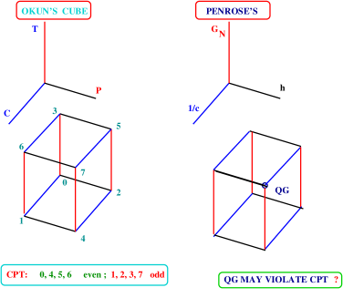
Figure 4: Mnemonic cubes for CPT Violation: Left its phenomenology. Right: its possible theoretical origin.

When CPT is violated there are many possibilities, due to the fact that C,P and T may be violated individually, with their violation independent from one another. This was emphasized by Okun okun some years ago, who presented a set of mnemonic rules for CPTV phenomenology, which are summarized in fig. 4. In this figure I also draw a kind of Penrose cube, indicating where the violations of CPT may come from. The diagram has to be interpreted as follows: CPTV may come from violations of special relativity (axis $1/c$), where the speed of light does not have its value, exhibiting some sort of refractive index in vacuo, or from departure from quantum mechanics (axis $h$), or from gravity considerations, where the gravitational constant departs from its value (axis $G_{N}$), or finally (and most likely) from quantum gravity considerations, where all such effects may coexist.

3.3 Lorentz Violation and CPT: The Standard Model Extension (SME)

We start our discussion on phenomenology of CPT violation by considering CPTV models in which requirement (iii) of the CPT theorem is violated, that is Lorentz invariance. As mentioned previously, such a violation may be a consequence of quantum gravity fluctuations. In this case Lorentz symmetry is violated (LV) and hence CPT, but there is no necessarily quantum decoherence or unitarity loss. Phenomenologically, at low energies, such a LV will manifest itself as an extension of the standard model in (effectively) flat space times, whereby LV terms will be introduced by hand in the relevant lagrangian, with coefficients whose magnitude will be bounded by experiment kostel .

Such SME lagrangians may be viewed as the low energy limit of some string theory vacua, in which some tensorial fields acquire non-trivial vacuum expectation values $<A_{\mu}>\neq 0~{},<T_{\mu_{1}\dots\mu_{n}}>\neq 0.$ This implies a spontaneous breaking of Lorentz symmetry by these (exotic) string vacua kostel .

The simplest phenomenology of CPTV in the context of SME is done by studying the physical consequences of a modified Dirac equation for charged fermion fields in SME. This is relevant for phenomenology using data from the recently produced antihydrogen factories antihydro ; mavroyoko .

In these lectures I will not cover this part in detail, as I will concentrate mainly on neutrinos within the SME context. It suffices to mention that for free hydrogen $H$ (anti-hydrogen ${\overline{H}}$) one may consider the spinor $\psi$ representing electron (positron) with charge $q=-|e|(q=|e|)$ around a proton (antiproton) of charge $-q$, which obeys the modified Dirac equation (MDE):

$$(i\gamma^{\mu}D^{\mu}-M-a_{\mu}\gamma^{\mu}-b_{\mu}\gamma_{5}\gamma^{\mu}-$$

$$-\frac{1}{2}H_{\mu\nu}\sigma^{\mu\nu}+ic_{\mu\nu}\gamma^{\mu}D^{\nu}+id_{\mu\nu}\gamma_{5}\gamma^{\mu}D^{\nu})\psi=0$$ (47)

where $D_{\mu}=\partial_{\mu}-qA_{\mu}$, and $A_{\mu}=(-q/4\pi r,0)$ is the Coulomb potential. CPT & Lorentz violation is described by terms with parameters $a_{\mu}~{},b_{\mu}~{},$ while Lorentz violation only is described by the terms with coefficients $c_{\mu\nu}~{},d_{\mu\nu}~{},H_{\mu\nu}$.

One can perform spectroscopic tests on free and magnetically trapped molecules, looking essentially for transitions that were forbidden if CPTV and SME/MDE were not taking place. The basic conclusion is that for sensitive tests of CPT in antimatter factories frequency resolution in spectroscopic measurements has to be improved down to a range of a 1 mHz, which at present is far from being achieved mavroyoko .

Since the presence of LV interactions in the SME affects dispersion relations of matter probes, other interesting precision tests of such extensions can be made in atomic and nuclear physics experiments, exploiting the fact of the existence of a preferred frame where observations take place. The results and the respective sensitivities of the various parameters appearing in SME are summarized in the table of figure 5, taken from ref. bluhm . As we see, the frame dependence of such LV effects leads to very stringent bounds of the values of the LV parameters in some cases, which are far more superior than the corresponding bounds obtained at present in antihydrogen factories.

Figure 5: Sensitivities of CPTV and LV parameters appearing in SME/Modified Dirac equation for charged probes, from various atomic and nuclear physics experiments.

3.4 Direct SME Tests and Modified Dispersion relations (MDR)

Many LV Models of Quantum Gravity (QG) predict modified dispersion relations relations (MDR) for matter probes, including neutrinos $\nu$ emnnature ; volkov ; grb . This leads to one important class of experimental tests using $\nu$: each mass eigenstate of $\nu$ has QG deformed dispersion relations, which may, or may not, be the same for all flavours:

$$E^{2}={\vec{k}}^{2}+m_{i}^{2}+f_{i}(E,M_{qg},{\vec{k}})~{},\qquad{\rm e.g.}~{}f_{i}=\sum_{\alpha=1,2...}C_{\alpha}{\vec{k}}^{2}\left(\frac{|{\vec{k}}|}{M_{qg}}\right)^{\alpha}$$ (48)

There are stringent bounds on $f_{i}$ from oscillation experiments, as we shall discuss below.

It must be stressed that such MDR also characterize SME, although the origin of MDR in the approach of emnnature ; volkov ; grb is due to an induced non-trivial microscopic curvature of space time as a result of a back reaction of matter interacting with a stringy space time foam vacuum. This is to be contrasted with the SME approach kostel , where the analysis is done exclusively on flat Minkowski space times, at a phenomenological level.

In general there are various experimental tests that can set bounds on MDR parameters, which can be summarized as follows:

(i) astrophysics tests - arrival time fluctuations for photons (model independent analysis of astrophysical GRB data grb

(ii) Nuclear/Atomic Physics precision measurements (clock comparison, spectroscopic tests on free and trapped molecules, quadrupole moments etc) bluhm .

(iii)antihydrogen factories (precision spectroscopic tests on free and trapped molecules: e.g. $1S\rightarrow 2S$ forbidden transitions) mavroyoko ,

(iv) Neutrino mixing and spin-flavour conversion, a brief discussion of which we now turn to.

3.5 Neutrinos and SME

The SME formalism naturally includes the neutrino sector. Recently a SME-LV+CPTV phenomenological model for neutrinos has been given in mewes . The pertinent lagrangian terms are given by:

$${\cal L}^{\nu}_{SME}\ni\frac{1}{2}i{\overline{\psi}}_{a,L}\gamma^{\mu}D_{\mu}\psi_{a,L}-(a_{L})_{\mu ab}{\overline{\psi}}_{a,L}\gamma^{\mu}\psi_{b,L}+$$

$$\frac{1}{2}i(c_{L})_{\mu\nu ab}{\overline{\psi}}_{a,L}\gamma^{\mu}D^{\nu}\psi_{b,L}$$ (49)

where $a,b$ are flavour indices. The model has (for simplicity) no $\nu$-mass differences. Notice that the presence of LV induces directional dependence (sidereal effects)!

To analyze the physical consequences of the model, one passes to an Effective Hamiltonian mewes

$$(H_{\rm eff})_{ab}=|{\vec{p}}|\delta_{ab}+\frac{1}{|{\vec{p}}|}((a_{L})^{\mu}p_{\mu}-(c_{L})^{\mu\nu}p_{\mu}p_{\nu})_{ab}$$ (50)

Notice that $\nu$ oscillations are now controlled by the (dimensionless) quantities $a_{L}L$ & $c_{L}LE$ where L is the oscillation length. This is to be contrasted with the conventional case, where the relevant parameter is associated necessarily with a $\nu$-mass difference $\Delta m$: $\Delta m^{2}L/E$.

There is an important feature of the SME/$\nu$: despite CPTV, the oscillation probabilities are the same between $\nu$ and their antiparticles, if there are no mass differences between $\nu$ and ${\bar{\nu}}$: $P_{\nu_{x}\rightarrow\nu_{y}}=P_{{\bar{\nu}_{x}}\rightarrow{\bar{\nu}_{y}}}$.

Experimentally, it is possible to bound LV+CPTV SME parameters in the neutrino sector with high sensitivity, if we use data from high energy long baseline experiments mewes . Indeed, from the fact that there is no evidence for $\nu_{e,\mu}\rightarrow\nu_{\tau}$ oscillations, for instance, at $E\sim 100$ GeV , $L\sim 10^{-18}$ GeV^-1 we conclude that $a_{L}<10^{-18}$ GeV, $c_{L}<10^{-20}$.

Similarly for an explanation of the LSND anomaly lsnd , claiming evidence for oscillations between (${\bar{\nu}_{\mu}}-{\bar{\nu}_{e}}$) but not for the corresponding neutrinos, a mass-squared difference of order $\Delta m^{2}=10^{-19}$ GeV${}^{2}=10^{-1}$ eV² is required, which implies that $a_{L}\sim 10^{-18}$ GeV, $c_{L}\sim 10^{-17}$. This would affect other experiments, and in fact one can easily come to the conclusion that SME/$\nu$ does not offer a good explanation for LSND, if we accept the result of that experiment as correct, which is not clear at present.

A summary of the Experimental Sensitivities for $\nu$’s SME parameters are given in the table of figure 6, taken from mewes .

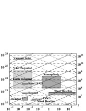
Figure 6: Approximate experimental sensitivities for SME for neutrinos. Lines of constant $L/E$ (solid), $L$ (dashed), and $LE$ (dotted) are shown, which give sensitivities to $\Delta m^{2}$, $a_{L}$, and $c_{L}$, respectively.

3.6 Lorentz non-invariance, MDR and $\nu$-oscillations

Models of quantum gravity predicting MDR of the type (48) for neutrinos volkov ; alfaro , with a leading order $E^{2}/M_{qg}$ modification, can be severely constrained by a study of the induced oscillations between neutrino flavours, as a result of the departure from the standard dispersion relations provided that the quantum-gravity foam responsible for the MDR breaks flavour symmetry, which however is not always the case emnnu .

Figure 7: Shown for each experiment are: (i) operation status, (ii) mean value of observed $\nu$ energy, (iii) the oscillation length $L$, (iv) typical $\nu$-flight distance $X$, and the ratio $\alpha=L/X$, which, in models where the foam induces $\nu$ flavour oscillations, coincides with the phenomenological parameter that controls the size of MDR effects.

This approach has been followed in eichler , where it was shown that if flavour symmetry is not protected in such MDR models, then the extra terms in (48), proportional to $E^{2}/M_{qg}$ will induce an oscillation length $L\sim 2\pi M_{qg}/(\alpha E^{2})$, where $\alpha$ is a phenomenological parameter that controls the size of the effect. This should be contrasted to the Lorentz Invariant case where $L_{\rm LI}\sim 4\pi E/\Delta m^{2}$, with $\Delta m^{2}$ the square mass difference between neutrino flavours. From a field theoretic view point, terms in MDR proportional to some positive integer power of $E^{2}/M_{qg}$ may behave as non-renormalizable operators, for instance, dimension five myers in the case of leading order QG effects suppressed only by a single power of $M_{qg}$.

The sensitivity of the various neutrino oscillation experiments to the parameter $\alpha$ is shown in figure 7 eichler . The conclusion from such analyses, therefore, is that, if the flavour number symmetry is not protected in such MDR foam models with minimal $1/M_{P}$ suppression in the correction terms, then neutrino observatories and long base-line experiments should have already observed such oscillations. As remarked above, however, not all foam models that lead to such MDR predict such oscillations emnnu , and hence such constraints are highly foam-model dependent.

3.7 Lorentz Non Invariance, MDR and $\nu$ spin-flavor conversion

An interesting consequence of MDR in LV quantum gravity theories is associated with modifications to the well-known phenomenon of spin-flavour conversion in $\nu$ interactions lambiase . To be specific, we shall consider an example of a MDR for $\nu$ provided by a Loop Gravity approach to quantum gravity. According to such an approach, the dispersion relations for neutrinos are modified to alfaro :

$$E^{2}_{\pm}=A_{p}^{2}p^{2}+\eta p^{4}\pm 2\lambda p+m^{2}$$ (51)

where $A_{p}=1+\kappa_{1}\frac{\ell_{P}}{{\cal L}},~{}\eta=\kappa_{3}\ell^{2}_{P},~{}\lambda=\kappa_{5}\frac{\ell_{P}}{2{\cal L}^{2}}$, and ${\cal L}$ is a characteristic scale of the problem, which can be either (i) ${\cal L}\sim E^{-1}$, or (ii) ${\cal L}$=constant.

It has been noted in lambiase that such a modification in the dispersion relation will affect the form of the spin-flavour conversion mechanism. Indeed, it is well known through the Mikheyev-Smirnov-Wolfenstein (MSW) effect msw that Weak interaction Effects of $\nu$ propagating in a medium result in an energy shift $\sqrt{2}G_{F}(2n_{e}-n_{n})$, where $n_{e}(n_{n})$’s denote electron (neutron) densities. In addition to such effects, one should also take into account the interaction of $\nu$ with external magnetic fields, $B$, via a radiatively induced magnetic moment $\mu$, corresponding to a term in the effective lagrangian: ${\cal L}_{\rm int}=\mu{\overline{\psi}}\sigma^{\mu\nu}F_{\mu\nu}\psi$, with $\psi$ the neutrino fermionic field.

According to the standard theory, the equation for evolution describing the spin-flavour conversion phenomenon due to the above-described medium and magnetic moment effects for, say, two neutrino flavours ($\nu_{e},\nu_{\mu}$) is given by:

$$i\frac{d}{dr}\left(\begin{array}[]{c}\nu_{eL}\\ \nu_{\mu L}\\ \nu_{eR}\\ \nu_{\mu R}\end{array}\right)={\cal H}\left(\begin{array}[]{c}\nu_{eL}\\ \nu_{\mu L}\\ \nu_{eR}\\ \nu_{\mu R}\end{array}\right)~{},$$ (60)

where the effective Hamiltonian ${\cal H}$ should be corrected in the loop gravity case to take into account $\lambda$-effects, associated with MDR (51):

$${\cal H}=\left(\begin{array}[]{cccc}-\frac{\Delta m^{2}}{4p}{\rm cos}2\theta-\lambda+\sqrt{2}G_{F}n_{e}&\frac{\Delta m^{2}}{4p}{\rm sin}2\theta&\mu_{ee}B&\mu B\\ \frac{\Delta m^{2}}{4p}{\rm sin}2\theta&\frac{\Delta m^{2}}{4p}{\rm cos}2\theta-\lambda+\sqrt{2}G_{F}n_{e}&\mu B&\mu_{\mu\mu}B\\ \mu_{ee}B&\mu B&-\frac{\Delta m^{2}}{4p}{\rm cos}2\theta+\lambda&\frac{\Delta m^{2}}{4p}{\rm sin}2\theta\\ \mu B&\mu_{\mu\mu}B&\frac{\Delta m^{2}}{4p}{\rm sin}2\theta&\frac{\Delta m^{2}}{4p}{\rm cos}2\theta+\lambda\end{array}\right)$$ (61)

where $\mu\equiv\mu_{e\mu}$, $\Delta m^{2}=m_{2}^{2}-m_{1}^{2}$, and $B$ is the magnetic field. We should notice at this stage that the above formalism refers to Dirac $\nu$; for Majorana $\nu$ one should replace: $\nu_{iL}\rightarrow\nu_{i}$, $\nu_{iR}\rightarrow{\overline{\nu}}_{i}$. Details can be found in lambiase .

For our purposes we note that the Resonant Conditions for Flavour-Spin-flip are lambiase :

$$\nu_{eL}\rightarrow\nu_{\mu R}:\quad 2\lambda+\frac{\Delta m^{2}}{2p}{\rm cos}2\theta-\sqrt{2}G_{F}n_{e}(r_{res})=0$$

$$\nu_{\mu L}\rightarrow\nu_{eR}:\quad 2\lambda-\frac{\Delta m^{2}}{2p}{\rm cos}2\theta-\sqrt{2}G_{F}n_{e}(r_{res})=0~{}.$$ (62)

One can use the above conditions to obtain bounds for $\lambda,\kappa_{i}$ via the oscillation probabilities for spin-flavour conversion:

$$P_{\nu_{eL}\rightarrow\nu_{\mu R}}=\frac{1}{2}(1-{\rm cos}2{\tilde{\theta}}{\rm cos}2\theta)~{},$$ (63)

where ${\rm tan}2{\tilde{\theta}}(r)=\frac{4\mu B(r)E}{|\Delta m^{2}|{\rm cos}2\theta-4E\lambda+2\sqrt{2}G_{F}En_{e}(r)}$.

To obtain these bounds the author of lambiase made the following physically relevant assumptions: (a) Reasonable profiles for solar $n_{e}\sim n_{0}e^{-10.5r/R_{\odot}}$, $n_{0}=85N_{A}{\rm cm}^{-3}$. (b) Also: $\mu\sim 10^{-11}\mu_{B}$. Then, an upper bound on $\lambda$ is obtained of order: $\lambda\leq\frac{1}{2}\left(10^{-12}e^{-10.5r_{res}/R_{\odot}}{\rm eV}+\frac{|\Delta m^{2}|}{2E}\right)$.

To obtain bounds on $\kappa$ we need to distinguish two cases:

(I) ${\cal L}$=universal constant: In this case, we already know from photon dispersion tests on GRB and (AGN) grb ; alfaro that ${\cal L}\sim 10^{-18}$ eV^-1. Then, from best-fit solar $\nu$-oscillations induced by MSW, one may use experimental values of $\Delta m^{2}$, ${\rm sin}^{2}2\theta$, and obtain the following bound on $\kappa_{i}$: $\kappa_{5}<10^{-25}$. From atmospheric oscillations, in particular LSND experiment lsnd , $\nu_{\mu}\rightarrow\nu_{e}$ fits the data with: $|\Delta m^{2}|\sim eV^{2}$, ${\rm sin}^{2}2\theta\sim(0.2-3)\times 10^{-3}$, $E_{\rm max}\sim 10$ MeV, then $\kappa_{5}<10^{-17}$.

(II) ${\cal L}\sim p^{-1}$ a mobile scale: In that case, from SOLAR oscillations, with $p\sim 1-10{\rm MeV}$ one gets $\kappa_{5}={\cal O}(1-100)$, which is a natural range of values from a quantum-gravity view point. From atmospheric oscillations, for the maximum $\nu$ $E\sim 10$ MeV, and ${\cal L}\sim E^{-1}$, one obtains $\kappa_{5}\sim 10^{4}$, which is a very weak bound.

The conclusion from these considerations, therefore, is that the experimental data seem to favour case (II), at least from a naturalness point of view.

3.8 $\nu$-flavour states and modified Lorentz Invariance (MLI)

An interesting recent idea blama , which we would like to discuss now briefly, arises from the observation of the peculiar way in which flavour $\nu$ states experience Lorentz Invariance. Indeed, neutrino flavour states are a superposition of mass eigenstates with standard dispersion relations of different mass. If one computes the expectation value of the Hamiltonian with respect to flavour states, e.g. in a simplified two-flavour scenario discussed in blama , then one finds:

$$E_{e} = <\nu_{e}|H|\nu_{e}>=\omega_{k,1}{\rm cos}^{2}\theta+\omega_{k,2}{\rm sin}^{2}\theta~{},$$

$$E_{\mu} = <\nu_{\mu}|H|\nu_{\mu}>=\omega_{k,2}{\rm cos}^{2}\theta+\omega_{k,1}{\rm sin}^{2}\theta~{},$$ (64)

with $\theta$ the mixing angle.

One has: $H|\nu_{i}>=\omega_{i}|\nu_{i}>$, $i=1,2$, where the $\omega_{k,i}=\sqrt{{\vec{k}}^{2}+m_{i}^{2}}$ is a standard dispersion relation. However, since the sum of two square roots in not in general a square root, one concludes that flavour states do not satisfy the standard dispersion relations. In general this poses a problem, as it would naively imply the introduction of a preferred frame, due to an apparent violation of the standard linear Lorentz symmetry.

The idea of blama , whose validity of course remains to be seen, but which I find rather intriguing, and this is why I decided to include it in these lectures, is to avoid using preferred frames by introducing instead non-linearly modified Lorentz transformations to account for the modified dispersion relations of the flavour states. The idea is formally similar, but physically very different, to the approach of nlls , in which, in order to ensure observer independence of the Planck length, viewed as an ordinary length in quantum gravity, and not as a universal coupling constant, one has to modify non linearly the Lorentz transformations. The result is that flavour states satisfy the following MDR:

$$E_{i}^{2}f_{i}^{2}(E_{i})-{\vec{k}}^{2}g_{i}^{2}(E_{i})=M_{i}^{2}\quad i=e,\mu$$ (65)

One can determine blama the $f_{i}(E_{i},\theta,m_{i}),g_{i}(E_{i},\theta,m_{i}),M_{i}(m_{i},\theta)$ by comparing with $E_{i}=E_{(}\omega_{i},m_{i})$ above ((c.f. (64)).

Then, in the spirit of nlls , one can identify the non-linear Lorentz transformation that leaves the MDR (65) invariant: $U\circ(E,{\vec{k}})=(Ef,{\vec{k}}g)$.

Figure 8: Left: Tail of tritium $\beta$-decay spectrum, for massless $\nu$ (solid) and for LI flavour states (dashed and dot-long-dashed). Also plotted is the preferred frame case. Right: Likelihood Contours of $M^{2}$ (in units of $m_{2}^{2}$) upon which $\beta$-decay depends.

The interesting feature is that these ideas can be tested experimentally, e.g. in $\beta$-decay experiments: $N_{1}\rightarrow N_{2}+e^{-}+{\bar{\nu}}_{e}$, where e.g. $N_{1}=~{}^{3}{\rm H}$, $N_{2}=~{}^{3}{\rm He}$.

Energy conservation in conventional $\beta$-decay implies: $E_{N_{1}}=E_{N_{2}}+E+E_{e}$, where $E$ is the energy of $e$, which would unavoidably introduce a preferred frame. However, in the non-linear LI case for flavour states, where the use of preferred frame is avoided, this relation is modified blama : $E_{N_{1}}=E_{N_{2}}+E+E_{e}f_{e}(E_{e})$.

These two choices are reflected in different predictions for the endpoint of the $\beta$-decay, that is the maximal kinetic energy the electron can carry (c.f. figure 8). We refer the interested reader to blama for further discussion on the experimental set up to test these ideas.

From the point of view of CPTV, which is our main topic of discussion here, I must mention that in such non-linearly modified Lorentz symmetry cases it is not clear what form the CPT theorem, if any, takes. This is currently under investigation waldron . In this sense, the link between CPTV and modified flavour-state dispersion relations, and therefore the interpretation of the associated experiments from this viewpoint, are issues which are not yet clear.

3.9 CPTV and Departure from Locality for Neutrinos

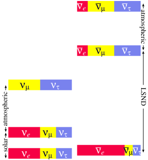
Figure 9: The CPTV neutrino spectrum proposed by Murayama-Yanagida to explain LSND. One needs $m^{2}_{\nu}-m^{2}_{\bar{\nu}}\sim 0.1~{}{\rm ev}^{-2}=10^{-19}~{}{\rm GeV}^{2}$.

As another way of violating CPT one can relax the requirement of locality. This idea has been pursued in barenboim , in an attempt to present a concrete model for CPT Violation for neutrinos, with CPTV Dirac masses, in an attempt to explain the LSND anomalous results lsnd , according to which there is experimental evidence for oscillations in the antineutrino sector, ${\overline{\nu}}_{e}\rightarrow{\overline{\nu}}_{\mu}$, but not in the corresponding neutrino one. In fact, the idea of invoking CPTV Dirac mass spectra for neutrinos in order to account for the LSND results without invoking a sterile neutrino is due to the authors of mura (see figure 9). However no concrete theoretical model was presented there.

The model lagrangian of barenboim reads:

$$S=\int d^{4}x{\bar{\psi}}i\partial_{\mu}\gamma^{\mu}\psi+\frac{im}{2\pi}\int d^{3}xdtdt^{\prime}{\bar{\psi}}(t)\frac{1}{t-t^{\prime}}\psi(t^{\prime})$$ (66)

The on shell equations (in momentum space) for the (Dirac) spinors are:

$$(p_{\mu}\gamma^{\mu}-m\epsilon(p_{0}))u_{\pm}(p)=0~{},$$ (67)

with $\epsilon(p_{0})$ the sign function, and

$$\psi_{+}(x)=u_{+}(p)e^{-ip\cdot x},\qquad p^{2}=m^{2},~{}p_{0}>0$$

$$\psi_{-}(x)=u_{-}(p)e^{-ip\cdot x},\qquad p^{2}=m^{2},~{}p_{0}<0$$ (68)

Notice that on-shell Lorentz invariance is maintained due to the presence of $(\epsilon(p_{0})$) but is relaxed.

As remarked in greenb , however, the model of barenboim , although respecting Lorentz symmetry on-shell, has correlation functions (which are in general off-shell quantities) that do violate Lorentz symmetry, in the sense that they transform non covariantly under Lorentz transformations. Therefore, the CPTV in this model is ultimately connected to LV.

The two-generation non-local model of barenboim seems to be marginally disfavoured by the current neutrino data, as claimed in strumia (see figure 10).

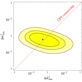
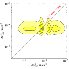
Figure 10: Left: Atmospheric $m_{\nu}-m_{\overline{\nu}}$ (68, 90, 99 %, 2 d.o.f.). Right: For solar & reactor data (68, 90, 99 %, 2 d.o.f.).

$$\begin{array}[]{lc|cccc}\lx@intercol\hfil\hbox{model \& no.\ of free parameters}\hfil\lx@intercol\vrule\lx@intercol&\Delta\chi^{2}&\hbox{mainly incompatible with}&\hbox{main future test}\\ \hline\cr\lx@intercol\hfil\hbox{ideal fit (no known model)}\hfil\lx@intercol\vrule\lx@intercol&0&&?\\ \Delta L=2\hbox{ decay }\bar{\mu}\rightarrow\bar{e}\bar{\nu}_{\mu}\bar{\nu}_{e}&6&12&\hbox{\sc Karmen}&\hbox{TWIST}\\ 3+1:~{}\Delta m^{2}_{\rm sterile}=\Delta m^{2}_{\rm LSND}&9&6+9?&\hbox{{\sc Bugey} + cosmology?}&\hbox{\sc MiniBoone}\\ \hbox{3 $\nu$ and CPTV~{} (no $\Delta\bar{m}^{2}_{\rm sun}$)}&10&15&\hbox{KamLAND}&\hbox{\sc KamLAND}\\ \hbox{3 $\nu$ and CPTV~{} (no $\Delta\bar{m}^{2}_{\rm atm}$)}&10&25&\hbox{SK atmospheric}&\hbox{$\bar{\nu}_{\mu}$ LBL?}\\ \hbox{normal 3 neutrinos}&5&25&\hbox{LSND}&\hbox{\sc MiniBoone}\\ 2+2:~{}\Delta m^{2}_{\rm sterile}=\Delta m^{2}_{\rm sun}&9&30&\hbox{SNO}&\hbox{SNO}\\ 2+2:~{}\Delta m^{2}_{\rm sterile}=\Delta m^{2}_{\rm atm}&9&50&\hbox{SK atmospheric}&\hbox{$\nu_{\mu}$ LBL}\\ \end{array}$$

Table 1: Interpretations of solar, atmospheric and LSND data, ordered according to the quality of their global fit. A $\Delta\chi^{2}=n^{2}$ roughly signals an incompatibility at $n$ standard deviations.

A summary of data and interpretations of current models, including those which entail CPT violation is given in Table 1, taken from the first paper in strumia . In that paper it has also been claimed that the recent WMAP wmap data on neutrinos seem to disfavour 3 + 1 scenaria which conserve CPT invariance. In my opinion one has to wait for future data from WMAP, before definite conclusions on this issue are reached, given that the current WMAP data are rather crude in this respect. I will not go further into a detailed discussion of this topic, as such summaries of neutrino data and their interpretations can be found in the literature, where I refer the interested reader smirnov .

Before closing this section, I would like to remark that most of the theoretical analyses for QG-induced CPTV in neutrinos have been done in simplified two-flavour oscillation models. Including all three generations in the formalism may lead to differences in the corresponding conclusions regarding sensitivity (or conclusions about exclusion) of the associated CPTV effects. In this respect the measurements of the mixing angle angle $\theta_{13}$ in the immediate future minos , as a way of detecting generic three-flavour effects, will be very interesting. In the current phenomenology, CPT invariance is assumed for the theoretical estimates of this parameter lindner .

3.10 Four-generation $\nu$ models with CPTV

Figure 11: Upper bound (solid) on the $\nu_{\mu}\rightarrow\nu_{e}$ oscillation amplitude $4|U_{e4}|^{2}|U_{\mu 4}|^{2}$ from the GALLEX limit on $|U_{e4}|$ and the CDHSW limit on $|U_{\mu 4}|$ (90% C. L. results are used in both cases). The dot-dashed line is the 99% C. L. upper bound from Bugey and CDHSW if $CPT$ is conserved. Also shown are the expected sensitivity (dashed) of the MiniBooNE experiment and, for comparison, the allowed region (within the dotted lines) for $4|\bar{U}_{e4}|^{2}|\bar{U}_{\mu 4}|^{2}$ from a combined analysis of LSND and KARMEN data, both at the 90% C. L.

A natural question arises at this point, concerning ($3+1$ or $2+2$) $\nu$ scenaria which violate CPT symmetry. This issue has been studied recently in barger . These authors postulated a model for CPTV with four generations for neutrinos which leads to different flavor mixing between $\nu$, ${\bar{\nu}}$: $\nu_{a}=\sum_{i=1}^{4}U^{*}_{ai}\nu_{i},\qquad{\bar{\nu}}_{a}=\sum_{i=1}^{4}{\bar{U}}_{ai}{\bar{\nu}}_{i},$ with $U\neq{\bar{U}}$ due to CPTV. There are various cases to be studied:

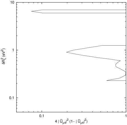
Figure 12: Lower bounds on $4|\bar{U}_{\mu 4}|^{2}(1-|\bar{U}_{\mu 4}|^{2})$ (the amplitude for atmospheric $\bar{\nu}_{\mu}$ survival at the LSND mass scale) from the Bugey limit on $\bar{\nu}_{e}$ disappearance and the $\bar{\nu}_{\mu}\rightarrow\bar{\nu}_{e}$ oscillation amplitude indicated by LSND and KARMEN (90% C. L. results are used in both cases).

• 3 + 1 models (see figs. 11,12): one $\nu$ mass well separated from others, sterile $\nu$ couples only to isolated state. The relevant Oscillation probabilities are: $P_{\nu_{i}\rightarrow\nu_{i}}(|U_{ij}|^{2})\neq P_{{\bar{\nu}}_{i}\rightarrow{\bar{\nu}}_{i}}(|{\bar{U}}_{ij}|^{2})$

  Experimentally one may bound $|{\bar{U}}_{e4}|$ and $U_{\mu 4}$ but there are no tight constraints for $|{\bar{U}}_{\mu 4}|$, $U_{e4}$. This is to be contrasted with (3 + 1)$\nu$ CPT conserving models where $U={\bar{U}}$. Hence (3 + 1)$\nu$ + CPTV seems still viable.

• 2 + 2 models (see fig. 13): sterile $\nu$ couples to solar and atmospheric $\nu$ oscillations. This structure is only permitted in ${\bar{\nu}}$ sector. Even with CPT Violation, however, 2+2 models are strongly disfavoured by data.

Figure 13: Constraints on sterile neutrino mixing angles $\alpha$ and $\bar{\alpha}$ from (solid line) and (dashed line) data. The dotted line is the prediction if $CPT$ is conserved.

Although the introduction of a fourth neutrino generation with CPTV within conventional field theory seems to be consistent with the current neutrino data, however, there seems to be no concrete evidence for a forth generation from any experiment to date, including the most recent astrophysical WMAP data, as we have seen above. This prompts one to examine alternative ways of explaining the current neutrino “anomalous data”, like LSND, employing unconventional ways of CPT Violation by means of quantum decoherence, which are in principle independent of mass differences between particle and antiparticles.

In the next subsection we shall be dealing with this topic, reviewing first the relevant phenomenological formalism which allows direct comparison with experiment. I will start with the phenomenology of CPT violation in neutral mesons and neutrons, as a historical introduction to the general reader, and then I will proceed to the neutrino case. I shall argue that minimal decoherence models with CPTV differences in the decoherence parameters between particle and antiparticle sectors, but not CPTV mass differences, can account for all existing neutrino data, including LSND results, without the need for enlarging the neutrino sector, that is staying within three generation models.

3.11 CPTV through QG Decoherence: Neutral Mesons

In this subsection I will discuss CPTV through decoherence, which is my preferred way of QG-induced CPTV. As mentioned above, in this case the matter systems are viewed as open quantum mechanical or quantum-field theoretic systems interacting with a gravitational ‘environment’, consisting of degrees of freedom inaccessible to low-energy scattering experiments. The presence of such an environment leads to modified quantum evolution, which however is not necessarily Lorentz Violating mill . Thus, such an approach to CPTV should in principle be studied separately, and indeed it is possible for the CPTV decoherence effects to be disentangled experimentally from the LV ones, due to the frame dependence of the latter.

Currently, the most sensitive particle physics probes of such a modification from quantum mechanical behavior (often called ‘quantum mechanics violation’ QMV ehns ; emn ) are: (i) neutral kaons and B-mesons ehns ; emn and $\phi$-, B-factories huet ; benatti1 ; bernabeu (ii) neutron interferometryehns , (iii) ultracold (slow) neutrons in Earth’s gravitational field, and (iv) Neutrino flavour mixing, which is induced independently of masses and mass differences between neutrino species, as we shall discuss below. In these lectures I will discuss briefly (i),(iii) and (iv).

Let us start with the neutral Kaon case. This is a typical two-state system of decoherence. One could follow the Lindblad parametrization benatti1 , in which the requirement of complete positivity would imply a single decoherence parameter $\gamma$. The requirement of energy conservation on the average in such models would then imply the double commutator structure (17) for the decoherence term, which however would depend on the square of the energy variance between the two energy-eigenstates of the neutral Kaon system, as in (24). This would be too small to be detected experimentally in neutral meson experiments and factories in the foreseeable future.

However, as argued in emnlarge , complete positivity may not be valid in generic models of quantum gravity, such as the non-critical string decoherence models (39). Indeed, in that case, the decoherence terms contain the Zamolodchikov metric $\langle V_{i}V_{j}\rangle$ and as such are non-linear in the probe state density matrix $\rho$, given that $\langle\dots\rangle={\rm Tr}(\rho\dots)$ depends on it. Complete positivity for non-linear effective theories (e.g. Hartree-Fock type, mean field approaches) is in general a non well defined concept kunna .

In fact, in the original parametrizationehns of the QG-induced decoherence effects for the neutral Kaon system this requirement has not been imposed. In such a paremetrization, which has also been followed in more recent, and more complete, phenomenological analyses of this system emn ; huet , in addition to the basic principle of entropy increase, one also imposes the requirement of conservation of strangeness by the quantum gravity interactions. This follows from the so-called $\Delta S=\Delta Q$ rule which seems to characterise the leading-order Kaon weak-interaction physics, which in general violates strangeness, but the charge transfer in the neutral Kaon physics is a much more subleading effect than the dominant CP violation effects. This feature is assumed to be obeyed by the quantum gravity interactions ehns , which are thus assume to conserve strangeness to leading order.

According to our general discussion in section 2 on the dynamical-semigroup approach to decoherence, on which the formalism of ref. ehns is based, for the neutral-Kaon two-level system the non-Hamiltonian decoherence term in the evolution equation for $\rho$ can be parametrized by a $4\times 4$ matrix $\delta H\hskip-8.5pt/\hskip 2.0pt_{\alpha\beta}$, where the indices $\alpha,\beta,\dots$ enumerate the Hermitian $\sigma$-matrices $\sigma_{0,1,2,3}$, which we represent in the so-called $K_{1,2}$ basis, defined as $|K^{1,2}\rangle=\frac{1}{\sqrt{2}}\left(|K^{0}\rangle\pm|\overline{K}^{0}\rangle\right)$. In Neutral Kaons, the CP eigenstates are not energy (physical) eigenstates, thereby leading to mixing. We refer the reader to the literature ehns ; emn for details of this description, noting here the following forms for the neutral kaon Hamiltonian

$$H=\left(\begin{array}[]{cc}M-{\textstyle{i\over 2}}\Gamma-{\rm Re}M_{12}+{\textstyle{i\over 2}}{\rm Re}\Gamma_{12}&{\textstyle{1\over 2}}\delta M-{\textstyle{i\over 4}}\delta\Gamma-i{\rm Im}M_{12}-{\textstyle{1\over 2}}{\rm Im}\Gamma_{12}\\ {\textstyle{1\over 2}}\delta M-{\textstyle{i\over 4}}\delta\Gamma+i{\rm Im}M_{12}-{\textstyle{1\over 2}}{\rm Im}\Gamma_{12}&M-{\textstyle{i\over 2}}\Gamma+{\rm Re}M_{12}-{\textstyle{i\over 2}}{\rm Re}\Gamma_{12}\end{array}\right)$$ (69)

in the $K_{1,2}$ basis, or

$$H_{\alpha\beta}=\left(\begin{array}[]{cccc}-\Gamma&-{\textstyle{1\over 2}}\delta\Gamma&-{\rm Im}\Gamma_{12}&-{\rm Re}\Gamma_{12}\\ -{\textstyle{1\over 2}}\delta\Gamma&-\Gamma&-2{\rm Re}M_{12}&-2{\rm Im}M_{12}\\ -{\rm Im}\Gamma_{12}&2{\rm Re}M_{12}&-\Gamma&-\delta M\\ -{\rm Re}\Gamma_{12}&-2{\rm Im}M_{12}&\delta M&-\Gamma\end{array}\right)$$ (70)

in the $\sigma$-matrix basis. Above, $M$ denotes mass parameters, $\Gamma$ denotes widths, and $\delta(\dots)$ denotes CPTV differences between particle and antiparticle sectors, which are due to quantum mechanical effects, such as LV etc..

As mentioned previously, we assume that the dominant violations of quantum mechanics conserve strangeness, so that $\delta H\hskip-8.5pt/\hskip 2.0pt_{1\beta}$ = 0, and that $\delta H\hskip-8.5pt/\hskip 2.0pt_{0\beta}$ = 0 so as to conserve probability. Since $\delta H\hskip-8.5pt/\hskip 2.0pt_{\alpha\beta}$ is a symmetric matrix, it follows that also $\delta H\hskip-8.5pt/\hskip 2.0pt_{\alpha 0}=\delta H\hskip-8.5pt/\hskip 2.0pt_{\alpha 1}=0$. Thus, we arrive at the general parametrization

$${\delta H\hskip-8.5pt/\hskip 2.0pt}_{\alpha\beta}=\left(\begin{array}[]{cccc}0&0&0&0\\ 0&0&0&0\\ 0&0&-2\alpha&-2\beta\\ 0&0&-2\beta&-2\gamma\end{array}\right)$$ (71)

where, as a result of the positivity of the hermitian density matrix $\rho$ ehns

$$\alpha,\gamma>0,\qquad\alpha\gamma>\beta^{2}\ .$$ (72)

We recall emn that the decoherence terms violate CP, given that the latter transformation can be expressed as a linear combination of $\sigma_{2,3}$ in the $K_{1,2}$ basis : ${\rm CP}=\sigma_{3}\cos\theta+\sigma_{2}\sin\theta$, for some choice of phase $\theta$. It is apparent that none of the non-zero terms $\propto\alpha,\beta,\gamma$ in $\delta H\hskip-8.5pt/\hskip 2.0pt_{\alpha\beta}$ (71) commutes with this CP transformation. In other words, each of the three parameters $\alpha$, $\beta$, $\gamma$ violates CP. Moreover, in the problem there is evolution of pure to mixed states, as we shall discuss below, leading, according to the theorem of wald , described above, also to a strong form of CPT Violation. Thus, the decoherent CPTV evolution in the neutral Kaon system leads to a much richer phenomenology than in conventional CPT Violations within a quantum mechanical framework, in the absence of decoherence, where the CPT may be violated only through differences in masses $\delta M$ and widths $\delta\Gamma$ between particles and antiparticles. This is because the symmetric $\delta H\hskip-8.5pt/\hskip 2.0pt$ matrix has three parameters in its bottom right-hand $2\times 2$ submatrix, whereas the $h$ matrix appearing in the time evolution within quantum mechanics has only one complex CPT-violating parameter $\delta$,

$$\delta=-{\textstyle{1\over 2}}\frac{{\textstyle{1\over 2}}\delta\Gamma+i\delta M}{{\textstyle{1\over 2}}|\Delta\Gamma|+i\Delta m}\ ,$$ (73)

where $\delta M$ and $\delta\Gamma$ violate CPT, but do not induce any mixing in the time evolution of pure state vectorsemn . The parameters $\Delta m=M_{L}-M_{S}$ and $|\Delta\Gamma|=\Gamma_{S}-\Gamma_{L}$ are the usual differences between mass and decay widths, respectively, of the long-lived $K_{L}$ and short-lived $K_{S}$ energy (physical) eigenstates. For more details we refer the reader to the literature emn . The above results imply that the experimental constraints pdg on CPT Violation have to be rethought. As we shall discuss later on, there are essential differences between quantum-mechanical CPT Violation and the non-quantum-mechanical CPT violation induced by the effective parameters $\alpha,\beta,\gamma$ ehns .

Useful observables are associated with the decays of neutral kaons to $2\pi$ or $3\pi$ final states, or semileptonic decays to $\pi l\nu$. In the density matrix formalism introduced above, their values are given by expressions of the form ehns ; emn

$$\left\langle O_{i}\right\rangle={\rm Tr}\,[O_{i}\rho]\ ,$$ (74)

where the observables $O_{i}$ are represented by $2\times 2$ hermitian matrices. For instructive purposes we give their expressions in the $K_{1,2}$ basis

$$O_{2\pi} = \left(\begin{array}[]{cc}0&0\\ 0&1\end{array}\right)\ ,\qquad O_{3\pi}\propto\left(\begin{array}[]{cc}1&0\\ 0&0\end{array}\right)\ ,$$ (79)

$$O_{\pi^{-}l^{+}\nu} = \left(\begin{array}[]{cc}1&1\\ 1&1\end{array}\right)\ ,\qquad O_{\pi^{+}l^{-}\bar{\nu}}=\left(\begin{array}[]{rr}1&-1\\ -1&1\end{array}\right)\ .$$ (84)

which constitute a complete hermitian set. As we discuss in detail in emn , it is possible to measure the interferecne between $K_{1,2}$ decays into $\pi^{+}\pi^{-}\pi^{0}$ final states with different CP properties, by restricting one’s attention to part of the phase space $\Omega$, e.g., final states with $m(\pi^{+}\pi^{0})>m(\pi^{-}\pi^{0})$. In order to separate this interference from that due to $K_{S,L}$ decays into final states with identical CP properties, due to CP Violation in the $K_{1,2}$ mass matrix or in decay amplitudes, we consider the difference between final states with $m(\pi^{+}\pi^{0})>m(\pi^{-}\pi^{0})$ and $m(\pi^{+}\pi^{0})<m(\pi^{-}\pi^{0})$. This observable is represented by the matrix

$$O_{3\pi}^{\rm int}=\left(\begin{array}[]{cc}0&{\cal K}\\ {\cal K}^{*}&0\end{array}\right)$$ (85)

where

$${\cal K}\equiv\frac{\left[\int_{m(\pi^{+}\pi^{0})>m(\pi^{-}\pi^{0})}d\Omega-\int_{m(\pi^{+}\pi^{0})<m(\pi^{-}\pi^{0})}d\Omega\right]A_{2}(I_{3\pi}=2)A_{1}(I_{3\pi}=1)}{\int d\Omega|A_{1}(I_{3\pi}=1)|^{2}}$$ (86)

where ${\cal K}$ is expected to be essentially real, so that the $O_{3\pi}^{\rm int}$ observable provides essentially the same information as $O_{\pi^{-}l^{+}\nu}-O_{\pi^{+}l^{-}{\overline{\nu}}}$.

In this formalism, pure $K^{0}$ or ${\bar{K}}^{0}$ states, such as the ones used as initial conditions in the CPLEAR experiment cplear , are described by the following density matrices

$$\rho_{K^{0}}={\textstyle{1\over 2}}\left(\begin{array}[]{cc}1&1\\ 1&1\end{array}\right)\ ,\qquad\rho_{{\bar{K}}^{0}}={\textstyle{1\over 2}}\left(\begin{array}[]{rr}1&-1\\ -1&1\end{array}\right)\ .$$ (87)

We note the similarity of the above density matrices (87) to the semileptonic decay observables in (84), which is due to the strange quark ($s$) content of the kaon $K^{0}\ni{\bar{s}}\rightarrow{\bar{u}}l^{+}{\nu},{\bar{K}}^{0}\ni s\rightarrow ul^{-}\bar{\nu}$, and our assumption of the validity of the $\Delta S=\Delta Q$ rule.

One can apply the above formalism to compute the time evolution of certain quantities that are of relevance to experimentcplear , being directly observable. These are asymmetries associated with decays of an initial $K^{0}$ beam as compared to corresponding decays of an initial ${\bar{K}}^{0}$ beam

$$A(t)=\frac{R({\bar{K}}^{0}_{t=0}\rightarrow{\bar{f}})-R(K^{0}_{t=0}\rightarrow f)}{R({\bar{K}}^{0}_{t=0}\rightarrow{\bar{f}})+R(K^{0}_{t=0}\rightarrow f)}\ ,$$ (88)

where $R(K^{0}\rightarrow f)\equiv{\rm Tr}\,[O_{f}\rho(t)]$, denotes the decay rate into the final state $f$, given that one starts from a pure $K^{0}$ at $t=0$, whose density matrix is given in (87), and $R({\bar{K}}^{0}\rightarrow{\bar{f}})\equiv{\rm Tr}\,[O_{\bar{f}}{\bar{\rho}}(t)]$ denotes the decay rate into the conjugate state ${\bar{f}}$, given that one starts from a pure ${\bar{K}}^{0}$ at $t=0$. One considers the following set of asymmetries: (i) identical final states: $f={\bar{f}}=2\pi$: $A_{2\pi}~{},~{}A_{3\pi}$, (ii) semileptonic : $A_{T}$ (final states $f=\pi^{+}l^{-}\bar{\nu}\ \not=\ \bar{f}=\pi^{-}l^{+}\nu$), $A_{CPT}$ (${\overline{f}}=\pi^{+}l^{-}\bar{\nu},~{}f=\pi^{-}l^{+}\nu$), $A_{\Delta m}$.

Typically, for instance when the final states are $2\pi$, one has a time evolution of the decay rate $R_{2\pi}$: $R_{2\pi}(t)=c_{S}\,e^{-\Gamma_{S}t}+c_{L}\,e^{-\Gamma_{L}t}+2c_{I}\,e^{-\Gamma t}\cos(\Delta mt-\phi)$, where $S$=short-lived, $L$=long-lived, $I$=interference term, $\Delta m=m_{L}-m_{S}$, $\Gamma=\frac{1}{2}(\Gamma_{S}+\Gamma_{L})$. One may define the decoherence parameter $\zeta=1-{c_{I}\over\sqrt{c_{S}c_{L}}}$, as a measure of quantum decoherence induced in the system. For larger sensitivities one can look at this parameter in the presence of a regenerator emn . In our decoherence scenario, it can be shownemn that $\zeta$ depends primarily on $\beta$, hence the best bounds on $\beta$ can be placed by implementing a regenerator.

Let us illustrate the formalism by two explicit examples. We may compute the asymmetry for the case where there are identical final states $f={\bar{f}}=2\pi$, in which case the observable is given in (79). We obtain

$$A_{2\pi}=\frac{{\rm Tr}\,[O_{2\pi}{\bar{\rho}}(t)]-{\rm Tr}\,[O_{2\pi}\rho(t)]}{{\rm Tr}\,[O_{2\pi}{\bar{\rho}}(t)]+{\rm Tr}\,[O_{2\pi}\rho(t)]}=\frac{{\rm Tr}\,[O_{2\pi}\Delta\rho(t)]}{{\rm Tr}\,[O_{2\pi}\Sigma\rho(t)]}\ ,$$ (89)

where we have defined: $\Delta\rho(t)\equiv\bar{\rho}(t)-\rho(t)$ and $\Sigma\rho(t)\equiv\bar{\rho}(t)+\rho(t)$. We note that in the above formalism we make no distinction between neutral and charged two-pion final states. This is because we neglect, for simplicity, the effects of $\epsilon^{\prime}$. Since $|\epsilon^{\prime}/\epsilon|\mathrel{\mathchoice{\vbox{\offinterlineskip\halign{$\m@th\displaystyle\hfil#\hfil$\cr<\crcr\sim\crcr} }}{\vbox{\offinterlineskip\halign{$\m@th\textstyle\hfil#\hfil$\cr<\crcr\sim\crcr} }}{\vbox{\offinterlineskip\halign{$\m@th\scriptstyle\hfil#\hfil$\cr<\crcr\sim\crcr} }}{\vbox{\offinterlineskip\halign{$\m@th\scriptscriptstyle\hfil#\hfil$\cr<\crcr\sim\crcr} }}}10^{-3}$, this implies that our analysis of the new quantum-mechanics-violating parameters must be refined if magnitudes $\mathrel{\mathchoice{\vbox{\offinterlineskip\halign{$\m@th\displaystyle\hfil#\hfil$\cr<\crcr\sim\crcr} }}{\vbox{\offinterlineskip\halign{$\m@th\textstyle\hfil#\hfil$\cr<\crcr\sim\crcr} }}{\vbox{\offinterlineskip\halign{$\m@th\scriptstyle\hfil#\hfil$\cr<\crcr\sim\crcr} }}{\vbox{\offinterlineskip\halign{$\m@th\scriptscriptstyle\hfil#\hfil$\cr<\crcr\sim\crcr} }}}\epsilon^{\prime}|\Delta\Gamma|\simeq 10^{-6}|\Delta\Gamma|$ are to be studiedhuet .

In a similar spirit to the identical final state case, one can compute the asymmetry $A_{\rm T}$ for the semileptonic decay case, where $f=\pi^{+}l^{-}\bar{\nu}\ \not=\ \bar{f}=\pi^{-}l^{+}\nu$. The formula for this observable is

$$A_{\rm T}(t)={{\rm Tr}\,[O_{\pi^{-}l^{+}\nu}\bar{\rho}(t)]-{\rm Tr}\,[O_{\pi^{+}l^{-}\bar{\nu}}\rho(t)]\over{\rm Tr}\,[O_{\pi^{-}l^{+}\nu}\bar{\rho}(t)]+{\rm Tr}\,[O_{\pi^{+}l^{-}\bar{\nu}}\rho(t)]}\ .$$ (90)

Other observables are discussed in emn , where a complete phenomenological description of CPTV decohering effects is presented.

To determine the temporal evolution of the above observables, which is crucial for experimental fits, it is necessary to know the equations of motion for the components of $\rho$ in the $K_{1,2}$ basis. These are emn

$$\dot{\rho}_{11} = -\Gamma_{L}\rho_{11}+\gamma\rho_{22}-2{\rm Re}\,[({\rm Im}M_{12}-i\beta)\rho_{12}]\,,$$ (91)

$$\dot{\rho}_{12} = -(\Gamma+i\Delta m)\rho_{12}-2i\alpha{\rm Im}\,\rho_{12}+({\rm Im}M_{12}-i\beta)(\rho_{11}-\rho_{22})\,,$$ (92)

$$\dot{\rho}_{22} = -\Gamma_{S}\rho_{22}+\gamma\rho_{11}+2{\rm Re}\,[({\rm Im}M_{12}-i\beta)\rho_{12}]\,,$$ (93)

where for instance $\rho$ may represent $\Delta\rho$ or $\Sigma\rho$, defined by the initial conditions

$$\Delta\rho(0)=\left(\begin{array}[]{cc}0&-1\\ -1&0\end{array}\right)\ ,\qquad\Sigma\rho(0)=\left(\begin{array}[]{cc}1&0\\ 0&1\end{array}\right)\ .$$ (94)

In these equations $\Gamma_{L}=(5.17\times 10^{-8}{\,\rm s})^{-1}$ and $\Gamma_{S}=(0.8922\times 10^{-10}{\,\rm s})^{-1}$ are the inverse $K_{L}$ and $K_{S}$ lifetimes, $\Gamma\equiv(\Gamma_{S}+\Gamma_{L})/2$, $|\Delta\Gamma|\equiv\Gamma_{S}-\Gamma_{L}=(7.364\pm 0.016)\times 10^{-15}\,{\rm GeV}$, and $\Delta m=0.5351\times 10^{10}{\,\rm s}^{-1}=3.522\times 10^{-15}\,{\rm GeV}$ is the $K_{L}-K_{S}$ mass difference. Also, the CP impurity parameter $\epsilon$ is given by

$$\epsilon=\frac{{\rm Im}M_{12}}{{\textstyle{1\over 2}}|\Delta\Gamma|+i\Delta m}\ ,$$ (95)

which leads to the relations

$${\rm Im}\,M_{12}={\textstyle{1\over 2}}{|\Delta\Gamma||\epsilon|\over\cos\phi},\quad\epsilon=|\epsilon|e^{-i\phi}\quad:\quad\tan\phi={\Delta m\over{1\over 2}|\Delta\Gamma|},$$ (96)

with $|\epsilon|\approx 2.2\times 10^{-3}$ and $\phi\approx 45^{\circ}$ the “superweak” phasedafne .

These equations are to be compared with the corresponding quantum-mechanical equations, which are reviewed in emn . The parameters ${\delta}M$ and $\beta$ play similar roles, although they appear with different relative signs in different places, because of the symmetry of $\delta H\hskip-8.5pt/\hskip 2.0pt$ as opposed to the antisymmetry of the quantum-mechanical evolution matrix $H$. These differences are important for the asymptotic limits of the density matrix, and its impurity. In our approach, one can readily show that, at large $t$, $\rho$ decays exponentially to emn :

$$\rho_{L}\approx\left(\begin{array}[]{cc}1&(|\epsilon|+i2{\widehat{\beta}}\cos\phi)e^{i\phi}\\ (|\epsilon|-i2{\widehat{\beta}}\cos\phi)e^{-i\phi}&|\epsilon|^{2}+{\widehat{\gamma}}-4{\widehat{\beta}}^{2}\cos^{2}\phi-4{\widehat{\beta}}|\epsilon|\sin\phi\end{array}\right)\ ,$$ (97)

where we have defined the following scaled variables

$$\widehat{\alpha}=\alpha/|\Delta\Gamma|,\quad\widehat{\beta}=\beta/|\Delta\Gamma|,\quad\widehat{\gamma}=\gamma/|\Delta\Gamma|.$$ (98)

Conversely, if we look in the short-time limit for a solution of the equations (91) to (93) with ${\rho}_{11}\ll{\rho}_{12}\ll{\rho}_{22}$, we find emn

$$\rho_{S}\approx\left(\begin{array}[]{cc}|\epsilon|^{2}+{\widehat{\gamma}}-4{\widehat{\beta}}^{2}\cos^{2}\phi+4{\widehat{\beta}}|\epsilon|\sin\phi&(|\epsilon|+i2{\widehat{\beta}}\cos\phi)e^{-i\phi}\\ (|\epsilon|-i2{\widehat{\beta}}\cos\phi)e^{i\phi}&1\end{array}\right)\ .$$ (99)

These results are to be contrasted with those obtained within conventional quantum mechanics

$$\rho_{L}\approx\left(\begin{array}[]{cc}1&\epsilon^{*}\\ \epsilon&|\epsilon|^{2}\end{array}\right)\ ,\qquad\rho_{S}\approx\left(\begin{array}[]{cc}|\epsilon|^{2}&\epsilon\\ \epsilon^{*}&1\end{array}\right)\ ,$$ (100)

which, as can be seen from their vanishing determinant, correspond to pure $K_{L}$ and $K_{S}$ states respectively.

This is an important difference of the decoherence approach of ehns from others, as it implies an evolution of pure states to mixed. Indeed, a pure state will remain pure as long as ${\rm Tr}\,\rho^{2}=({\rm Tr}\,\rho)^{2}={\rm Tr}\rho=1$, or equivalently if $\rho^{2}=\rho$ as operator relations, as discussed in section 2 (the normalisation ${\rm Tr}\rho=1$ expresses conservation of probability). In the case of $2\times 2$ matrices ${\rm Tr}\,\rho^{2}=({\rm Tr}\,\rho)^{2}-2\det\rho$, and therefore the purity condition is equivalently expressed as $\det\rho=0$. In contrast, $\rho_{L},\rho_{S}$ in eqs. (97,99) describe mixed states. Even in the limit of the imposition of complete positivity, which according to the analysis of ref. benatti1 , would imply $\alpha=\beta=0$, $\gamma>0$, there is a non vanishing determinant for the above matrices, indicating the difference of the decoherence model of ehns ; emn from others in the literature where purity of states has been maintained during the evolution houghston ; adler .

As mentioned above, the maximum possible order of magnitude for the decoherence parameters $|\alpha|,|\beta|$ or $|\gamma|$ that we could expect theoretically is ${\cal O}(E^{2}/M_{Pl})\sim{\cal O}((\Lambda_{\rm QCD}~{}{\rm or}~{}m_{s})^{2}/M_{Pl})\sim 10^{-19}\,{\rm GeV}$ in the neutral kaon system. The fact that the model is different, in general, from the double commutator Lindblad model of decoherence (17), is welcome from a phenomenological view point, given that it avoids the suppression (24) emnlarge . Such unsuppressed models may characterise, for instance, the Liouville-string decoherence emntheory , described above, which are thus subject to direct experimental tests in the near future.

Figure 14: The time-dependent asymmetry $A_{2\pi}$ for various choices of the CPT-violating parameters: (a) dependence on $\widehat{\alpha}$, (b) dependence on $\widehat{\beta}$, (c) dependence on $\widehat{\gamma}$. The unspecified parameters are set to zero. The curve with no labels corresponds to the standard quantum-mechanical case ($\widehat{\alpha}=\widehat{\beta}=\widehat{\gamma}=0$).

Figure 15: The time-dependent asymmetry $A_{\rm T}$ for representative choices of (a) $\widehat{\alpha}$ ($\widehat{\beta}=0$) and (b) $\widehat{\beta}$ ($\widehat{\alpha}=0$). The dependence on $\widehat{\gamma}$ is negligible. The flat line corresponds to the standard case.

Figure 16: The time-dependent asymmetry $A_{\Delta m}$ for representative choices of $\widehat{\alpha}$ ($\widehat{\beta}=\widehat{\gamma}=0$). This asymmetry depends most sensitively only on $\widehat{\alpha}$. In both panels, the bottom curve corresponds to the standard case. In the detail (b), the dashed line indicates the location of the minimum as $\widehat{\alpha}$ is varied.

To make a consistent phenomenological study of the various asymmetries discussed above, in particular to determine their time profiles and compare them with experiment cplear , it is essential to solve the coupled system of equations (91) to (93) for intermediate times. This requires approximations in powers of the decoherence parameters in order to get analytic results emn , which we shall not describe here. Below we shall only outline the results briefly by demonstrating the time profiles of the asymmetries $A_{2\pi}$ and $A_{T}$, as well as the asymmetry $A_{\Delta m}$ used in the CPLEAR experiment cplear . The relevant results are outlined in figures 14,15, 16.

The important point in such an analysis is that CPTV due to decoherence in neutral mesons can be disentangled from CPTV within quantum mechanics, for instance due to Lorentz Violation a lá SME kostel . The experimental tests (decay asymmetries) that can be performed in order to disentangle decoherence from quantum mechanical CPT violating effects are summarized in table 2. Experimentally, the best available bounds to date for the neutral meson case come from CPLEAR measurements cplear $\alpha<4.0\times 10^{-17}~{}{\rm GeV}~{},~{}|\beta|<2.3.\times 10^{-19}~{}{\rm GeV}~{},~{}\gamma<3.7\times 10^{-21}~{}{\rm GeV}$, which are not much different from theoretically expected values in some models, $\alpha~{},\beta~{},\gamma=O(\xi\frac{E^{2}}{M_{P}})$.

Process	QMV	QM
$A_{2\pi}$	$\not=$	$\not=$
$A_{3\pi}$	$\not=$	$\not=$
$A_{\rm T}$	$\not=$	$=$
$A_{\rm CPT}$	$=$	$\not=$
$A_{\Delta m}$	$\not=$	$=$
$\zeta$	$\not=$	$=$

Table 2: Qualitative comparison of predictions for various observables in CPT-violating theories beyond (QMV) and within (QM) quantum mechanics. Predictions either differ ($\not=$) or agree ($=$) with the results obtained in conventional quantum-mechanical CP violation. Note that these frameworks can be qualitatively distinguished via their predictions for $A_{\rm T}$, $A_{\rm CPT}$, $A_{\Delta m}$, and $\zeta$.

 

Before closing this section it is worthy of mentioning that above we have considered the same set of decoherence parameters $\alpha,\beta,\gamma$ in both particle and antiparticle sectors. However, in view of the induced CPTV in the strong formwald , it is not clear that the order of these two sets of parameters is the same between particle and antiparticle sectors. Although we have no concrete theoretical models at present, nevertheless, one may envisage cases where the strength of the interaction with the foam is different between matter and antimatter. An example of such a case will be seen later on, in the context of neutrino physics. As we shall see there, minimal models of QG-induced decoherence, with the latter being dominant only in the antiparticle sector, will be capable of explaining current neutrino anomalous data, such as LSND reasultslsnd , in a way consistent with all the other data.

3.12 EPR Entangled Neutral Meson States and novel Decoherence-induced CPT Violating Effects

In experiments involving multiparticle states, such as those produced in a $\phi$ or $B$ factory, the fact that CPT may not be a well defined operation, as a result of decoherence induced by quantum gravity wald , could imply novel effects bernabeu , which may affect the properties of the entangled states, and as such are unique to such situations, and absent in single particle experiments.

In conventional formulations of entangled meson states dunietz one imposes the requirement of Bose statistics for the state $K^{0}{\overline{K}}^{0}$ (or $B^{0}{\overline{B}}^{0}$), which implies that the physical neutral meson-antimeson state must be symmetric under the combined operation $C{\cal P}$, with $C$ the charge conjugation and ${\cal P}$ the operator that permutes the spatial coordinates. Specifically, assuming conservation of angular momentum, and a proper existence of the antiparticle state (denoted by a bar), one observes that, for $K^{0}{\overline{K}}^{0}$ states which are $C$-conjugates with $C=(-1)^{\ell}$ (with $\ell$ the quantum number), the system has to be an eigenstate of ${\cal P}$ with eigenvalue $(-1)^{\ell}$. Hence, for $\ell=1$, we have that $C=-$, implying ${\cal P}=-$. As a consequence of Bose statistics this ensures that for $\ell=1$ the state of two identical bosons is forbidden dunietz . As a result, the initial entangled state $K^{0}{\overline{K}}^{0}$ produced in a $\phi$ factory can be written as:

$$|i>=\frac{1}{\sqrt{2}}\left(|K^{0}({\vec{k}}),{\overline{K}}^{0}(-{\vec{k}})>-|{\overline{K}}^{0}({\vec{k}}),{K}^{0}(-{\vec{k}})>\right)$$ (101)

This is the starting point of all formalisms known to date, either in the $K$-system dunietz or in the $B$-system, including those huet where the evolution of the entangled state is described by non-quantum mechanical terms, in the formalism of ehns . In fact, in all these works it has been claimed that the expression in Eq.(101) is actually independent of any assumption about CP, T or CPT symmetries.

However, as has been alluded above, the assumptions leading to Eq.(101) may not be valid if CPT symmetry is violated. In such a case ${\overline{K}}^{0}$ cannot be considered as identical to ${K}^{0}$, and thus the requirement of $C{\cal P}=+$, imposed by Bose-statistics, is relaxed. As a result, the initial entangled state (101) can be parametrised in general as bernabeu :

$$|i> = \frac{1}{\sqrt{2}}\left(|K^{0}({\vec{k}}),{\overline{K}}^{0}(-{\vec{k}})>-|{\overline{K}}^{0}({\vec{k}}),{K}^{0}(-{\vec{k}})>\right)$$ (102)

$$+ \frac{\omega}{\sqrt{2}}\left(|K^{0}({\vec{k}}),{\overline{K}}^{0}(-{\vec{k}})>+|{\overline{K}}^{0}({\vec{k}}),{K}^{0}(-{\vec{k}})>\right)$$

where $\omega=|\omega|e^{i\Omega}$ is a complex CPTV parameter, associated with the non-identical particle nature of the neutral meson and antimeson states. This parameter describes a novel phenomenon, not included in previous analyses.

Notice that an equation such as the one given in (102) could also be produced as a result of deviations from the laws of quantum mechanics during the initial decay of the $\phi$ or $\Upsilon$ states. Thus, Eq.(102) could receive contributions from two different effects, and can be thought off as simultaneously parametrizing both of them.

In terms of physical (energy) eigenstates, $|K_{S,L}\rangle$, the state (102) is written as (we keep linear terms in the small parameters $\omega$, $\delta$, i.e. in the following we ignore higher-order terms $\omega\delta$, $\delta^{2}$ etc.)

$$|i> = C\bigg{[}\left(|K_{S}({\vec{k}}),K_{L}(-{\vec{k}})>-|K_{L}({\vec{k}}),K_{S}(-{\vec{k}})>\right)$$ (103)

$$+ \omega\left(|K_{S}({\vec{k}}),K_{S}(-{\vec{k}})>-|K_{L}({\vec{k}}),K_{L}(-{\vec{k}})>\right)\bigg{]}$$

with $C=\frac{\sqrt{(1+|\epsilon_{1}|^{2})(1+|\epsilon_{2}|^{2})}}{\sqrt{2}(1-\epsilon_{1}\epsilon_{2})}\simeq\frac{1+|\epsilon^{2}|}{\sqrt{2}(1-\epsilon^{2})}$. Notice again the presence of combinations $K_{S}K_{S}$ and $K_{L}K_{L}$ states, proportional to the novel CPTV parameter $\omega$.

Such terms become important when one considers decay channels. Specifically, consider the decay amplitude $A(X,Y)$, corresponding to the appearance of a final state $X$ at time $t_{1}$ and $Y$ at time $t_{2}$, as illustrated in fig. 17.

Figure 17: A typical amplitude corresponding to the decay of, say, a $\phi$ state into final states $X,Y$; $t_{i},i=1,2$ denote the corresponding time scales for the appearance of the final products of the decay.

One assumes (103) for the initial two-Kaon system, after the $\phi$ decay. The time is set $t=0$ at the moment of the decay. Next, one integrates the square of the amplitude over all accessible times $t=t_{1}+t_{2}$, keeping the difference $\Delta t=t_{2}-t_{1}$ as constant. This defines the “intensity” $I(\Delta t)$ bernabeu :

$$I(\Delta t)\equiv\frac{1}{2}\int_{|\Delta t|}^{\infty}dt\,|A(X,Y)|^{2}$$ (104)

In what follows we concentrate on identical final states $X=Y=\pi^{+}\pi^{-}$, because as we shall argue they are the most sensitive channels to probe the novel effects associated with the CPTV parameter $\omega$. Indeed pdg , the amplitudes of the CP violating decays $K_{L}\rightarrow\pi^{+}\pi^{-}$ are suppressed by factors of order ${\cal O}(10^{-3})$, as compared to the principal decay mode of $K_{S}\rightarrow\pi^{+}\pi^{-}$. In the absence of CPTV $\omega$, (101), due to the $K_{S}K_{L}$ mixing, such decay rates would be suppressed. This would not be the case, however, when the CPTV $\omega$ (102) parameter is non zero, due to the existence of a separate $K_{S}K_{S}$ term in that case ((103)). This implies that the relevant parameter for CPT violation in the intensity is $\omega/\eta_{X}$, where $\eta_{X}=\langle X|K_{S}\rangle/\langle X|K_{L}\rangle$ which enhances the potentially observed effect.

The effects of the CPTV $\omega$ on such intensities $I(\Delta t)$ are indicated in figure 18.

Figure 18: Characteristic cases of the intensity $I(\Delta t)$, with $|\omega|=0$ (solid line) vs $I(\Delta t)$ (dashed line) with (from top left to right): (i) $|\omega|=|\eta_{+-}|$, $\Omega=\phi_{+-}-0.16\pi$, (ii) $|\omega|=|\eta_{+-}|$, $\Omega=\phi_{+-}+0.95\pi$, (iii) $|\omega|=0.5|\eta_{+-}|$, $\Omega=\phi_{+-}+0.16\pi$, (iv) $|\omega|=1.5|\eta_{+-}|$, $\Omega=\phi_{+-}$. $\Delta t$ is measured in units of $\tau_{S}$ (the mean life-time of $K_{S}$) and $I(\Delta t)$ in units of $|C|^{2}|\eta_{+-}|^{2}|\langle\pi^{+}\pi^{-}|K_{S}\rangle|^{4}\tau_{S}$.

We next comment on the distinguishability of the $\omega$ effect from conventional background effects. Specifically, the mixing of the initial state due to the non-identity of the antiparticle to the corresponding particle state has similar form to that induced by a non-resonant background with $C=+$ dunietz . This latter effect is known to have a small size; estimates based on unitarity bounds give a size of many orders of magnitude smaller than the $C=-$ effect in the $\phi$ decays  dunietz ; dafne . Terms of the type $K_{S}K_{S}$ (which dominate over $K_{L}K_{L}$) coming from the $\phi$-resonance as a result of CPTV can be distinguished from those coming from the $C=+$ background because they interfere differently with the regular $C=-$ resonant contribution (i.e. Eq.(103) with $\omega=0$). Indeed, in the CPTV case, the $K_{L}K_{S}$ and $\omega K_{S}K_{S}$ terms have the same dependence on the center-of-mass energy $s$ of the colliding particles producing the resonance, because both terms originate from the $\phi$-particle. Their interference, therefore, being proportional to the real part of the product of the corresponding amplitudes, still displays a peak at the resonance. On the other hand, the amplitude of the $K_{S}K_{S}$ coming from the $C=+$ background has no appreciable dependence on $s$ and has practically vanishing imaginary part. Therefore, given that the real part of a Breit-Wigner amplitude vanishes at the top of the resonance, this implies that the interference of the $C=+$ background with the regular $C=-$ resonant contribution vanishes at the top of the resonance, with opposite signs on both sides of the latter. This clearly distinguishes experimentally the two cases.

We continue with a brief discussion concerning the distinguishability of the $\omega$ effect (102),(103) from non-quantum mechanical effects associated with the evolution, as in ehns . The $\omega$ effect can be distinguished from those of the QG-decohering evolution parameters $\alpha,\beta,\gamma$, when the formalism is applied to the entangled states $\phi$ huet ; benatti . A non-quantum mechanical evolution of the entangled Kaon state with $\omega=0$ has been considered in huet . In such a case the resulting density-matrix $\phi$ state $\tilde{\rho}_{\phi}={\rm Tr}|\phi><\phi|$ can be written as

$$\tilde{\rho}_{\phi} = \rho_{S}\otimes\rho_{L}+\rho_{L}\otimes\rho_{S}-\rho_{I}\otimes\rho_{{\overline{I}}}-\rho_{{\overline{I}}}\otimes\rho_{I}$$

$$- \frac{2\beta}{d}(\rho_{I}\otimes\rho_{S}+\rho_{S}\otimes\rho_{I})-\frac{2\beta}{d^{*}}(\rho_{{\overline{I}}}\otimes\rho_{S}+\rho_{S}\otimes\rho_{{\overline{I}}})$$

$$+ \frac{2\beta}{d}(\rho_{{\overline{I}}}\otimes\rho_{L}+\rho_{L}\otimes\rho_{{\overline{I}}})+\frac{2\beta}{d^{*}}(\rho_{I}\otimes\rho_{L}+\rho_{L}\otimes\rho_{I})$$

$$- \frac{i\alpha}{\Delta M}(\rho_{I}\otimes\rho_{I}-\rho_{{\overline{I}}}\otimes\rho_{{\overline{I}}})-\frac{2\gamma}{\Delta\Gamma}(\rho_{S}\otimes\rho_{S}-\rho_{L}\otimes\rho_{L})$$

where the standard notation $\rho_{S}=|S><S|,~{}\rho_{L}=|L><L|,~{}\rho_{I}=|S><L|,~{}\rho_{{\overline{I}}}=|L><S|$ has been employed, $d=-\Delta M+i\Delta\Gamma/2$, and an overall multiplicative factor of $\frac{1}{2}\frac{(1+2|\epsilon|^{2})}{1-2|\epsilon|^{2}{\rm cos}(2\phi_{\epsilon})}$ has been suppressed. On the other hand, the corresponding density matrix description of the $\phi$ state (103) in our case reads:

$$\rho_{\phi} = \rho_{S}\otimes\rho_{L}+\rho_{L}\otimes\rho_{S}-\rho_{I}\otimes\rho_{{\overline{I}}}-\rho_{{\overline{I}}}\otimes\rho_{I}$$

$$- \omega(\rho_{I}\otimes\rho_{S}-\rho_{S}\otimes\rho_{I})-\omega^{*}(\rho_{{\overline{I}}}\otimes\rho_{S}-\rho_{S}\otimes\rho_{{\overline{I}}})$$

$$- \omega(\rho_{{\overline{I}}}\otimes\rho_{L}-\rho_{L}\otimes\rho_{{\overline{I}}})-\omega^{*}(\rho_{I}\otimes\rho_{L}-\rho_{L}\otimes\rho_{I})$$

$$- |\omega|^{2}(\rho_{I}\otimes\rho_{I}+\rho_{{\overline{I}}}\otimes\rho_{{\overline{I}}})+|\omega|^{2}(\rho_{S}\otimes\rho_{S}+\rho_{L}\otimes\rho_{L})$$

with the same multiplicative factor suppressed. It is understood that the evolution of both $\tilde{\rho}_{\phi}$ and $\rho_{\phi}$ is governed by the rules given in  ehns ; emn ; huet . As we can see by comparing the two equations, the terms linear in $\omega$ in our case are antisymmetric under the exchange of particle states $1$ and $2$, in contrast to the symmetry of the corresponding terms linear in $\beta$ in the case of huet . Similar differences characterize the terms proportional to $|\omega|^{2}$, and those proportional to $\alpha$ and $\gamma$, which involve $\rho_{I}\otimes\rho_{I}$, $\rho_{\overline{I}}\otimes\rho_{\overline{I}}$, $\rho_{S}\otimes\rho_{S}$, $\rho_{L}\otimes\rho_{L}$. Such differences are therefore important in disentangling the $\omega$ CPTV effects proposed here from non-quantum mechanical evolution effects ehns ; emn ; huet ; benatti1 .

Finally we close this subsection with a comment on the application of this formalism to the $B$ factories. Although, formally, the situation is identical to the one discussed above, however the sensitivity of the CPTV $\omega$ effect for the $B$ system is much smaller. This is due to the fact that in $B$ factories there is no particularly “good” channel $X$ (with $X=Y$) for which the corresponding $\eta_{X}$ is small. The analysis in that case may therefore be performed in the equal sign dilepton channel, where the branching fraction is more important, and a high statistics is expected.

3.13 CPTV Decoherence and Ultra Cold Neutrons

Before commencing a discussion on QG-induced decoherence in neutrinos we would like to discuss briefly the application of the decoherence formalism of ehns on another interesting experiment, which attracted some attention recently, that of ultracold neutrons in the gravitational field of Earth . The arrangement of this experiment is demonstrated in figure 19.

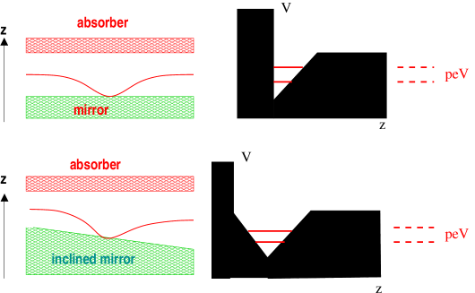
Figure 19: Inclined mirror ensures Parity invariance of QG modifications and hence formalism similar to neutral kaons. A few (two here) energy states (peV energy differences between levels) are inside the Earth’ s potential well.

The neutrons find themselves on a quantum-mechanical potential which is affected by the gravitational potential of Earth, due to their masses. A few energy states, separated by peV $\sim 10^{-15}$ eV energy differences, lie inside the Earth’s potential well. The quantum trajectories of the neutrons are affected by this gravitational potential in the way indicated in the figure. The neutrons are reflected on the mirrors and are collected at the detection point. This has already been demonstrated experimentally, measuring for the first time gravitational effects together with quantum mechanical effects neutrons .

Consider for our purposes the case where two such energy states find themselves inside the potential well. This constitutes a two-level system, and one may think of applying the two-state decoherence formalism to study QG induced effects in such a situation, which would modify the results concering the probabilities of finding the neutrons in one of the two available energy states at the detection point. Like any two-state oscillation system, the respective probabilities should be equal to 1/2 in the absence of any decoherence effects, although in the presence of decoherence one would expect a slight bias in the probabilities.

The quantum number which is conserved here is Parity, which however is the case only if the mirror is inclined, so as to eliminate the effects of parity violation induced by the presence of the Gravitational field. The Probability of finding the neutrons in either state at the detection point indicated in the figure can be computed following the same formalism as the two-state parametrization of the neutral kaon system in ehns , with the replacement of the strangeness conservation by that of parity. The results read, to leading order in the small decoherence parameters:

$${\rm Tr}(\rho^{\prime}\varrho_{1,2})=\frac{1}{2}\pm\frac{1}{2}e^{-\frac{\alpha+\gamma}{2}t}\sin(\Delta Et)~{},\qquad\Delta E={\cal O}({\rm peV})$$ (105)

where $t$ is the time.

We next remark that, if Lorentz invariance is violated by Quantum Gravity, then the decoherence parameters $\alpha,\gamma\simeq\frac{E^{2}_{\rm kin}}{M_{P}}$, where $E_{\rm kin}={\cal O}({\rm peV})$ is the kinetic energy of the neutrons. This is too small to be detected in this kind of experiment; However, in case QG decoherence respects Lorentz Symmetry, which as mentioned above is possible mill ; discr , then $\alpha,\gamma\simeq\frac{m_{n}^{2}}{M_{P}}$. For the duration of the experiment, which is or order $t\sim{\rm msec}$, then, we observe that the decoherence effects are much larger. However, at present, there seems to be no significant sensitivity from this type of experiment, as compared with other available tests of decoherence. Nevertheless, one cannot exclude the possibility of a significant improvement in sensitivity in similar experiments in the foreseeable future, and this is the reason why I included this case briefly in the present set of lectures.

3.14 CPTV through QG Decoherence for Neutrinos: the most sensitive probe to date

Two-generation models

We now come to discuss quantum-gravity decoherence in neutrinos, whose sensitivity in this respect is far more superior than that of neutral kaons, assuming of course a universal nature of QG. This latter assumption, though, requires some second thoughts, given that, as mentioned above, there are theoretical models of quantum space-time foamsynchro , in which QG effects interact differently with various particle species.

With this in mind we next remark that, QG may induce oscillations between neutrino flavours independently of $\nu$-masses liu ; lisi ; benatti ; klapdor . We begin with the simplified case of two-neutrino generations, that is a two-state system, which makes the formalism very similar to the neutral kaon case described above. In similar spirit to the Kaon case, the energy (physical) eigenstates of neutrinos are not flavour eigenstates, and one has mixing.

The basic formalism for decoherence-induced neutrino oscillations is described by a QMV evolution for the density matrix of the $\nu$, which parallels that of neutral kaon in the case of two generations of neutrinos:

$$\partial_{t}\rho=i[\rho,H]+\delta H\hskip-8.5pt/\hskip 2.0pt\rho$$ (106)

where ehns

$${\delta H\hskip-8.5pt/\hskip 2.0pt}_{\alpha\beta}=\left(\begin{array}[]{cccc}0&0&0&0\\ 0&-2\alpha&-2\beta&0\\ 0&-2\beta&-2\gamma&0\\ 0&0&0&0\end{array}\right)$$

for energy and lepton number conservation, and

$${\delta H\hskip-8.5pt/\hskip 2.0pt}_{\alpha\beta}=\left(\begin{array}[]{cccc}0&0&0&0\\ 0&0&0&0\\ 0&0&-2\alpha&-2\beta\\ 0&0&-2\beta&-2\gamma\end{array}\right)$$

if energy and lepton number are violated, but flavour is conserved (the latter associated formally with the $\sigma_{1}$ Pauli matrix).

Positivity of $\rho$, but not complete positivity, requires: $\alpha,\gamma>0,\qquad\alpha\gamma>\beta^{2}$. The parameters $\alpha,\beta,\gamma$ violate CP, and CPT in general, as discussed previously.

The relevant oscillation probabilities, describing the evolution of a neutrino flavour $\nu_{\alpha}$ , created at time $t=0$, to a neutrino flavour $\nu_{\beta}$ at time $t$, are determined by means of the dynamical semigroup approach (32):

$$P_{\nu_{\alpha}\rightarrow\nu_{\beta}}(t)={\rm Tr}\left(\rho_{\alpha}(t)\rho^{\beta}\right)$$ (107)

For our problem we have a two state system, and the computation of the eigenvalue problem is easy. For the two cases above, we obtain after some straightforward algebra liu :

(A) For the flavour conserving case:

As a simplified example, consider the oscillation $\nu_{e}\rightarrow\nu_{x}$  ($x=\mu,\tau$ or sterile):

$$P_{\nu_{e}\rightarrow\nu_{x}}=\frac{1}{2}-\frac{1}{2}e^{-\gamma L}{\rm cos}^{2}2\theta_{v}-\frac{1}{2}e^{-\alpha L}{\rm sin}^{2}2\theta_{v}{\rm cos}(\frac{|m_{\nu_{1}}^{2}-m_{\nu_{2}}^{2}|}{2E_{\nu}}L)$$ (108)

Here $L$ is the oscillation length and $\theta_{v}$ the mixing angle.

In the mass basis one has: $|\nu_{e}>={\rm cos}\theta_{v}|\nu_{1}>+{\rm sin}\theta_{v}|\nu_{2}>,$ $|\nu_{\mu}>=-{\rm sin}\theta_{v}|\nu_{1}>+{\rm cos}\theta_{v}|\nu_{2}>.$ Note that in this case the mixing angle $\theta_{v}=0$ if and only if the neutrinos are massless. From the above considerations, however, it is clear that there are flavour oscillations even in the massless case, due to a non-trivial QG parameter $\gamma$, compatible with flavour conserving formalism: $<\nu_{e}|\sigma_{1}|\nu_{e}>=-<\nu_{\mu}|\sigma_{1}|\nu_{\mu}>=2{\rm sin}\theta_{v}{\rm cos}\theta_{v}.$

(B) For Energy and Lepton number conserving case:

Again, we consider a two-flavour example: $\nu_{e}\rightarrow\nu_{x}$  ($x=\mu,\tau$ or sterile). The relevant oscillation probability in this case is calculated to be liu :

$$P_{\nu_{e}\rightarrow\nu_{x}}=\frac{1}{2}{\rm sin}^{2}2\theta_{v}\left(1-e^{-(\alpha+\gamma)L}{\rm cos}(\frac{|m_{\nu_{1}}^{2}-m_{\nu_{2}}^{2}|}{2E_{\nu}}L)\right)$$ (109)

where we assumed for simplicity, and illustrative purposes, that $\alpha,\beta,\gamma\ll\frac{|m_{\nu_{1}}^{2}-m_{\nu_{2}}^{2}|}{2E_{\nu}}$. The reader is invited to contrast this result with case (A) above.

One can use the results in the cases (A) and (B) to bound experimentally $\xi\equiv\{\alpha,\beta,\gamma$}. At this stage the reader is invited to recall that there exist two kinds of theoretical estimates/predictions for the order of magnitude of the parameters $\alpha,\beta,\gamma$: An optimistic one emn , according to which $\xi\sim\xi_{0}(\frac{E}{\rm GeV})^{n},n=0,2,-1$, and this has a chance of being falsified in future experiments, if the effect is there, and a pessimistic one adler , which depends on the square of the neutrino mass-squared difference (24), $\xi\sim\frac{(\Delta m^{2})^{2}}{E^{2}M_{qg}}$, ($M_{qg}\sim M_{P}\sim 10^{19}$ GeV), which is much smaller, and probably cannot be accessed by immediate future neutrino oscillation experiments.

We now mention that in some models of QG-induced decoherence, complete positivity of $\rho(t)$ for composite systems, such as $\phi$ or $B$ mesons, may be imposed benatti (however, I must stress once more that the necessity of this requirement, especially in a QG context where non-linear effects may be present emn , remains to be proven). This results in an ideal Markov environment, with: $\alpha=\beta=0,\gamma>0$.

If this model is assumed for $\nu$ oscillations induced by QG decoherence lisi , then the following phenomenological parametrization can be made: $\gamma=\gamma_{0}(E/{\rm GeV})^{n}$, $n=0,2,-1$. with $E$ the neutrino energy.

Figure 20: Effects of decoherence ($\gamma=\gamma_{0}={\rm const}\neq 0$) on the distributions of lepton events as a function of the zenith angle $\vartheta$.

Figure 21: Best-fit scenarios for pure oscillations ($\gamma=0$) (solid line) and for pure decoherence with $\gamma\propto 1/E$ (dashed line).

From Atmospheric $\nu$ data one is led to the following bounds for the QG-decoherence parameter $\gamma$ (c.f. figures 20,21) lisi :

(a) $n=0$, $\gamma_{0}<3.5\times 10^{-23}$ GeV.

(b) $n=2$, $\gamma_{0}<0.9\times 10^{-27}$ GeV.

(c) $n=-1$, $\gamma_{0}<2\times 10^{-21}$ GeV.

Especially with respect to case (b) the reader is reminded that the CPLEAR bound on $\gamma$ for neutral Kaons was $\gamma<10^{-21}$ GeV cplear , i.e. the $\nu$-oscillation experiments exhibit much higher sensitivity to QG decoherence effects than neutral meson experiments.

Finally, I note that in klapdor it was remarked that very stringent bounds on $\alpha,\beta$ and $\gamma$ (in the lepton number violating QG case) may be imposed by looking at oscillations of neutrinos from astrophysical sources (supernovae and AGN). The corresponding bounds on the $\gamma$ parameter from oscillation analysis of neutrinos from supernovae and AGN, if QG induces such oscillations, are very strong: $\gamma<10^{-40}$ GeV from Supernova1987a, using the observed constraint sncons on the oscillation probability $P_{\nu_{e}\rightarrow\nu_{\mu},\tau}<0.2$, and $\gamma<10^{-42}$ GeV from AGN, which exhibit sensitivity to order higher than $E^{3}/M_{qg}^{2}$, with $M_{qg}\sim M_{P}\sim 10^{19}$ GeV! Of course, the bounds from AGN do not correspond to real bounds, awaiting the observation of high energy neutrinos from such astrophysical sources. In klapdor bounds have also been derived for the QG decoherence parameters by assuming that QG may induce neutrinoless double-beta decay. However, using current experimental constraints on neutrinoless double-beta decay observables klapdor2 one arrives at very weak bounds for the parameters $\alpha,\beta,\gamma$.

One also expects stringent bounds on decoherence parameters, but also on deformed dispersion relations, if any, for neutrinos, from future underwater neutrino telescopes, such as ANTARES antares , and NESTOR nestor  .

Three-Generation Models: Decoherence and the LSND Result

As we discussed above, two-generation CPTV mass models for neutrinos within quantum mechanics are excluded by global fits of available data, especially solar neutrino models. This situation is not expected to change by the inclusion of a third generation, although I must stress that, as far as I am aware of, complete three-generations analyses of this kind have not been performed as yet. Moreover, although four generation CPTV neutrino models are still consistent with experimental data, nevertheless there seems to be no experimental evidence for a forth generation, especially after the recent WMAP astrophysical results. On the other hand, as we have just seen, two-generation neutrino analysis of decoherence effects did not show any spectacular results, apart from the imposition of stringent bounds on the relevant parameters.

This prompts one to think that the extension of the decoherence formalism to three generations of neutrinos, which from a mathematical view point is a problem with considerable increase in technical complexity, is a futile task, with no physical importance whatsoever. However, there are the “anomalous” results provided by the LSND collaboration lsnd on the evidence for ${\overline{\nu}_{e}}\rightarrow{\overline{\nu}_{\mu}}$ oscillations, through ${\overline{\nu}_{e}}$ disappearance, but not for the cooresponding oscillations in the neutrino sector, which call for an explanation, if one, of course, takes them seriously into account. These effects, as we have seen, cannot be explained by conventional quantum field theoretic analyses, even if CPT is assumed violated.

It is the point of this subsection to point out that, if one extends the decoherence analysis to three generations of neutrinos and allows for CPT Violation among the decoherence parameters, it is possiblebm to fit all the currently availble neutrino data, including the LSND results, by simple decoherence models, in which the dominant decoherence parameters occur in the antineutrino sector. It is important that in such “asymmetric” decoherence models there is no need for enlarging the neutrino sector by a fourth generation, neither for introducing CPTV mass parameters. If the LSND results are confirmed by future experiments, then this would be a significant result, as it would provide for the first time a clear experimental evidence for a CPTV decoherence event, which would be directly related to quantum gravity effects.

Let us briefly present the arguments leading to these results. Formally, the extension of the completely positive decoherence scenario to the standard three-generation neutrino oscillations case is straightforward, and it was described in section two. One adopts a three-state Lindblad problem, and, following the standard procedure outlined there, one determines the corresponding eigenvectors and eigenvalues, as in the two-level case examined in the previous subsection. It is only a considerable increase in mathematical complexity, and obscurity in the precise physical meaning of all the non-trivial entries of the decoherence matrix that one encounters here.

The relativistic neutrino Hamiltonian $H_{\rm eff}\sim p^{2}+m^{2}/2p$, with $m$ the neutrino mass, is used as the effective Hamiltonian of the subsystem in the evolution equation (14). In terms of the generators ${\cal J}_{\mu}$, $\mu=0,\dots 8$ of the SU(3) group, $H_{\rm eff}$ can be expanded as gago : ${\cal H}_{\rm eff}=\frac{1}{2p}\sqrt{2/3}\left(6p^{2}+\sum_{i=1}^{3}m_{i}^{2}\right){\cal J}_{0}+\frac{1}{2p}(\Delta m_{12}^{2}){\cal J}_{3}+\frac{1}{2\sqrt{3}p}\left(\Delta m_{13}^{2}+\Delta m_{23}^{2}\right){\cal J}_{8}$, with the obvious notation $\Delta m_{ij}^{2}=m_{i}^{2}-m_{j}^{2}$, $i,j=1,2,3$.

The analysis of gago assumed ad hoc a diagonal form for the $9\times 9$ decoherence matrix ${\cal L}$ in (27):

$$[{\cal L}_{\mu\nu}]={\rm Diag}\left(0,-\gamma_{1},-\gamma_{2},-\gamma_{3},-\gamma_{4},-\gamma_{5},-\gamma_{6},-\gamma_{7},-\gamma_{8}\right)$$ (110)

in direct analogy with the two-level case of complete positivity lisi ; benatti . As we have mentioned already, there is no strong physical motivation behind such restricted forms of decoherence. This assumption, however, leads to the simplest possible decoherence models, and, for our phenomenological purposes in this work, we will assume the above form, which we will use to fit all the available neutrino data. It must be clear to the reader though, that such a simplification, if proven to be successful (which, as we shall argue below, is the case here), just adds more in favor of decoherence models, given the restricted number of available parameters for the fit in this case. In fact, any other non-minimal scenario will have it easier to accommodate data because it will have more degrees of freedom available for such a purpose.

Specifically we shall look at transition probabilities (107), which can be computed in a straightforward manner within the dynamical-semigroups approach outlined previously gago :

$$P(\nu_{\alpha}\rightarrow\nu_{\beta})={\rm Tr}[\rho^{\alpha}(t)\rho^{\beta}]=$$

$$\frac{1}{3}+\frac{1}{2}\sum_{i,k,j}e^{\lambda_{k}t}{\cal D}_{ik}{\cal D}_{kj}^{-1}\rho^{\alpha}_{j}(0)\rho_{i}^{\beta}$$ (111)

where $\alpha,\beta=e,\mu,\tau$ stand for the three neutrino flavors, and Latin indices run over $1,\dots 8$. The quantities $\lambda_{k}$ are the eigenvalues of the matrix ${\cal M}$ appearing in the evolution (27), after taking into account probability conservation, which decouples $\rho_{0}(t)=\sqrt{2/3}$, leaving the remaining equations in the form: $\partial\rho_{k}/\partial t=\sum_{j}{\cal M}_{kj}\rho_{j}$. The matrices ${\cal D}_{ij}$ are the matrices that diagonalize ${\cal M}$ lindblad . Explicit forms of these matrices, the eigenvalues $\lambda_{k}$, and consequently the transition probabilities (111), are given in gago .

The important point to stress is that, in generic models of oscillation plus decoherence, the eigenvalues $\lambda_{k}$ depend on both the decoherence parameters $\gamma_{i}$ and the mass differences $\Delta m^{2}_{ij}$. For instance, $\lambda_{1}=\frac{1}{2}[-(\gamma_{1}+\gamma_{2})-\sqrt{(\gamma_{2}-\gamma_{1})^{2}-4\Delta_{12}^{2}}]$, with the notation $\Delta_{ij}\equiv\Delta m_{ij}^{2}/2p$, $i,j=1,2,3$. Note that, to leading order in the (small) squared-mass differences, one may replace $p$ by the total neutrino energy $E$, and this will be understood in what follows.

We now note that it is a generic feature of the $\lambda_{k}$ to depend on the quantities $\Omega_{ij}$ which are given bybm ; gago

$$\Omega_{12} = \sqrt{(\gamma_{2}-\gamma_{1})^{2}-4\Delta_{12}^{2}}$$

$$\Omega_{13} = \sqrt{(\gamma_{5}-\gamma_{4})^{2}-4\Delta_{13}^{2}}$$

$$\Omega_{23} = \sqrt{(\gamma_{7}-\gamma_{6})^{2}-4\Delta_{23}^{2}}\qquad{\rm etc.}$$ (112)

From the above expressions for the eigenvalues $\lambda_{k}$, it becomes clear that, when decoherence and oscillations are present simultaneously, one should distinguish two cases, according to the relative magnitudes of $\Delta_{ij}$ and $\Delta\gamma_{kl}\equiv\gamma_{k}-\gamma_{l}$: (i) $2|\Delta_{ij}|\geq|\Delta\gamma_{k\ell}|$, and (ii) $2|\Delta_{ij}|<|\Delta\gamma_{k\ell}|$. In the former case, the probabilities (111) contain trigonometric (sine and cosine) functions, whilst in the latter they exhibit hyperbolic sin and cosine dependence.

Assuming mixing between the flavours, amounts to expressing neutrino flavor eigenstates $|\nu_{\alpha}>$, $\alpha=e,\mu,\tau$ in terms of mass eigenstates $|\nu_{i}>$, $i=1,2,3$ through a (unitary) matrix $U$: $|\nu_{\alpha}>=\sum_{i=1}^{3}U^{*}_{\alpha i}|\nu_{i}>$. This implies that the density matrix of a flavor state $\rho^{\alpha}$ can be expressed in terms of mass eigenstates as: $\rho^{\alpha}=|\nu_{\alpha}><\nu_{\alpha}|=\sum_{i,j}U^{*}_{\alpha i}U_{\alpha j}|\nu_{i}><\nu_{j}|$. From this we can determine $\rho_{\mu}^{\alpha}=2{\rm Tr}(\rho^{\alpha}{\cal J}_{\mu})$, a quantity needed to calculate the transition probabilities (111).

The important comment bm we would like to raise at this point is that, when considering the above probabilities in the antineutrino sector, the respective decoherence parameters ${\bar{\gamma}}_{i}$ in general may be different from the corresponding ones in the neutrino sector, as a result of the strong form of CPT violation. In fact, as we shall discuss next, this will be crucial for accommodating the LSND result without conflicting with the rest of the available neutrino data. This feature is totally unrelated to mass differences between flavors.

In gago a pessimistic conclusion was drawn on the “clear incompatibility between neutrino data and theoretical expectations”, as followed by their qualitative tests for decoherence. It is a key feature of the work of bm to point out that this point of view may not be true at all. In fact, as we shall demonstrate below, if one takes into account all the available neutrino data, including the final LSND results lsnd , which the authors of gago did not do, and allows for the above mentioned CPT violation in the decoherence sector, then one will arrive at exactly the opposite conclusion, namely that three-generation decoherence and oscillations can fit the data successfully!

As shown in bm , compatibility of all available data, including CHOOZ chooz and LSND, can be achieved through a set of decoherence parameters $\gamma_{j}$ with energy dependences $\gamma^{0}_{j}E$ and $\gamma^{0}_{j}/E$, with $\gamma^{0}_{j}\sim 10^{-18},10^{-24}$ (GeV)², respectively, for some $j$’s, and in fact the fit ends up being significantly better than the standard one (when LSND results are included) as evidenced by an appropriate $\chi^{2}$ analysis.

Some important remarks are in order. First of all, in the analysis of gago pure decoherence is excluded in three-generation scenaria, as in two generation ones, due to the fact that the transition probabilities in the case $\Delta m_{ij}^{2}=0$ (pure decoherence) are such that the survival probabilities in both sectors are equal, i.e. $P(\nu_{\alpha}\rightarrow\nu_{\alpha})=P({\overline{\nu}}_{\alpha}\rightarrow{\overline{\nu}}_{\alpha})$. From (111) we have in this case gago :

$$P_{\nu_{e}\rightarrow\nu_{e}}=P_{\nu_{\mu}\rightarrow\nu_{\mu}}\simeq\frac{1}{3}+\frac{1}{2}e^{-\gamma_{3}t}+\frac{1}{6}e^{-\gamma_{8}t}$$ (113)

From the CHOOZ experiment chooz , for which $L/E\sim 10^{3}/3$ m/MeV, we have that $\langle P_{{\bar{\nu}}_{e}\rightarrow{\bar{\nu}}_{e}}\rangle\simeq 1$, while the K2K experiment K2K with $L/E\sim 250/1.3$  km/GeV has observed events compatible with $\langle P_{\nu_{\mu}\rightarrow\nu_{\mu}}\rangle\simeq 0.7$, thereby contradicting the theoretical predictions (113) of pure decoherence.

However, this conclusion is based on the fact that in the antineutrino sector the decoherence matrix is the same as that in the neutrino sector. In general this need not be the case, in view of CPT Violation, which could imply a different interaction of the antiparticle with the gravitational environment as compared with the particle. In fact in models where a pure state evolves to a mixed one, one expects a CPT Violation in the strong form, according to the theorem of wald .

In our tests we took into account this possibility, but pure decoherence can be excluded also in this case, as it is clearly incompatible with the totality of the available data.

In order to check our model, we have performed a $\chi^{2}$ comparison (as opposed to a $\chi^{2}$ fit which is still pending) to SuperKamiokande sub-GeV and multi GeV data, CHOOZ data and LSND, for a sample point in the vast parameter space of our extremely simplified version of decoherence models. Since we have not performed as yet a $\chi^{2}$-fit, the point we are selecting (rather visually and not by a proper $\chi^{2}$ analysis) is not optimized to give the best fit to the existing data. Instead, it must be regarded as one among the many equally good members in this family of solutions, being extremely possible to find another model that fits better the data, through a complete (and highly time consuming) scan over the whole parameter space.

Cutting the long story short, and to make the analysis easier, we have setbm all the $\gamma_{i}$ in the neutrino sector to zero, restricting in this way all the dominant decoherence effects in the antineutrino sector only. For the sake of simplicity we have assumed the form:

$$\bar{\gamma}_{i}=\bar{\gamma}_{i+1}~{}{\rm for}~{}~{}i=1,4,6\qquad{\rm and}\qquad\bar{\gamma}_{3}=\bar{\gamma}_{8}$$ (114)

Later on we shall set some of the $\gamma_{i}$’s to zero. Furthermore, we have also set the CP violating phase of the NMS matrix to zero, so that all the mixing matrix elements become real.

With these assumptions, the otherwise cumbersome expression (see end of section for more detailed results) for the transition probability for the antineutrino sector takes the form:

$$P_{\bar{\nu}_{\alpha}\rightarrow\bar{\nu}_{\beta}} = \frac{1}{3}+\frac{1}{2}\left\{\rho_{1}^{\alpha}\rho_{1}^{\beta}\cos\left(\frac{|\Omega_{12}|t}{2}\right)e^{-\bar{\gamma}_{1}t}\right.$$ (115)

$$+ \rho_{4}^{\alpha}\rho_{4}^{\beta}\cos\left(\frac{|\Omega_{13}|t}{2}\right)e^{-\bar{\gamma}_{4}t}$$

$$+ \rho_{6}^{\alpha}\rho_{6}^{\beta}\cos\left(\frac{|\Omega_{23}|t}{2}\right)e^{-\bar{\gamma}_{6}t}$$

$$+ e^{-\bar{\gamma}_{3}t}\left(\rho_{3}^{\alpha}\rho_{3}^{\beta}+\rho_{8}^{\alpha}\rho_{8}^{\beta}\right)\Bigg{\}}.$$

where the $\Omega_{ij}$ were defined in the previous section and are the same in both sectors (due to our choice of $\gamma_{i}$’s) and

$$\rho^{\alpha}_{0} = \sqrt{\frac{2}{3}}$$

$$\rho^{\alpha}_{1} = 2Re(U_{\alpha 1}^{*}U_{\alpha 2})$$

$$\rho^{\alpha}_{2} = -2Im(U_{\alpha 1}^{*}U_{\alpha 2})$$

$$\rho^{\alpha}_{3} = |U_{\alpha 1}|^{2}-|U_{\alpha 2}|^{2}$$

$$\rho^{\alpha}_{4} = 2Re(U_{\alpha 1}^{*}U_{\alpha 3})$$

$$\rho^{\alpha}_{5} = -2Im(U_{\alpha 1}^{*}U_{\alpha 3})$$

$$\rho^{\alpha}_{6} = 2Re(U_{\alpha 2}^{*}U_{\alpha 3})$$

$$\rho^{\alpha}_{7} = -2Im(U_{\alpha 2}^{*}U_{\alpha 3})$$

$$\rho^{\alpha}_{8} = \sqrt{\frac{1}{3}}\left(|U_{\alpha 1}|^{2}+|U_{\alpha 2}|^{2}-2|U_{\alpha 3}|^{2}\right)$$ (116)

where the mixing matrices are the same as in the neutrino sector. For the neutrino sector, as there are no dominant decoherence effects, the standard expression for the transition probability is valid.

It is obvious now that, since the neutrino sector does not suffer from decoherence, there is no need to include the solar data into the fit. We are guaranteed to have an excellent agreement with solar data, as long as we keep the relevant mass difference and mixing angle within the LMA region. As mentioned previously, CPT violation is driven by, and restricted to, the decoherence parameters, and hence masses and mixing angles are the same in both sectors, and selected to be

$\Delta m_{12}^{2}=\Delta\overline{m_{12}}^{2}=7\cdot 10^{-5}$ eV²,

$\Delta m_{23}^{2}=\Delta\overline{m_{23}}^{2}=2.5\cdot 10^{-3}$ eV²,

$\theta_{23}=\overline{\theta_{23}}=\pi/4$, $\theta_{12}=\overline{\theta_{12}}=.45$,

$\theta_{13}=\overline{\theta_{13}}=.05$,

as indicated by the state of the art phenomenological analysis in neutrino physics.

For the decoherence parameters we have chosen (c.f. (114))

$$\overline{\gamma_{1}}=\overline{\gamma_{2}}=2\cdot 10^{-18}\cdot E~{}~{}{\rm and}~{}~{}\overline{\gamma_{3}}=\overline{\gamma_{8}}=1\cdot 10^{-24}/E~{},$$ (117)

where $E$ is the neutrino energy, and barred quantities refer to the antineutrinos, given that decoherence takes place only in this sector in our model. All the other parameters are assumed to be zero. All in all, we have introduced only two new parameters, two new degrees of freedom, $\overline{\gamma_{1}}$ and $\overline{\gamma_{3}}$, and we shall try to explain with them all the available experimental data.

In order to test our model with these two decoherence parameters in the antineutrino sector, we have calculated the zenith angle dependence of the ratio “observed/(expected in the no oscillation case)”, for muon and electron atmospheric neutrinos, for the sub-GeV and multi-GeV energy ranges, when mixing is taken into account. The results are shown in Fig. 22. where, for the sake of comparison, we have also included the experimental data.

Figure 22: Decoherence fits, from top to bottom: (a) pure decoherence in antineutrino sector, (b) pure decoherence in both sectors, (c) mixing plus decoherence in the antineutrino sector only, (d) mixing plus decoherence in both sectors. The dots correspond to SK data.

As bare-eye comparisons can be misleading, we have also calculated the $\chi^{2}$ value for each of the cases, defining the atmospheric $\chi^{2}$ as

$$\chi^{2}_{\rm atm}=\sum_{M,S}\sum_{\alpha=e,\mu}\sum_{i=1}^{10}\frac{(R_{\alpha,i}^{\rm exp}-R_{\alpha,i}^{\rm th})^{2}}{\sigma_{\alpha i}^{2}}\quad.$$ (118)

Here $\sigma_{\alpha,i}$ are the statistical errors, the ratios $R_{\alpha,i}$ between the observed and predicted signal can be written as

$$R_{\alpha,i}^{\rm exp}=N_{\alpha,i}^{\rm exp}/N_{\alpha,i}^{\rm MC}$$ (119)

(with $\alpha$ indicating the lepton flavor and $i$ counting the different bins, ten in total) and $M,S$ stand for the multi-GeV and sub-GeV data respectively. For the CHOOZ experiment we used the 15 data points with their statistical errors, where in each bin we averaged the probability over energy and for LSND one datum has been included. The results with which we hope all our claims become crystal clear are summarized in Table 3, were we present the $\chi^{2}$ comparison for the following cases: (a) pure decoherence in the antineutrino sector, (b) pure decoherence in both sectors, (c) mixing plus decoherence in the antineutrino sector, (d) mixing plus decoherence in both sectors, and (e) mixing only - the standard scenario.

model	$\chi^{2}$ without LSND	$\chi^{2}$ including LSND
(a)	980.7	980.8
(b)	979.8	980.0
(c)	52.2	52.3
(d)	54.4	54.6
(e)	53.9	60.7

Table 3: $\chi^{2}$ obtained for (a) pure decoherence in antineutrino sector, (b) pure decoherence in both sectors, (c) mixing plus decoherence in the antineutrino sector only, (d) mixing plus decoherence in both sectors, (e) standard scenario with and without the LSND result.

From the table it becomes clear that the mixing plus decoherence scenario in the antineutrino sector can easily account for all the available experimental information, including LSND data. It is important to stress once more that our sample point was not obtained through a scan over all the parameter space, but by an educated guess, and therefore plenty of room is left for improvements. At this point a word of warning is in order: although superficially it seems that scenario (d), decoherence plus mixing in both sectors, provides an equally good fit, one should remember that including decoherence effects in the neutrino sector can have undesirable effects in solar neutrinos, especially due to the fact that decoherence effects are weighted by the distance traveled by the neutrino, something that may lead to seizable (not observed!) effects in the solar case.

One might wonder then, whether decohering effects, which affect the antineutrino sector sufficiently to account for the LSND result, have any impact on the solar-neutrino related parameters, measured through antineutrinos in the KamLAND experimentkamland . In order to answer this question, it will be sufficient to calculate the electron survival probability for KamLAND in our model, which turns out to be $P_{\bar{\nu}_{\alpha}\rightarrow\bar{\nu}_{\beta}}\mid_{\mbox{\tiny KamLAND}}\simeq.63$, in perfect agreement with observations. It is also interesting to notice that in our model, the LSND effect is not given by the phase inside the oscillation term ( which is proportional to the solar mass difference) but rather by the decoherence factor multiplying the oscillation term. Therefore the tension between LSND and KARMENkarmen data is naturally eliminated, because the difference in length leads to an exponential suppression.

Having said that, it is now clear that decoherence models (once neutrino mixing is taken into account) are the best (and arguably the only) way to explain all the observations including the LSND result. This scenario , which makes dramatic predictions for the upcoming neutrino experiments, expresses a strong observable form of CPT violation in the laboratory, and in this sense, our fit gives a clear answer to the question as to whether the weak form of CPT invariance (11) is violated in Nature. It seems that, in order to account for the LSND results, we should invoke such a decoherence-induced CPT Violation, which however is independent of any mass differences between particles and antiparticles.

This CPT violating pattern, with equal mass spectra for neutrinos and antineutrinos, if true, will have dramatic signatures in future neutrino oscillation experiments. The most striking consequence will be seen in MiniBooNE miniboone , According to our picture, MiniBooNE will be able to confirm LSND only when running in the antineutrino mode and not in the neutrino one, as decoherence effects live only in the former. Smaller but experimentally accessible signatures will be seen also in MINOS minos , by comparing conjugated channels (most noticeably, the muon survival probability).

We next remark that fits with decoherence parameters with energy dependences of the form (117) imply that the exponential factors $e^{\lambda_{k}t}$ in (111) due to decoherence will modify the amplitudes of the oscillatory terms due to mass differences, and while one term depends on $L/E$ the other one is driven by $L\cdot E$, where we have set $t=L$, with $L$ the oscillation length (we are working with natural units where $c=1$).

The order of the coefficients of these quantities, $\gamma^{0}_{j}\sim 10^{-18},10^{-24}$ (GeV)², found in our sample point, implies that for energies of a few GeV, which are typical of the pertinent experiments, such values are not far from $\gamma_{j}^{0}\sim\Delta m_{ij}^{2}$. If our conclusions survive the next round of experiments, and therefore if MiniBOONE experiment miniboone confirms previous LSND claims, then this may be a significant result.

Indeed, one would be tempted to speculate that, if the above estimate holds, and the decoherence coefficients are proportional to the neutrino mass-squared differences, this could even indicate that the neutrino mass differences themselves might be due to quantum gravity decoherence, in the sense of environmental contributions to the effective neutrino Hamiltonian appearing in the decoherent evolution (14), which could mascarade themselves as mass terms. Theoretically it is still unknown how the neutrinos acquire a mass, or what kind of mass (Majorana or Dirac) they possess. There are scenaria in which the mass of neutrino may be due to some peculiar backgrounds of string theory for instance. If the above model turns out to be right we might then have, for the first time in low energy physics, an indication of a direct detection of a quantum gravity effect, which disguised itself as an induced decohering neutrino mass difference. Notice that in our sample point only antineutrinos have non-trivial decoherence parameters $\overline{\gamma_{i}}$ , for $i=1$ and 3, while the corresponding quantities in the neutrino sector vanish. This implies that there is a single cause for mass differences, the decoherence in antineutrino sector, which is compatible with common mass differences in both sectors. This would be very interesting, if true.

Finally, before closing, we would like to remark on extensions of the above phenomenologiocal model for decoherence by including non-diagonal terms in the decoherence matrix $L_{\mu\nu}$. As mentioned above, the physical significance of such extensions is not clear, and indeed it cannot be clear from simple phenomenological analyses like the one presented here. One needs a detailed knoweldge of the QG decoherence effects so as to obtain such an understanding.

Nevertheless one may test the phenomenological efficiency of the simple parametrisation of gago ; bm by comparing the results on the oscillation probabilities versus models where off diagonal terms are included in the decoherence matrix. As a simple example, consider the following form of the decoherence matrix waldron :

$${\cal M}=\left(\begin{array}[]{cccccccc}L_{11}&-\Delta_{12}+L_{12}&0&0&0&0&0&0\\ \Delta_{12}+L_{12}&L_{22}&0&0&0&0&0&0\\ 0&0&L_{33}&0&0&0&0&0\\ 0&0&0&L_{44}&-\Delta_{13}+L_{45}&0&0&0\\ 0&0&0&\Delta_{13}+L_{45}&L_{55}&0&0&0\\ 0&0&0&0&0&L_{66}&-\Delta_{23}+L_{67}&0\\ 0&0&0&0&0&\Delta_{23}+L_{67}&L_{77}&0\\ 0&0&0&0&0&0&0&L_{88}\\ \end{array}\right)$$

(128)

where ${\cal M}$ is the matrix appearing in the decoherent evolution (31). It is again a straightforward but tedious exercise to determine the matrix which diagonalises ${\cal M}$ and find the eigenvalues and eigenvectors of ${\cal M}$, which determine the oscillation probabilities (111). Defining $\Gamma_{ij}$ as

$$\Gamma_{12}\equiv\sqrt{(L_{11}-L_{22})^{2}+4L_{12}^{2}-4\Delta_{12}^{2}}$$ (129)

and similarly for the other elements, and taking notice of the fact that $\Gamma_{ij}$ are similar to the $\Omega_{ij}$ of the diagonal decoherence case (112), with the only difference being an extra positive term ($L_{12}^{2}$ etc.) under the sqare root, we can compute the corresponding oscillation probabilities (111). For completeness we give here the relevant expression, which allows the interested reader to derive the diagonal case expressions by setting the off-digonal elements of $L_{\mu\nu}$ equal to zero. We have:

$$P_{\nu_{\alpha}\rightarrow\nu_{\beta}}(t)=\frac{1}{3}+\frac{1}{2}e^{\frac{(L_{11}+L_{22})t}{2}}\left\{\left(\rho_{1}^{\alpha}\rho_{1}^{\beta}+\rho_{2}^{\alpha}\rho_{2}^{\beta}\right)\left(\frac{e^{\frac{\Gamma_{12}t}{2}}+e^{-\frac{\Gamma_{12}t}{2}}}{2}\right)\right.\qquad\qquad\qquad\qquad\qquad\qquad$$

$$\left.+\left[\left(\rho_{1}^{\alpha}\rho_{1}^{\beta}-\rho_{2}^{\alpha}\rho_{2}^{\beta}\right)\left(\frac{L_{11}-L_{22}}{\Gamma_{12}}\right)+\frac{2\rho_{2}^{\alpha}\rho_{1}^{\beta}(-L_{12}+\Delta_{12})-2\rho_{1}^{\alpha}\rho_{2}^{\beta}(L_{12}+\Delta_{12})}{\Gamma_{12}}\right]\left(\frac{e^{\frac{\Gamma_{12}t}{2}}-e^{-\frac{\Gamma_{12}t}{2}}}{2}\right)\right\}$$

$$+e^{\frac{(L_{44}+L_{55})t}{2}}\left\{\left(\rho_{4}^{\alpha}\rho_{4}^{\beta}+\rho_{5}^{\alpha}\rho_{5}^{\beta}\right)\left(\frac{e^{\frac{\Gamma_{13}t}{2}}+e^{-\frac{\Gamma_{13}t}{2}}}{2}\right)\right.\qquad\qquad\qquad\qquad\qquad\qquad$$

$$\left.+\left[\left(\rho_{4}^{\alpha}\rho_{4}^{\beta}-\rho_{5}^{\alpha}\rho_{5}^{\beta}\right)\left(\frac{L_{44}-L_{55}}{\Gamma_{13}}\right)+\frac{2\rho_{5}^{\alpha}\rho_{4}^{\beta}(-L_{45}+\Delta_{13})-2\rho_{4}^{\alpha}\rho_{5}^{\beta}(L_{45}+\Delta_{13})}{\Gamma_{13}}\right]\left(\frac{e^{\frac{\Gamma_{13}t}{2}}-e^{-\frac{\Gamma_{13}t}{2}}}{2}\right)\right\}$$

$$+e^{\frac{(L_{66}+L_{77})t}{2}}\left\{\left(\rho_{6}^{\alpha}\rho_{6}^{\beta}+\rho_{7}^{\alpha}\rho_{7}^{\beta}\right)\left(\frac{e^{\frac{\Gamma_{23}t}{2}}+e^{-\frac{\Gamma_{23}t}{2}}}{2}\right)\right.\qquad\qquad\qquad\qquad\qquad\qquad$$

$$\left.+\left[\left(\rho_{6}^{\alpha}\rho_{6}^{\beta}-\rho_{7}^{\alpha}\rho_{7}^{\beta}\right)\left(\frac{L_{66}-L_{77}}{\Gamma_{23}}\right)+\frac{2\rho_{7}^{\alpha}\rho_{6}^{\beta}(-L_{67}+\Delta_{23})-2\rho_{6}^{\alpha}\rho_{7}^{\beta}(L_{67}+\Delta_{23})}{\Gamma_{23}}\right]\left(\frac{e^{\frac{\Gamma_{23}t}{2}}-e^{-\frac{\Gamma_{23}t}{2}}}{2}\right)\right\}$$

$$+e^{L_{33}t}\rho_{3}^{\alpha}\rho_{3}^{\beta}+e^{L_{88}t}\rho_{8}^{\alpha}\rho_{8}^{\beta}\qquad\qquad\qquad\qquad\qquad\qquad\qquad\qquad\qquad\qquad\qquad\qquad$$ (130)

Assuming $\Gamma_{ij}$ to be imaginary, as in the diagonal case, taking $\sin\left(\frac{|\Gamma_{ij}|t}{2}\right)\approx 0$, and recalling (3.14), we observe that, with real values for the elements of the mixing matrix U, one obtains the same form for the oscillation probability as in bm , provided the choice (117) is made for the diagonal elements:

$$P_{\nu_{\alpha}\rightarrow\nu_{\beta}}(t)=\frac{1}{3}+\frac{1}{2}e^{\frac{(L_{11}+L_{22})}{2}}\left(\rho_{1}^{\alpha}\rho_{1}^{\beta}\right)\cos\left(\frac{|\Gamma_{12}|t}{2}\right)$$

$$+e^{\frac{(L_{44}+L_{55})}{2}}\left(\rho_{4}^{\alpha}\rho_{4}^{\beta}\right)\cos\left(\frac{|\Gamma_{13}|t}{2}\right)$$

$$+e^{\frac{(L_{66}+L_{77})}{2}}\left(\rho_{6}^{\alpha}\rho_{6}^{\beta}\right)\cos\left(\frac{|\Gamma_{23}|t}{2}\right)$$

$$e^{L_{33}t}\rho_{3}^{\alpha}\rho_{3}^{\beta}+e^{L_{88}t}\rho_{8}^{\alpha}\rho_{8}^{\beta}$$ (131)

the difference being that $\Gamma_{ij}$, as noted earlier (129), is of a slightly different form from the respective $\Omega_{ij}$ (112), due to the presence of the off-diagonal elements $L_{12}\neq 0$ etc.. Notice from (129) that there is a tendency of the off diagonal elements of the decoherence matrix to reduce the effects of the neutrino mass squared difference $\Delta_{ij}^{2}$ Thus, this sort of extension beyond the diagonal form of the decoherence matrix (110) will affect the magnitude of the oscillation length, as compared to the diagonal case.

It is straightforward to use such parametrizations to obtain bounds on the extra decoherence parameters by comparison with data. We stress again, that, due to CPT Violation, the above probabilities may differ between particles and antiparticles sectors insofar as the order of magnitude of the corresponding decoherence parameters is concerned. Moreover, in view of our comments above on the possible contributions of a decohering environment to the Hamiltonian terms in (14), it is also of great theoretical and phenomenological interest to consider the case of modified dispersion relations for neutrinos simultaneously with the above-described decoherence effects, and compare with current experimental limits. Such modifications may indeed have a common origin with the decohering effects, the interactions with the space time foam. In view of the effects (129) on the oscillation length, analyses like the one in eichler , bounding the coefficients of modified dispersion relations by means of their effects on neutrino oscillations, need therefore to be rethought.

4 Conclusions

In these lectures I discussed various theoretical ideas and phenomenological tests of possible CPT Violation induced by quantum gravity. From this exposition it becomes clear, I hope, that CPT Violation may not be an academic issue, and indeed it may characterize a natural theory of quantum gravity.

There are several probes of CPT Violation and there is no single figure of merit for it. Neutrinos seem to provide the most stringent constraints on CPT Violation through quantum decoherence to date, which in some cases are much stronger than constraints from neutral meson experiments and factories. In this sense neutrinos may provide a very useful guide in our quest for a theory of Quantum Gravity.

Neutrino oscillation experiments provide stringent bounds on many quantum gravity models entailing Lorentz Invariance Violation. There are also plenty of low energy nuclear and atomic physics experiments which yield stringent bounds in models with Lorentz (LV) and CPT Violation (notice that the frame dependence of LV effects is crucial for such high sensitivities). It is my firm opinion that neutrino factories, when built, will undoubtedly shed light on such important and fundamental issues and provide definitive answers to many questions related to LV models of quantum space time.

However, as I repeatedly stressed during these lectures, Quantum Gravity may exhibit Lorentz Invariant (and hence frame independent) CPTV Decoherence. Theoretically, the presence of an environment may be consistent with Lorentz Invariance. This scenario is still compatible with all the existing $\nu$ data, including LSND “anomalous” results, within three generation models, and without the need for introducing matter-antimatter mass differences. Of course the order of the decoherence parameters of such models is highly model dependent, and, hence, at present it is the experiment that may guide the theory insofar as properties and estimates of QG decoherence effects are concerned. It is interesting to remark that, in cases where quantum gravity induces neutrino oscillations between flavours or violates lepton number, the sensitivity of experiments looking for astrophysical neutrinos from extragalactic sources may exceed the order of $1/M_{P}^{2}$ in the respective figures of merit, and thus is far more superior than the sensitivities of meson factories and nuclear and atomic physics experiments as probes of quantum mechanics.

However, as I remarked previously, the reader should be alert to the fact that there is no single figure of merit for CPT Violation; thus, as we have seen, there may be novel CPTV effects unrelated, in principle, to LV and locality violations, which are associated with modifications of EPR correlations. Such effects may be inapplicable to neutrinos, and thus testable only in meson factories or other situations involving entangled states, e.g. in quantum optics.

Clearly much more work, both theoretical and experimental, is needed before definite conclusions are reached on this important research topic, called phenomenology and theory of CPT Violation. I personally believe that this issue lies at the heart of a complete and realistic theory of quantum gravity. For instance, CPT and its Violation is certainly an issue associated with DSR theories, discussed in this School, and non-commutative geometries, which we did not discuss here, but which, as I mentioned in the beginning of the lectures, is also a very active and rich field of research towards a theory of quantum gravity.

In this respect, I believe firmly that theoretical and phenomenological research on sensitive probes of CPT and quantum mechanics, such as photons from extraglactic sources, neutrinos and neutral mesons, could soon make important contributions to our fundamental quest for understanding the quantum structure of space time. Neutrino research certainly constitutes a very interesting and rapidly developing area of fundamental physics, which already provides fruitful collaboration between astrophysics and particle physics, and which, apart from the exciting results on non-zero neutrino masses which has yielded so far, may still hide even further surprises waiting to be discovered in the near future. But other probes, such as photons and neutral mesons, may also prove invaluable in this respect, especially if QG effects discriminate between particle species, a possibility, which as I mentioned in these lectures, may not be so unrealistic.

Let me close, therefore, these lectures with the wish that by the year 2015, when the physics community will be summoned to celebrate the centennial from the development of General Relativity, the dynamical theory of curved space-time geometries, we shall have obtained some concrete experimental indications on what is going on in Physics near the Planck scale. Let us sincerely hope that this exciting prospect will not remain only a wish for the years to come.

References

- (1) M. B. Green, J. H. Schwarz and E. Witten, Superstring Theory. Vols. 1 & 2 (Cambridge University Press 1987); J. Polchinski, String Theory. Vols. 1 & 2(Cambridge University Press 1998). See also, E. Alvarez, lectures in this School.
- (2) J. Ellis, N.E. Mavromatos and D.V. Nanopoulos, Phys. Lett. B293 (1992) 37; J. Chaos, Solitons and Fractals 10, 345 (eds. C. Castro and M.S. El Naschie, Elsevier Science, Pergamon 1999) [hep-th/9805120], and references therein.
- (3) see for instance L. Smolin, arXiv:hep-th/0303185, and references therein.
- (4) L. Smolin, Lectures in this volume.
- (5) See presentation by J. Lukierski, this School and references therein.
- (6) J. Kowalski-Glikman, lectures in this School, and references therein.
- (7) G. Amelino-Camelia, J. R. Ellis, N. E. Mavromatos and D. V. Nanopoulos, Int. J. Mod. Phys. A 12 (1997) 607 [arXiv:hep-th/9605211].
- (8) J. R. Ellis, N. E. Mavromatos and A. S. Sakharov, Astropart. Phys. 20 (2004) 669 [arXiv:astro-ph/0308403]. J. R. Ellis, N. E. Mavromatos, D. V. Nanopoulos and A. S. Sakharov, Nature, Brief Comm. in press [arXiv:gr-qc/0312044]; J. R. Ellis, N. E. Mavromatos and M. Westmuckett, arXiv:gr-qc/0405066.
- (9) J. R. Ellis, N. E. Mavromatos and D. V. Nanopoulos, Phys. Rev. D 62 (2000) 084019 [arXiv:gr-qc/0006004].
- (10) G. Amelino-Camelia, J. R. Ellis, N. E. Mavromatos and D. V. Nanopoulos, Int. J. Mod. Phys. A12 (1997) 607 [arXiv:hep-th/9605211]; G. Amelino-Camelia, J. R. Ellis, N. E. Mavromatos, D. V. Nanopoulos and S. Sarkar, Nature 393 (1998) 763 [arXiv:astro-ph/9712103].
- (11) J. R. Ellis, K. Farakos, N. E. Mavromatos, V. A. Mitsou and D. V. Nanopoulos, Astrophys. J. 535 (2000) 139 [arXiv:astro-ph/9907340]; J. R. Ellis, N. E. Mavromatos, D. V. Nanopoulos and A. S. Sakharov, Astron. Astrophys. 402 (2003) 409 [arXiv:astro-ph/0210124].
- (12) T. Jacobson, S. Liberati and D. Mattingly, Nature 424 (2003) 1019 [arXiv:astro-ph/0212190].
- (13) T. Jacobson, Lectures in this volume.
- (14) G. Amelino-Camelia, Int. J. Mod. Phys. D11 (2002) 35 [arXiv:gr-qc/0012051]; J. Magueijo and L. Smolin, Phys. Rev. Lett. 88 (2002) 190403 [arXiv:hep-th/0112090]; Phys. Rev. D 67 (2003) 044017 [arXiv:gr-qc/0207085].
- (15) See lectures by G. Amelino-Camelia and J. Kowalski-Glikman, this volume.
- (16) A. Grillo, Lectures in this volume.
- (17) T. Piran, Lectures in this Volume.
- (18) G. Lüders, Det. Kong. Danske Videnskabernes Selskab, Mat.-Fys. Medd. No 5 (1954) 28; Annals Phys. 2 (1957) 1 [Annals Phys. 281 (2000) 1004]. W. Pauli, in Niels Bohr and the Development of Physics (Mc Graw-Hill, New York, 1955), p. 30.
- (19) see: A. Zichichi, in John Bell and the ten challenges of subnuclear physics (Bertlmann, R.A. (ed.) et al.: Quantum unspeakables, 2000), p. 429.
- (20) R. Jost, Helv. Phys. Acta 30 (1957), 409; also in Theoretical Physics in the Twentieth Century (Interscience, New York, 1960).
- (21) R.F. Streater and A.S. Wightman, PCT, Spin & Statistics, and All That (Benjamin, New York, 1964).
- (22) see for instance: J. A. Wheeler and K. Ford, Geons, Black Holes and Quantum Foam: A Life in Physics (Norton, New York, 1998); S. W. Hawking, Commun. Math. Phys. 87 (1982) 395.
- (23) L. J. Garay, Int. J. Mod. Phys. A 14 (1999) 4079 [arXiv:gr-qc/9911002].
- (24) A. Kostelecky, arXiv:hep-th/0312310 and references therein.
- (25) J. R. Ellis, J. S. Hagelin, D. V. Nanopoulos and M. Srednicki, Nucl. Phys. B241 (1984) 381.
- (26) J. R. Ellis, N. E. Mavromatos and D. V. Nanopoulos, Phys. Lett. B293 (1992) 142 [arXiv:hep-ph/9207268]; Int. J. Mod. Phys. A11 (1996) 1489 [arXiv:hep-th/9212057]; J. R. Ellis, J. L. Lopez, N. E. Mavromatos and D. V. Nanopoulos, Phys. Rev. D53 (1996) 3846 [arXiv:hep-ph/9505340].
- (27) P. Huet and M. E. Peskin, Nucl. Phys. B 434 (1995) 3 [arXiv:hep-ph/9403257];
- (28) F. Benatti and R. Floreanini, Phys. Lett. B 468 (1999) 287 [arXiv:hep-ph/9910508].
- (29) J. Bernabeu, N. E. Mavromatos and J. Papavassiliou, Phys. Rev. Lett. 92 (2004) 131601 [arXiv:hep-ph/0310180].
- (30) A. Amorreti et al. [ATHENA Coll.], Nature 419 (2002) 456; G. Gabrielse et al. [ATRAP Coll.], Phys. Rev. Lett. 89 (2002) 213401.
- (31) R. Bluhm, arXiv:hep-ph/0308281; arXiv:hep-ph/0111323, and references therein.
- (32) N. E. Mavromatos, Nucl. Instrum. Meth. B214 (2004) 1 [arXiv:hep-ph/0305215] and references therein. See also: http://ad3-proj-leap03.web.cern.ch/ad3-proj-leap03/
- (33) N. E. Mavromatos, Proc. Neutrino Oscillation in Venice (NO-VE) 2003 [arXiv:hep-ph/0402005].
- (34) G. J. Milburn, arXiv:gr-qc/0308021;
- (35) F. Dowker, J. Henson and R. D. Sorkin, arXiv:gr-qc/0311055.
- (36) N. E. Mavromatos, arXiv:hep-ph/0309221, Proc. Beyond the Desert 2003 (Castle Ringberg, Tegernsee, Germany, 9-14 Jun 2003) in press.
- (37) O. W. Greenberg, arXiv:hep-ph/0309309; O. W. Greenberg, Phys. Rev. Lett. 89 (2002) 231602 [arXiv:hep-ph/0201258].
- (38) R. M. Wald, Phys. Rev. D21 (1980) 2742.
- (39) N. E. Mavromatos and Alison Waldron-Lauda, in preparation.
- (40) G. Lindblad, Comm. Math. Phys. 48 (1976) 119; R. Alicki and K. Lendi, Lect. Notes Phys. 286 (Springer-Verlag, Berlin (1987)).
- (41) L.P. Houghston, Proc. Roy. Soc. London A452 (1996) 953; I.C. Percival, Proc. Roy. Soc. London A447 (1994) 189.
- (42) S. L. Adler, Phys. Rev. D62 (2000) 117901 [arXiv:hep-ph/0005220].
- (43) G.C. Ghirardi, A. Rimini and T. Weber, Phys. Rev. D34 (1986) 470; L. Diósi, Phys. Lett. 129A (1988) 419; ibid. 132A (1988) 233; G.C. Ghirardi, P. Pearle and A. Rimini, Phys. Rev. A42 (1990) 78.
- (44) N. Gisin and I. C. Percival, J. Phys. A 26 (1993) 2233.
- (45) J. R. Ellis, S. Mohanty and D. V. Nanopoulos, Phys. Lett. B 221 (1989) 113; Phys. Lett. B 235 (1990) 305.
- (46) see, for instance: D.F. Walls and G.J. Millburn, Phys. Rev. A 31 (1985), 2403.
- (47) W. H. Zurek, NSF-ITP-88-197; Phys. Today 44 (1991) 36.
- (48) N. E. Mavromatos, Lect. Notes Phys. 592, 392 (2002) [arXiv:hep-th/0111275].
- (49) Y.I. Kogan, University of British Columbia preprint UBCTP 91-13 (1991); Phys. Lett. B 265 (1991) 269.
- (50) E. Gravanis and N. E. Mavromatos, Phys. Lett. B 547, 117 (2002) [arXiv:hep-th/0205298].
- (51) A. B. Zamolodchikov, JETP Lett. 43 (1986) 730 [Pisma Zh. Eksp. Teor. Fiz. 43 (1986) 565].
- (52) D. Kutasov, Mod. Phys. Lett. A 7 (1992) 2943 [arXiv:hep-th/9207064].
- (53) N. E. Mavromatos and R. J. Szabo, Phys. Lett. B 430 (1998) 94 [arXiv:hep-th/9803092].
- (54) B. P. Schmidt et al., Astrophys. J. 507 (1998) 46 [arXiv:astro-ph/9805200]; S. Perlmutter et al. [Supernova Cosmology Project Coll.], Astrophys. J. 517 (1999) 565 [arXiv:astro-ph/9812133].
- (55) C. L. Bennett et al., Astrophys. J. Suppl. 148 (2003) 1 [arXiv:astro-ph/0302207]; D. N. Spergel et al., Astrophys. J. Suppl. 148 (2003) 175 [arXiv:astro-ph/0302209].
- (56) Y. J. Ng and H. van Dam, Class. Quant. Grav. 20, (2003) 393 [arXiv:gr-qc/0209021]; Mod. Phys. Lett. A 9, (1994) 335.
- (57) see talk by S. Bludman, these proceedings and references therein (http://axpd24.pd.infn.it/NO-VE/prog-NOVE.html).
- (58) D. V. Ahluwalia and M. Kirchbach, Int. J. Mod. Phys. D10 (2001) 811 [arXiv:astro-ph/0107246]. See also: D. V. Ahluwalia-Khalilova, arXiv:hep-ph/0305336.
- (59) A. Agostini, arXiv:hep-th/0312305 and references therein.
- (60) G. Lambiase and P. Singh, Phys. Lett. B565 (2003) 27 [arXiv:gr-qc/0304051].
- (61) J. R. Ellis, N. E. Mavromatos, D. V. Nanopoulos and G. Volkov, Gen. Rel. Grav. 32 (2000) 1777 [arXiv:gr-qc/9911055].
- (62) L. B. Okun, arXiv:hep-ph/0210052.
- (63) A. V. Kostelecky and M. Mewes, arXiv:hep-ph/0308300; arXiv:hep-ph/0309025.
- (64) see for instance: G. Drexlin, Nucl. Phys. Proc. Suppl. 118 (2003) 146, and references therein.
- (65) J. Alfaro, H. A. Morales-Tecotl and L. F. Urrutia, Phys. Rev. Lett. 84 (2000) 2318 [arXiv:gr-qc/9909079].
- (66) J. R. Ellis, N. E. Mavromatos and D. V. Nanopoulos, Phys. Rev. D65 (2002) 064007 [arXiv:astro-ph/0108295].
- (67) R. Brustein, D. Eichler and S. Foffa, Phys. Rev. D65 (2002) 105006 [arXiv:hep-ph/0106309].
- (68) R. C. Myers and M. Pospelov, Phys. Rev. Lett. 90 (2003) 211601 [arXiv:hep-ph/0301124].
- (69) G. Lambiase, Class. Quant. Grav. 20 (2003) 4213 [arXiv:gr-qc/0302053].
- (70) L. Wolfenstein, Phys. Rev. D17 (1978) 2369. Phys. Rev. D20 (1979) 2634; S. P. Mikheev and A. Y. Smirnov, Sov. J. Nucl. Phys. 42 (1985) 913 [Yad. Fiz. 42 (1985) 1441];
- (71) M. Blasone, J. Magueijo and P. Pires-Pacheco, arXiv:hep-ph/0307205.
- (72) J. R. Ellis, N. E. Mavromatos and D. V. Nanopoulos, effects in noncritical Liouville string theory?,” Phys. Rev. D 63, 024024 (2001) [arXiv:gr-qc/0007044].
- (73) M. Czachor and M. Kuna, Phys. Rev. A 58 (1998) 128 [arXiv:quant-ph/9708029].
- (74) Y. Liu, L. z. Hu and M. L. Ge, Phys. Rev. D56 (1997) 6648; C. H. Chang, W. S. Dai, X. Q. Li, Y. Liu, F. C. Ma and Z. j. Tao, Phys. Rev. D60 (1999) 033006 [arXiv:hep-ph/9809371].
- (75) E. Lisi, A. Marrone and D. Montanino, Phys. Rev. Lett. 85 (2000) 1166 [arXiv:hep-ph/0002053].
- (76) F. Benatti and R. Floreanini, Phys. Rev. D64 (2001) 085015 [arXiv:hep-ph/0105303].
- (77) H. V. Klapdor-Kleingrothaus, H. Paes and U. Sarkar, Eur. Phys. J. A8 (2000) 577 [arXiv:hep-ph/0004123].
- (78) A. Y. Smirnov, D. N. Spergel and J. N. Bahcall, Phys. Rev. D49 (1994) 1389.
- (79) [Heidelberg Moscow Coll.], Phys. Rev. Lett 83 (1999) 41 ; H. V. Klapdor-Kleingrothaus et al., hep-ph/99010205 [on behalf of GENIUS Coll.].
- (80) G. D. Hallewell [ANTARES Coll.], Nucl. Instrum. Meth. A502 (2003) 138, and references therein.
- (81) S. E. Tzamarias [NESTOR Coll.], Nucl. Instrum. Meth. A502 (2003) 150, and references therein.
- (82) G. Barenboim and J. Lykken, Phys. Lett. B 554 (2003) 73 [arXiv:hep-ph/0210411] and references therein.
- (83) H. Murayama and T. Yanagida, Phys. Lett. B 520 (2001) 263 [arXiv:hep-ph/0010178].
- (84) A. Strumia, Phys. Lett. B 539 (2002) 91 [arXiv:hep-ph/0201134]; arXiv:hep-ex/0304039.
- (85) see for instance: A. Smirnov, Proc. of Neutrino Oscillations in Venice (NO-VE) 2003 and references therein (http://axpd24.pd.infn.it/NO-VE/prog-NOVE.html).
- (86) K. Lang [on behalf of MINOS Coll.] Int. J. Mod. Phys. A18 (2003) 3857, and references therein.
- (87) see talk by: M. Lindner, Proc. of Neutrino Oscillations in Venice (NO-VE) 2003 and references therein (http://axpd24.pd.infn.it/NO-VE/prog-NOVE.html).
- (88) V. Barger, D. Marfatia and K. Whisnant, Phys. Lett. B 576 (2003) 303. [arXiv:hep-ph/0308299].
- (89) The Second Dane Physics Handbook (eds. L. Maiani, G. Pancheri and N. Paver 1995).
- (90) R. Adler et al. [CPLEAR Coll.], Phys. Lett. B 364 (1995) 239 [arXiv:hep-ex/9511001].
- (91) K. Hagiwara et al. [Particle Data Group Collaboration], Phys. Rev. D 66, (2002) 010001.
- (92) H. J. Lipkin, Phys. Rev. 176, (1968) 1715; Phys. Lett. B 219, (1989); I. Dunietz, J. Hauser and J. L. Rosner, Phys. Rev. D 35, (1987) 2166.
- (93) V. V. Nesvizhevsky et al., Phys. Rev. D 67 (2003) 102002 [arXiv:hep-ph/0306198]; Phys. Rev. D 68 (2003) 108702.
- (94) G. Barenboim and N. E. Mavromatos, arXiv:hep-ph/0404014.
- (95) A. M. Gago, E. M. Santos, W. J. C. Teves and R. Zukanovich Funchal, arXiv:hep-ph/0208166.
- (96) M. Apollonio et al. [CHOOZ Collaboration], Phys. Lett. B 466, 415 (1999) [arXiv:hep-ex/9907037].
- (97) S. H. Ahn et al. [K2K Collaboration], Phys. Lett. B 511, 178 (2001) [arXiv:hep-ex/0103001]; M. H. Ahn et al. [K2K Collaboration], Phys. Rev. Lett. 90, 041801 (2003) [arXiv:hep-ex/0212007].
- (98) K. Eguchi et al. [KamLAND Collaboration], Phys. Rev. Lett. 90, 021802 (2003) [arXiv:hep-ex/0212021].
- (99) B. Armbruster et al. [KARMEN Collaboration], Phys. Rev. D 65, 112001 (2002) [arXiv:hep-ex/0203021].
- (100) E. D. Zimmerman [BooNE Collaboration], eConf C0209101, TH05 (2002) [Nucl. Phys. Proc. Suppl. 123, 267 (2003)] [arXiv:hep-ex/0211039].
Index
- acceleration of the Universe §2.8
- Active Galactic Nuclei §3.7
- angular momentum §3.12
- anomalous dimension §2.7
- antihydrogen §1, §3.3, §3.4
- antimeson §3.12
- antineutrino §3.14, §3.14, §3.14, §3.14, §3.14, §3.5, §3.9
- antiparticle §2.2, §3.11, §3.11, §3.12, §3.14, §3.14, §3.5
- antiproton §3.3
- asymmetries §3.11, §3.11
- atmospheric Figure 13, §3.14, §3.7
- atomic §3.4, §4, §4
- Avogadro number §2.6
- B-mesons §3.11
- black hole §1, §2.1, §2.8
- Bose statistics §3.12
- brane §1, §2.8
- Closed Time Paths §2.7
- coherent states §2.6
- collapse §2.6
- colliding brane cosmologies §2.7
- complete positivity §2.4, §3.11, §3.11, §3.14
- conformal §2.7, §2.8
- conformal invariance §2.7
- cosmic matter-antimatter asymmetry §2.8
- cosmological constant §2.7, §2.8, §2.8, §2.8, §2.8
- cosmological CPT Violation §2.8
- cosmology §2.8
- CP Violation §2.8, §3.11, §3.11, §3.11, §3.12, §3.14
- CPLEAR Experiment §1, §3.11, §3.11
- CPT §2.1, §2.2, §2.2, §2.2, §2.3, §2.3, §3.12, §3.12, §3.14, §3.9
- CPT theorem §1, §2.1, §3.3
- CPT Violation §1, §2.1, §2.1, §2.8, §3.10, §3.11, §3.11, §3.14, §3.14, §3.14, §3.14, §3.3, §3.9, §4, §4, §4
- critical backgrounds §2.7
- Dark Energy §2.8, §2.8
- de Sitter space §2.7, §2.7, §2.8, §2.8
- decoherence §2.1, §2.1, §2.2, §2.4, §2.4, §2.4, §2.4, §2.4, §2.6, §2.6, §2.7, §2.7, §2.8, §3.10, §3.11, §3.11, §3.11, §3.11, §3.13, §3.14, §3.14, §3.14, §3.14, §3.14, §3.14, §3.14, §3.14, §3.14, §4
- decohering evolution §2.4, §3.14
- density matrix §2.1, §2.2, §2.2, §2.2, §2.4, §2.4, §2.5, §2.6, §3.11, §3.11, §3.11, §3.12
- diffusion §2.4
- Dirac §3.14, §3.3
- dispersion relations §1, §1, §2.8, §3.14, §3.14, §3.4, §3.6, §3.8
- double-beta decay §3.14
- Doubly-Special Relativity §1, §4
- dynamical semigroup §2.5, §3.11, §3.14, §3.14
- Early Universe §2.8
- Earth’s Gravitational Potential §3.13
- eigenvalues §2.5, §3.14, §3.14
- eigenvectors §2.5, §3.14
- Einstein-Podolsky-Rosen §1, §2.2
- energy conservation §2.4, §2.5, §2.7, §2.8
- energy eigenstates §2.8, §3.1
- energy variance §2.4, §3.11
- entangled §3.12, §3.12
- entanglement §2.4
- entropy §2.4, §2.5
- environment §2.4, §2.5, §3.11, §3.14
- equilibrium §2.7, §2.7
- equivalence principle §1, §1, §3.1
- evolution §2.2, §2.4, §2.4, §2.5, §3.11
- flavour §3.11, §3.14, §3.6, §3.8, §3.8
- flavour symmetry §3.1
- fluctuations §2.8
- foam §1, §1, §2.8, §2.8, §3.14, §3.14
- foamy vacuum §2.1
- Fokker-Planck §2.4
- Gamma Ray Burst §1, §3.1
- Gell-Mann §2.5
- generation §3.10, §3.10, §3.14, §3.14, §4
- Hartree-Fock effective theories §3.11
- Hawking §2.1
- Hilbert Space §2.3
- horizons §2.1, §2.8
- identical particles §2.2
- inflationary phase §2.8
- information loss §2.1, §2.1, §2.2, §2.2
- Ito process §2.4, §2.6
- KamLAND Experiment §3.14
- kaons Figure 19, §1, §3.11, §3.11, §3.11, §3.14, §3.14
- lepton number §3.14, §3.14
- Lindblad §2.4, §2.4, §2.5, §2.5, §2.6, §3.11, §3.14
- Liouville §1, §2.7, §2.7, §3.11
- localisation §2.6, §2.7, §2.7
- locality §2.1, §2.1, §3.9, §3.9, §4
- logarithmic conformal field theories §2.7
- loop gravity §1, §1, §3.7
- Lorentz covariance §2.1
- Lorentz invariance §1, §1, §1, §1, §2.1, §2.1, §2.1, §2.1
- Lorentz Invariant Decoherence §2.2, §4
- Lorentz transformation §1, §2.1
- Lorentz Violation §1, §1, §2.1, §3.3, §4
- LSND Experiment §3.10, §3.11, §3.14, §3.14, §3.14, §3.14, §3.14, §3.5, §3.7, §3.9, §4
- Majorana §3.14, §3.7
- Markov §3.14
- measurement §2.6, §2.6
- meson §1, §2.2, §2.4, §3.10, §3.11, §3.11, §4
- meson factories §1, §2.2, §3.11, §3.11, §3.12, §3.12, §4
- microscopic time reversal §2.2
- MiniBooNE Experiment §3.14, §3.14
- MINOS Experiment §3.14
- mixed state §2.1, §2.2, §2.2, §2.4, §3.11
- mixing §3.11, §3.14, §3.14, §3.14, §3.14
- mixing angle §3.9
- momentum conservation §2.8
- multiparticle states §3.12
- muon §3.14, §3.14
- neutral mesons §3.1
- neutrino §2.4, §2.8, §2.8, §3.11, §3.11, §3.14, §3.14
- neutrino magnetic moment §3.7
- neutrino oscillations §3.1, §3.14, §3.5
- neutrino telescopes §3.14
- neutrons §3.10, §3.11, §3.13
- non commutative geometry §1, §4
- non-conformal §1, §2.7, §2.7, §2.7
- Non-Critical String §2.7
- non-equilibrium §2.7
- non-factorisability §2.7
- non-renormalizable §3.6
- on-shell §3.9
- open system §2.1, §2.4, §2.6
- oscillation length §3.14, §3.14, §3.5
- Parity §2.1, §3.13
- Pauli §2.1, §2.5, §3.14
- Phenomenology of quantum gravity §1, §3.1, §3.2
- Planck Mass §1
- Planck scale §1, §2.1, §2.2, §2.8, §2.8, §2.8
- pointer states §2.6
- position variance §2.4
- positivity §2.2, §3.11, §3.11, §3.14
- preferred frame §3.3, §3.8
- primordial §2.8
- projection operator §2.6
- pure state §2.1, §3.11
- purity §2.4, §2.4, §3.11
- Quantum Dispersion Entropy §2.6
- quantum gravity §1, §2.1, §2.2, §2.4, §2.6, §2.8, §3.11, §3.2, §4, §4
- Quantum Mechanics Violation §3.11
- quantum optics §4
- quantum-mechanical interference §3.11
- quintessence models §2.8
- recoil §2.8, §2.8
- refractive index in vacuo §3.2
- Relativistic Neutrino Hamiltonian §3.14
- Relaxation §2.8
- renormalization group §2.7
- resonance §3.12
- scattering matrix §2.1, §2.8
- self-adjointness §2.4
- semigroup §2.4, §2.5, §2.5
- semileptonic §3.11, §3.11
- solar Figure 13
- spectroscopic measurements §3.3, §3.4
- spin-flavour conversion §3.4, §3.7
- spinors §2.8
- Spontaneous Breaking §3.3
- spontaneous localisation §2.4
- Standard Model Extension §3.3, §3.5
- state vector §2.4, §2.6, §3.11
- sterile §3.9
- stochastic §2.4, §2.4, §2.6, §2.6
- strangeness §3.11, §3.13
- string §1, §1, §1, §2.7
- string mass scale §2.8
- structure constants §2.5
- supernovae §3.14
- superscattering matrix §2.1, §2.3
- synchrotron radiation §3.1
- time irreversibility §2.4, §2.4, §2.5, §2.7, §2.7
- time-like Liouville mode §2.7
- unitarity §2.1, §2.1, §2.1
- unitary §2.7
- variance §2.8
- Wald §2.1, §2.8
- wavefunction §2.6
- wavepackets §2.4
- weak form of CPT invariance §2.3
- weak-interaction §3.11
- white noise §2.4
- widths §3.11
- WMAP §2.8, §3.9
- world sheet §2.7
- world-sheet genera §2.8
- wormhole §2.6
- states §3.12
- particle §3.12
- effect §3.12, §3.12