GEOMETRIC TRANSPORT ALONG CIRCULAR ORBITS IN STATIONARY AXISYMMETRIC SPACETIMES

Abstract

Parallel transport along circular orbits in orthogonally transitive stationary axisymmetric spacetimes is described explicitly relative to Lie transport in terms of the electric and magnetic parts of the induced connection. The influence of both the gravitoelectromagnetic fields associated with the zero angular momentum observers and of the Frenet-Serret parameters of these orbits as a function of their angular velocity is seen on the behavior of parallel transport through its representation as a parameter-dependent Lorentz transformation between these two inner-product preserving transports which is generated by the induced connection. This extends the analysis of parallel transport in the equatorial plane of the Kerr spacetime to the entire spacetime outside the black hole horizon, and helps give an intuitive picture of how competing “central attraction forces” and centripetal accelerations contribute with gravitomagnetic effects to explain the behavior of the 4-acceleration of circular orbits in that spacetime.

1 Introduction

Orthogonally transitive stationary axisymmetric spacetimes play a central role in our ideas about rotation and angular momentum in the context of general relativity. Black hole spacetimes, the Gödel spacetime, and even Minkowski spacetime expressed in coordinates adapted to this symmetry have shown how interesting and different rotation can be in the relativistic setting compared to our intuition from nonrelativistic mechanics and Newtonian gravitation. The constant speed circular orbits in these spacetimes are crucial in almost every coordinate system used to represent them, and their geometry reveals exactly how relativistic effects entangle matters associated with rotating observers.

A family of test observers filling a region of spacetime and each individually rotating at a constant angular velocity (a circular observer family) is described by a “quasi-Killing” congruence ,${}^{\hbox{\immediate{\bf{?}}}}$ namely a congruence associated with a vector field which is a stationary axially symmetric position-dependent linear combination of the two Killing vector fields describing the stationary axial symmetry of the spacetime. For spacetimes which are asymptotically flat away from the symmetry axis, two privileged families of observers exist :${}^{\hbox{\immediate{\bf{?}}}}$ 1) the static observers, or distantly nonrotating observers, following the trajectories of the timelike Killing vector field which is regular in that limit but, in general, is characterized by a nonzero vorticity; 2) the zero-angular-momentum observers (ZAMOs), or locally nonrotating observers, which have zero vorticity and are orthogonal to the axisymmetry Killing vector which has closed circular orbits. The congruence of static observers determines the time coordinate lines while the family of orthogonal hypersurfaces of the ZAMOs determines the time coordinate hypersurfaces of the natural Boyer-Lindquist-like coordinate system so often used in representing these spacetimes .${}^{\hbox{\immediate{\bf{?}}}}$

The world lines of the ZAMOs and static observers respectively have zero values of the angular momentum “$p_{\phi}$” associated with the axisymmetry Killing vector field and of the “angular velocity” $\dot{\phi}$ associated with the Killing vector field of the stationarity which is regular at spatial infinity away from the axis of symmetry, revealing two different aspects of the “nonrotating” property for orbits in the nonrelativistic theory which become distinct from each other in the relativistic theory when the spacetime itself is “rotating.” In contrast to these two “extrinsic scalar quantities” for circular orbits which are defined in relation to these two Killing fields, one also has two intrinsic scalar quantities whose extreme values characterize another pair of “nonrotating” properties for a world line in the nonrelativistic theory, but which also become distinct in the relativistic theory in a rotating spacetime. These intrinsic scalars are the Frenet-Serret curvature (magnitude of the 4-acceleration) and the magnitude of the Frenet-Serret angular velocity .${}^{\hbox{\immediate{?}}}$

At large distances the extremely accelerated observers ${}^{\hbox{\immediate{\bf{?}},\penalty 1000\hskip 0.91003pt plus 0.70004pt minus 0.70004pt{\bf{?}},\penalty 1000\hskip 0.91003pt plus 0.70004pt minus 0.70004pt{\bf{?}}}}$ in some vague sense require the maximum outward acceleration to resist falling into a rotating central mass since they have the least centrifugal force needed to counteract the attraction, while the minimum intrinsic rotation observers (MIROs) ${}^{\hbox{\immediate{\bf{?}},\penalty 1000\hskip 0.91003pt plus 0.70004pt minus 0.70004pt{\bf{?}},\penalty 1000\hskip 0.91003pt plus 0.70004pt minus 0.70004pt{\bf{?}}}}$ are rotating the least in the sense that their Frenet-Serret frame, which is in turn rigidly related to any stationary axisymmetric frame for circular orbits, rotates the least with respect to local gyro-fixed axes among all circular orbits of different angular velocities at a given radius and angular location. Thus the usual nonrotating stationary circular orbits of nonrelativistic Newtonian theory (and of the static relativistic case) separate into 4 different kinds of orbits in the relativistic case of a rotating (stationary but not static) spacetime, each of which embodies a different aspect of the properties we associate with nonrotating motion in nonrelativistic theory. The MIROs turn out to be important in describing the geometry of the acceleration and intrinsic rotation of the family of circular orbits, discussed in appendix A.

The differential properties of a spacetime with symmetry, arising from the action of the symmetry group on the metric, are bound together along a Killing trajectory by a continuous family of Lorentz transformations of the tangent space along it which relates parallel transport to Lie transport, since both transports preserve inner products. Given a frame of vector fields invariant under the symmetry group action, the induced connection matrix along a Killing trajectory, namely the value of the matrix-valued connection 1-form on the tangent vector to the curve, is antisymmetric when index-lowered with the metric reflecting the invariance of inner products, and generates this family of Lorentz transformations, modulo a constant linear transformation required to orthonormalize the frame. Killing trajectories play a key role in interpreting the geometry of spacetimes which admit them and the geometrical properties of such curves associated with parallel and Lie transport are completely determined by this map, so it is of interest to understand its geometry.

In particular, much has been written about stationary axisymmetric spacetimes and especially black hole spacetimes because of their importance in describing physical systems and as models for understanding how rotation works in general relativity. Circular orbits in these spacetimes are Killing trajectories which are either helices or closed circles in the intrinsically flat world tube cylinders of the symmetry orbits. These are the closest one can come to the Newtonian circular orbits in which our experience is grounded and have generated a great deal of interest over the past half century since the Gödel and Kerr solutions were found. While the usefulness of the literature on this topic is somewhat uneven, nevertheless its richness still offers interesting material to discuss, and the present problem seems worthy of exposition.

The Serret-Frenet approach ${}^{\hbox{\immediate{?},\penalty 1000\hskip 0.91003pt plus 0.70004pt minus 0.70004pt{\bf{?}},\penalty 1000\hskip 0.91003pt plus 0.70004pt minus 0.70004pt{?}}}$ describes parallel transport along these Killing trajectory curves (when nonnull) representing constant speed circular orbits using a natural frame adapted to the local splitting of spacetime determined by their unit tangent vector $U$. On the other hand the language of gravitoelectromagnetism ${}^{\hbox{\immediate{\bf{?}},\penalty 1000\hskip 0.91003pt plus 0.70004pt minus 0.70004pt{\bf{?}},\penalty 1000\hskip 0.91003pt plus 0.70004pt minus 0.70004pt{\bf{?}}}}$ describes parallel transport in terms of the local splitting of spacetime associated with the 4-velocity $u$ of either the ZAMOs or the static observers, both of whose world lines belong to the same larger family of all stationary circular orbits. The relationship between these descriptions involves the transformations of gravitoelectromagnetism, which show how the kinematical decomposition of the complete connection along the observer family orbits adapted to their local splitting enters into the decomposition of the induced connection along a general orbit adapted to its own local splitting. In fact the whole electromagnetic analogy comes out of the decomposition of the covariant derivative of just the 4-velocity of a world line with respect to a family of observers. Here we extend the splitting to the entire covariant derivative along the world line for the case of transverse relative acceleration ${}^{\hbox{\immediate{\bf{?}}}}$ that occurs for circular orbits, showing how the gravitoelectric, gravitomagnetic and space curvature fields affect general parallel transport.

A previous article ,${}^{\hbox{\immediate{\bf{?}}}}$ following up work by Rothman et al ${}^{\hbox{\immediate{\bf{?}}}}$ and by Maartens et al ,${}^{\hbox{\immediate{\bf{?}}}}$ investigated parallel transport in stationary axisymmetric spacetimes along circular orbits which are confined to a plane containing oppositely-rotating circular geodesics, like the equatorial plane of the Kerr spacetime or when additional cylindrical symmetry is present without translational motion in the additional symmetry direction. This allows a study of clock effects ,${}^{\hbox{\immediate{\bf{?}}}}$ i.e., comparing periods of counter-revolving orbits defined in various ways, as well as circular holonomy. Parallel transport of an initial vector along such an orbit leads to a variable rotation or boost in an invariant stationary axisymmetric 2-plane relative to the corresponding Lie dragged vector. The equatorial plane of the Taub-Nut spacetime ${}^{\hbox{\immediate{\bf{?}}}}$ has more general behavior that is typical of the general case studied here, with both a boost and simultaneous rotation in a pair of mutually orthogonal invariant stationary axisymmetric 2-planes relative to the corresponding Lie dragged vector. The present article examines the geometry of parallel transport along (in general accelerated) nonnull stationary circular orbits in general orthogonally-transitive stationary axisymmetric spacetimes, appropriate to describe such orbits off the equatorial plane in the Kerr spacetime. Parallel transport then generically leads to a more general “Lorentz 4-screw” Lorentz transformation ${}^{\hbox{\immediate{\bf{?}}}}$ generated by a 2-form whose interpretation in terms of electromagnetism helps put it into its canonical form corresponding to aligned electric and magnetic fields, a relationship not mentioned in current textbooks on relativity.

The Kerr spacetime, originally studied very briefly in this context ,${}^{\hbox{\immediate{\bf{?}}}}$ is used as an explicit example to illustrate these ideas. By constructing the explicit parallel transport transformation, the study of the Serret-Frenet properties of circular orbits begun in [?] is completed, and some some additional light is shed on the comparable strengths of the centripetal, gravitoelectric and gravitomagnetic effects along them.

2 Induced connection on Killing trajectories

The term “circular orbit” as used here refers to a Killing trajectory in a stationary axisymmetric spacetime, i.e., a parametrized curve whose tangent vector is a constant linear combination of the two independent Killing vector fields generating the symmetry group. They may also be characterized as integral curves of Killing vector fields. General considerations as described in this section apply to any kind of symmetry group acting as isometries on spacetime.

Let $e_{\alpha}$ ($\alpha=0,1,2,3$) be a frame which is invariant under the symmetry group of a spacetime with metric $g$ (signature $-+++$), and let $\omega^{\alpha}$ be its dual frame. The connection components and connection 1-form matrix are

$$\nabla_{e_{\alpha}}e_{\beta}=\Gamma^{\gamma}{}_{\alpha\beta}\,e_{\gamma}\ ,\ \omega^{\alpha}{}_{\beta}=\Gamma^{\alpha}{}_{\gamma\beta}\,\omega^{\gamma}\ .$$ (1)

Given a parametrization of the Killing trajectory $x^{\alpha}(\lambda)=x^{\alpha}(c(\lambda))$ and the corresponding tangent vector $c^{\prime}(\lambda)^{\alpha}={\rm d}x^{\alpha}(\lambda)/{\rm d}\lambda$, a family of Lorentz transformations is generated by a fixed element of the Lie algebra of the Lorentz group which arises from the induced connection along the trajectory, namely the value of the connection 1-form matrix on the tangent vector of the parametrized curve, which is also Lie dragged along the curve (i.e., has a constant component matrix). If $X$ is a tangent vector undergoing parallel transport along the curve, then its components in the invariant frame satisfy the constant coefficient system of linear first order differential equations

$$0=\frac{{\rm D}X^{\alpha}}{{\rm d}\lambda}=\frac{{\rm d}X^{\alpha}}{{\rm d}\lambda}+\omega(c^{\prime}(\lambda))^{\alpha}{}_{\beta}\,X^{\beta}\ ,$$ (2)

or

$$\frac{{\rm d}X^{\alpha}}{{\rm d}\lambda}=A^{\alpha}{}_{\beta}\,X^{\beta}\ ,\ A^{\alpha}{}_{\beta}=-\omega(c^{\prime}(\lambda))^{\alpha}{}_{\beta}=-\Gamma^{\alpha}{}_{\gamma\beta}\,{\rm d}x^{\gamma}/{\rm d}\lambda\ .$$ (3)

Since inner products are preserved by parallel transport, the induced connection matrix is antisymmetric when index-lowered to its fully covariant form

$$0=\frac{{\rm D}}{{\rm d}\lambda}(e_{\alpha}\cdot e_{\beta})=-2\,A_{(\alpha\beta)}\ .$$ (4)

Thus if one thinks of the constant matrix $A=(A^{\alpha}{}_{\beta})$ as a mixed-tensor $A=A^{\alpha}{}_{\beta}\,e_{\alpha}\otimes\omega^{\beta}$ on the tangent space, this condition makes its fully covariant form $A^{\flat}=A_{\alpha\beta}\,\omega^{\alpha}\otimes\omega^{\beta}=\frac{1}{2}A_{\alpha\beta}\,\omega^{\alpha}\wedge\omega^{\beta}$ a 2-form and places the mixed tensor in the Lie algebra of the action of the Lorentz group of each tangent space along the curve. In an orthonormal invariant frame, the matrix then belongs to the matrix Lie algebra of the Lorentz group. Furthermore if one performs any change of frame $e_{\alpha}\to e_{\alpha^{\prime}}={(M^{-1})^{\beta}}_{\alpha}e_{\beta}$ where $dM^{\beta}{}_{\alpha}/d\lambda=0$ holds along the Killing trajectory, then in the new matrix of induced connection, the coefficients are simply the new components of this mixed tensor $A$ since there are no additional inhomogeneous terms in the transformation law for the induced connection along the curve. This is true for any new stationary axisymmetric frame along a circular orbit in the context of the class of spacetimes of interest.

A vector which is Lie transported along such a curve has constant components with respect to the symmetry-invariant frame, so its covariant derivative is then

$$\frac{{\rm D}X^{\alpha}}{{\rm d}\lambda}=-A^{\alpha}{}_{\beta}\,X^{\beta}\ .$$ (5)

Eigenvectors of the matrix $A^{\alpha}{}_{\beta}$ with eigenvalue zero therefore correspond to parallel transported fields along the curve which are values of a single symmetry-invariant vector field. When the tangent to the curve itself is such an eigenvector, the curve is a geodesic.

The parallel transport system of equations has the exponential solution

$$X^{\alpha}(\lambda)=[e^{\lambda A}]^{\alpha}{}_{\beta}\,X^{\beta}(0)$$ (6)

representing a family of Lorentz transformations (modulo a constant linear transformation which orthonormalizes the frame). The nature of this family depends on the eigenvalue properties of the matrix generator $A$, which can only fall into one among four possible cases that can be classified by using the invariants of $A$ under linear transformations. This task is performed by first introducing the decomposition of its index-lowered 2-form $A^{\flat}$ into electric and magnetic parts with respect to any future-pointing timelike unit vector $u$ (representing the 4-velocity of an observer)

$$A^{\flat}=u^{\flat}\wedge\mathcal{E}(u)+{}^{\ast_{(\hbox{$\scriptstyle u$})}}\kern-1.0pt\mathcal{B}(u)\ ,$$ (7)

where ${}^{\ast_{(\hbox{$\scriptstyle u$})}}\kern-1.0pt\mathcal{B}(u)$ is the spatial dual in the local rest space orthogonal to $u$ and $\mathcal{E}(u)$, $\mathcal{B}(u)$ are both 1-forms. While this decomposition is observer-dependent, under a change of observer these two fields undergo an electromagnetic boost under which the well-known quantities

$$I_{1}=\mathcal{E}(u)\cdot\mathcal{B}(u)={}^{\ast}\,\kern-1.0ptA_{\alpha\beta}\,A^{\alpha\beta}/4\ ,\ I_{2}=||\mathcal{E}(u)||^{2}-||\mathcal{B}(u)||^{2}=-A_{\alpha\beta}\,A^{\alpha\beta}/2$$ (8)

are Lorentz invariants related to the obvious matrix notation invariants through the relations ${\rm det}(A)=-I_{1}^{2}$ and ${\rm Tr}(A^{2})=2\,I_{2}$. It is convenient to refer to curves as electric-dominated or boost-dominated if $I_{2}>0$ and magnetic-dominated or rotation-dominated if $I_{2}<0$, separated by the case $I_{2}=0$.

In the terminology of Synge ,${}^{\hbox{\immediate{?},\penalty 1000\hskip 0.91003pt plus 0.70004pt minus 0.70004pt{?}}}$ either $A$ is nonsingular with $I_{1}\neq 0$ (with four distinct nonvanishing eigenvalues) and a nonvanishing determinant (so $A$ is also nonsingular in the ordinary matrix sense), or semi-singular with $I_{1}=0$ and $I_{2}\neq 0$ or singular with $I_{1}=0$ and $I_{2}=0$, the latter two cases having a vanishing determinant (so $A$ is also singular in the ordinary matrix sense). The first case which is general corresponds to the generator of a simultaneous boost and rotation in a pair of mutually orthogonal 2-planes, the second case to the generator of a pure boost or rotation in a single 2-plane whose orthogonal 2-plane is invariant, and the last case to a null rotation when $A$ is nonzero. The existence of a parallel transported vector (including geodesics, where the tangent vector is parallel transported) requires $A$ to have a zero eigenvalue and so can only occur if $A$ is at least semi-singular.

For a nonnull Killing trajectory one can introduce the unit tangent vector $U=c^{\prime}(\lambda)/|c^{\prime}(\lambda)\cdot c^{\prime}(\lambda)|^{1/2}$, and use an arclength parametrization $\lambda=s$, so $U^{\alpha}={\rm d}x^{\alpha}/{\rm d}s$. One then has the decomposition

$$A^{\flat}=U^{\flat}\wedge\mathcal{E}(U)+{}^{\ast_{(\hbox{$\scriptstyle U$})}}\kern-1.0pt\mathcal{B}(U)\ ,$$ (9)

where the index-raised vector $\mathcal{E}(U)^{\sharp}=-a(U)=-{\rm D}U/{\rm d}s$ is the sign-reversed second (covariant) derivative of the parametrized curve. Its magnitude $\kappa=||a(U)||\geq 0$ is the Frenet-Serret curvature, while $\mathcal{B}(U)^{\sharp}$ is the Frenet-Serret angular velocity vector. To avoid complicating the discussion with additional signs, consider only timelike or spacelike 4-velocities $U$ satisfying $u\cdot U\leq 0$ (on the future side of the local rest space $LRS_{u}$ of $u$ within the whole tangent space), which can be parametrized by the relative velocity $\nu$ with respect to the observer $u$

$$\qquad U=\gamma(u+\nu\,\hat{e})\ ,\ \gamma=|1-\nu^{2}|^{1/2}\ ,\ \nu\neq\pm 1$$ (10)

where $\hat{e}$ is a unit spacelike vector orthogonal to $u$, or in the corresponding null case, an unnormalized tangent

$$\nu=\pm 1:P_{\pm}=u\pm\hat{e}\ .$$ (11)

The limit $[\nu,\,\gamma\,\nu,\,\gamma]\to[\pm\infty,\,\pm 1,0]$ yields the Killing trajectories orthogonal to $u$. When $U$ is timelike and future-pointing, then the electric and magnetic parts of the induced connection undergo a boost in the plane of $u$ and $U$ from (7) to (9) exactly like the electric and magnetic fields in electromagnetism .${}^{\hbox{\immediate{?}}}$ The explicit construction of the exponential solution (6) of the parallel transport equations requires transforming $A$ to a canonical form which allows the exponentiation to be performed explicitly, the canonical form being block-diagonal in the case of a non-null curve (closely related to the eigenvector diagonalization), which is equivalent to Lorentz transforming a nonnull electromagnetic field to a frame in which the electric and magnetic fields are parallel.

3 Circular orbits in a stationary axisymmetric spacetime

Now specialize the discussion to stationary circular orbits in an orthogonally-transitive stationary axisymmetric spacetime. In Boyer-Lindquist-like (symmetry-adapted) coordinates $(x^{0},\,x^{1},\,x^{2},\,x^{3})=(t,\,r,\,\theta,\,\phi)$ the spacetime line element may be expressed in the form

$${\rm d}s^{2}={\rm d}s^{2}_{(t,\phi)}+{\rm d}s^{2}_{(r,\theta)},$$ (12)

where

$${\rm d}s^{2}_{(t,\phi)} = g_{tt}\,{\rm d}t^{2}+2g_{t\phi}\,{\rm d}t\,{\rm d}\phi+g_{\phi\phi}\,{\rm d}\phi^{2}\ ,$$

$${\rm d}s^{2}_{(r,\theta)} = g_{rr}\,{\rm d}r^{2}+g_{\theta\theta}\,{\rm d}\theta^{2}\ ,$$ (13)

and the metric coefficients do not depend on the coordinates $t$ and $\phi$. Let $e_{\hat{i}}=g_{ii}^{-1/2}\partial_{i}$ $(i=r,\,\theta,\,\phi)$ be the orthonormalized spatial frame tangent to the constant time coordinate hypersurfaces. Orthogonal transitivity is just the condition that the directions along the orbits, namely the $t$-$\phi$ 2-plane in the tangent space, are orthogonal to the $r$-$\theta$ 2-plane in the tangent space. As will be seen shortly, it is natural to call these two subspaces the circular velocity plane and the circular acceleration plane respectively.

The unit normal $e_{\hat{0}}=n$ to the time coordinate hypersurfaces completes this spatial triad to a stationary axisymmetric orthonormal spacetime frame $e_{\hat{\alpha}}$, and represents the 4-velocity of the family of ZAMOs, a family of accelerated observers with 4-acceleration $a(n)$. They are locally nonrotating in the sense that their vorticity $\omega(n)$ vanishes but they have nonzero expansion tensor $\theta(n)$ (minus the extrinsic curvature of the constant $t$ hypersurfaces) whose nonzero components can be completely described by the expansion vector $\theta_{\hat{\phi}}^{\alpha}=\theta(n)^{\alpha}{}_{\beta}\,{e_{\hat{\phi}}}^{\beta}$ due to the form (3) of the metric.

Introducing the lapse function $N=(-g^{tt})^{-1/2}$ and shift vector field with its only nonvanishing component $N^{\phi}=g_{t\phi}/g_{\phi\phi}$ one has

$$n=\frac{1}{N}[\partial_{t}-N^{\phi}\,\partial_{\phi}]\ ,\quad n^{\flat}=-N\,{\rm d}t$$ (14)

and the metric itself is

$${\rm d}s^{2}=-N^{2}{\rm d}t^{2}+g_{\phi\phi}\,({\rm d}\phi+N^{\phi}{\rm d}t)^{2}+{\rm d}s^{2}_{(r,\theta)}\ .$$ (15)

The ZAMO kinematical quantities then have nonzero components only in the $r$-$\theta$ 2-plane of the tangent space

$$\vec{a}(n) = (a(n)^{\hat{r}},\,a(n)^{\hat{\theta}})=(\partial(\ln N)/\partial\hat{r},\,\partial(\ln N)/\partial\hat{\theta})\ ,$$

$$\vec{\theta}_{\hat{\phi}} = \frac{1}{2}\,\sqrt{g_{\phi\phi}}\,(\partial N^{\phi}/\partial\hat{r},\,\partial N^{\phi}/\partial\hat{\theta})\ ,$$ (16)

where it is convenient to adopt a 2-vector notation indicated by an arrow for pairs of orthonormal frame components of vectors belonging to this subspace. Since the expansion scalar (trace of the expansion tensor) is therefore zero, the expansion tensor coincides with the shear tensor. In the static limit $N^{\phi}\to 0$, the shear vector $\vec{\theta}_{\hat{\phi}}$ vanishes.

A general Killing trajectory is a stationary circular orbit with constant relative velocity along the Killing angular direction $e_{\hat{\phi}}$. The family of nonnull Killing vector unit tangents $U$ of uniformly rotating nonnull orbits at a given radius can be parametrized directly by the relative velocity $\nu$ or by the rapidity $\alpha$ as follows

$$U = \gamma(\pm\,n+\nu\,e_{\hat{\phi}})$$

$$= \cases{\pm\cosh\alpha\,\,n+\sinh\alpha\,\,e_{\hat{\phi}}\ ,&timelike: $|\nu|<1,\ \nu=\tanh\alpha$\,,\cr\phantom{\pm}\sinh\alpha\,\,n\pm\cosh\alpha\,\,e_{\hat{\phi}}\ ,&spacelike: $|\nu|>1,\ \nu=\pm\coth\alpha$\,,\cr}$$

where $\gamma=|1-\nu^{2}|^{-1/2}$ and in the future-pointing ($+$) timelike case which will be of primary interest here: $\gamma=\cosh\alpha$. Note that for either case above

$$\frac{d\nu}{d\alpha}=\cases{\gamma^{-2}\,,&$U$ timelike,\cr\mp\gamma^{-2}\,,&$U$ spacelike.\cr}$$ (18)

The angular velocity $\zeta$ also parametrizes the half-family $U\cdot n<0$ for $\zeta\in(-\infty,\infty)$

$$U=\Gamma\,[\partial_{t}+\zeta\partial_{\phi}]\ ,\ \Gamma=\gamma/N,\ \,\zeta=-N^{\phi}+\frac{N}{\sqrt{g_{\phi\phi}}}\,\nu\ .$$ (19)

It is convenient to refer to the cases $|\nu|<1$ and $|\nu|>1$ respectively as subluminal and superluminal relative velocities and extend the terminology of acceleration to the superluminal case.

These orbits are all open helices in spacetime except for the limiting case $\nu^{-1}\to 0$ (or equivalently $\zeta^{-1}\to 0$) of closed $\phi$-coordinate circles. For the null cases $\nu=\pm 1$, one must give up normalizing the tangent vector, letting instead $P_{\pm}=n\pm e_{\hat{\phi}}$. As long as $\zeta\neq 0$, one can use $\lambda=\phi$ as a parameter along each such orbit, as done in [?] where loops in $\phi$ were relevant to clock effects, or one can use the arclength $s$ (proper time $\tau_{U}$) as a parameter in the nonnull (timelike) case, as is convenient for the Frenet-Serret approach. To translate the induced connection matrix defined on the circular orbit by Eq. (3) from one parametrization to the other for future-pointing timelike $U$ with $\zeta\neq 0$, one needs the chain rule

$$\frac{{\rm D}X}{{\rm d}\tau_{U}}=\frac{{\rm d}\phi}{{\rm d}\tau_{U}}\,\frac{{\rm D}X}{{\rm d}\phi}=\zeta\,\Gamma\,\frac{{\rm D}X}{{\rm d}\phi}\quad\hbox{where}\quad\zeta\,\Gamma=g^{-1/2}\,\gamma\,(\nu-N^{\hat{\phi}}/N)\ ,$$ (20)

so that

$$A(\tau_{U}\hbox{-parametrization})=\zeta\,\Gamma\,A(\phi\hbox{-parametrization})\ .$$ (21)

The proper time (or arclength) parametrization will be used exclusively in this article in place of the $\phi$-parametrization used previously .${}^{\hbox{\immediate{?}}}$

The family of future-pointing timelike 4-velocities is a branch of a hyperbola in the relative observer plane of $n$ and $e_{\hat{\phi}}$, namely the $t$-$\phi$ 2-plane in the tangent space spanned by the Killing vector fields, equivalently the subspace tangent to the cylindrical orbits of the symmetry group, called the circular velocity plane above. Another hyperbola in this plane describes the spacelike orbits, with tachyonic 4-velocities, while the common asymptotes themselves correspond to the two oppositely rotating circular photons where no invariant preferred parametrization exists to normalize the tangent vector.

4 The acceleration plane

The corresponding curve of acceleration vectors for the family of future-pointing timelike circular orbits is instead a branch of a hyperbola ${}^{\hbox{\immediate{?},\penalty 1000\hskip 0.91003pt plus 0.70004pt minus 0.70004pt{?},\penalty 1000\hskip 0.91003pt plus 0.70004pt minus 0.70004pt{?}}}$ in the orthogonal tangent plane of the nonignorable coordinates $r$ and $\theta$, called the circular acceleration plane above but hereafter called the acceleration plane for short

$$a(U)=\frac{{\rm D}U}{{\rm d}s}=\kappa\,(\cos\chi\,e_{\hat{r}}+\sin\chi\,e_{\hat{\theta}})\leftrightarrow\vec{a}(U)=(a(U)^{\hat{r}},\,a(U)^{\hat{\theta}})\ ,$$ (22)

where $(\kappa,\chi)$ are polar coordinates in the $e_{\hat{r}}$-$e_{\hat{\theta}}$ plane in the tangent space, both constant for a given orbit. The Frenet-Serret angular velocity traces out a branch of a complementary hyperbola centered at the origin with the same asymptote orientations. The vertex of both hyperbolas occurs at the same relative velocity $\nu_{\rm(vert)}$ which characterizes the MIRO family. This geometry of the acceleration plane is developed further in appendix A. The second branches of these two hyperbolas correspond to the spacelike orbits, for which it is convenient to extend the use of the word acceleration to refer to $a(U)$, while the two asymptotes correspond to the acceleration vectors of the two oppositely rotating circular photon orbits.

The acceleration $a(U)$ of the family of future-pointing timelike circular orbits in a stationary axisymmetric spacetime can be expressed in terms of the ZAMO relative observer decomposition in the following form (see equation (6.1) of [?], where the notation $\vec{A}$ is used for $\vec{a}(n)$)

$$\vec{a}(U) = \gamma^{2}\,[\vec{k}_{(\rm lie)}\,\nu^{2}+2\,\vec{\theta}_{\hat{\phi}}\,\nu+\vec{a}(n)]$$ (23)

$$= \vec{k}_{(\rm lie)}\,\sinh^{2}\alpha+2\,\vec{\theta}_{\hat{\phi}}\,\sinh\alpha\,\cosh\alpha+\vec{a}(n)\cosh^{2}\alpha$$

$$= \frac{1}{2}(\vec{k}_{(\rm lie)}+\vec{a}(n))\cosh 2\alpha+\vec{\theta}_{\hat{\phi}}\,\sinh 2\alpha+\frac{1}{2}(-\vec{k}_{(\rm lie)}+\vec{a}(n))$$

$$= \frac{1}{4}(\vec{a}_{+}+\vec{a}_{-})\cosh 2\alpha+\frac{1}{4}(\vec{a}_{+}-\vec{a}_{-})\sinh 2\alpha+\vec{a}_{0}\ ,$$

where $\vec{k}_{(\rm lie)}$ are the components of the ZAMO Lie relative curvature vector $k_{({\rm lie},U,n)}$ (for more details, see [?, ?]), and $\vec{a}_{\pm}=\vec{k}_{(\rm lie)}+\vec{a}(n)\pm 2\,\vec{\theta}_{\hat{\phi}}$ are the corotating/counter-rotating photon circular orbit accelerations (corresponding to a unit ZAMO energy affine parameter, ie., using $P=n\pm e_{\hat{\phi}}$ in place of $U$) which are aligned with the asymptotes of the acceleration hyperbola and $\vec{a}_{0}=\frac{1}{2}(\vec{a}(n)-\vec{k}_{(\rm lie)})$ is the center of the acceleration hyperbola. Fig. 2 of [?] shows some typical examples of these hyperbolas for the Kerr spacetime.

 Table 1. Geometric quantities for the Kerr spacetime, using the abbreviations $\Delta=r^{2}-2\,m\,r+a^{2}$, $\Lambda=(r^{2}+a^{2})^{2}-a^{2}\,s^{2}\Delta$, $\Sigma=r^{2}+a^{2}\,c^{2}$, $(c,\,s)=(\cos\theta,\,\sin\theta)$. The orthonormal components of vectors in the $r$-$\theta$ plane are denoted by $\vec{X}=(X^{\hat{r}},X^{\hat{\theta}})$.

 

$$(N,\,N^{\phi}) = \left(\left[\Delta\,\Sigma/\Lambda\right]^{1/2},\,-2\,a\,m\,r/\Lambda\right)$$

$$(g_{rr},\,g_{\theta\theta},\,g_{\phi\phi}) = (\Sigma/\Delta,\,\Sigma,\,\Lambda\,s^{2}/\Sigma)$$

$$\vec{a}(n) = \frac{m}{\Lambda\,\Sigma^{3/2}}\left(\left[(r^{2}-a^{2}c^{2})(r^{2}+a^{2})^{2}-4mr^{3}a^{2}s^{2}\right]\Delta^{-1/2},\,-2\,r\,a^{2}s\,c\,(r^{2}+a^{2})\right)$$

$$\vec{\theta}_{\hat{\phi}} = \frac{m}{\Lambda\,\Sigma^{3/2}}\left(-a\,s\,\left[r^{2}\,(3\,r^{2}+a^{2})+a^{2}\,c^{2}\,(r^{2}-a^{2})\right],\,2\,r\,a^{3}\,s^{2}\,c\,\Delta^{1/2}\right)$$

$$\vec{k}_{(\rm lie)} = \frac{1}{\Lambda\,\Sigma^{3/2}}\left(-\Delta^{1/2}\left[r\,\Sigma^{2}-m\,a^{2}\,s^{2}\,(r^{2}-a^{2}\,c^{2})\right],\right.$$

$$\hskip 37.55762pt\left.-\frac{c}{s}\,\left[(r^{2}+a^{2})\,\Sigma^{2}+2\,m\,r\,a^{2}\,s^{2}\,(r^{2}+a^{2}+\Sigma)\right]\right)$$

 

Table 1 shows the geometric quantities needed to analyze the acceleration plane geometry for the Kerr spacetime. Discussion below will be limited to the case $0\leq a\leq m$ and to radii outside the black hole outer horizon at $r_{\rm(hor)}=m+(m^{2}-a^{2})^{1/2}$ where $\Delta=0$, with $a>0$ characterizing a black hole corotating in the positive $\phi$ direction. In the equatorial plane $\theta=\pi/2$, where parallel transport was discussed extensively in [?], the only nonvanishing components are radial

$$a(n)_{\hat{r}} = \frac{m\,\Delta^{-1/2}\left[(r^{2}+a^{2})^{2}-4\,a^{2}\,m\,r\right]}{r^{2}\,(r^{3}+a^{2}\,r+2\,m\,a^{2})}$$

$${\theta_{\hat{\phi}}}_{\hat{r}} = \frac{m\,a\,(3\,r^{2}+a^{2})}{r^{2}\,(r^{3}+a^{2}\,r+2\,m\,a^{2})}$$

$${k_{(\rm lie)}}_{\hat{r}} = \frac{\Delta^{1/2}(r^{3}-m\,a^{2})}{r^{2}\,(r^{3}+a^{2}\,r+2\,m\,a^{2})}\ .$$ (24)

The roots $\nu_{+}>0$ and $\nu_{-}<0$ of the quadratic expression in $\nu$ in square brackets in the first expression (23) for the purely radial acceleration in the equatorial plane define the ZAMO relative velocities of the corotating and counterrotating circular geodesics respectively (assuming $a>0$)

$$\nu_{\pm}=\frac{r^{2}+a^{2}\mp 2\,a\,(m\,r)^{1/2}}{\Delta^{1/2}[a\pm r\,(r/m)^{1/2}]}\ ,$$ (25)

which are related to the quadratic form coefficients by

$$a(n)_{\hat{r}}={k_{(\rm lie)}}_{\hat{r}}\,\nu_{+}\nu_{-}\ ,\quad{\theta_{\hat{\phi}}}_{\hat{r}}=-{k_{(\rm lie)}}_{\hat{r}}\,(\nu_{+}+\nu_{-})/2\ .$$ (26)

In the context of spacetime splitting techniques (“gravitoelectromagnetism” ${}^{\hbox{\immediate{?},\penalty 1000\hskip 0.91003pt plus 0.70004pt minus 0.70004pt{?},\penalty 1000\hskip 0.91003pt plus 0.70004pt minus 0.70004pt{?}}}$), one can mimic the Newtonian situation by introducing a “relative” gravitational force as seen by the ZAMOs which is analogous to the Lorentz force of electromagnetism. Since $n$ is a stationary vector field, its intrinsic derivative along $U$ (see Eq. (5)) is

$$F^{(G)\,\alpha}_{\rm(fw)}\equiv-\frac{Dn^{\alpha}}{d\tau_{U}}=A^{\alpha}{}_{\beta}\,n^{\alpha}=\mathcal{E}(n)^{\alpha}$$ (27)

which lies in the acceleration plane and in turn may be expressed in terms of the ZAMO gravitoelectromagnetic vector fields by

$$\vec{F}^{(G)}_{\rm(fw)}=\gamma\,[\vec{g}-\nu\,\vec{\theta}_{\hat{\phi}}]=\gamma\,[\vec{g}+\nu\,e_{\hat{\phi}}\times_{n}\vec{H}]\ ,$$ (28)

where $\vec{g}=-\vec{a}(n)$ are the components of the gravitoelectric vector field and $\vec{H}$ are the components of the effective gravitomagnetic vector field $H=e_{\hat{\phi}}\times_{n}\theta_{\hat{\phi}}$ due to the “differential rotation” of the ZAMOs arising from the shear of the ZAMO 4-velocity field $n$. The latter field satisfies $\theta_{\hat{\phi}}=-e_{\hat{\phi}}\times_{n}H$ and $||\theta_{\hat{\phi}}||=||H||$, where $\times_{n}$ is the natural spatial cross-product in the local rest space of the ZAMOs.

Similarly the covariant derivative of the stationary vector field $e_{\hat{\phi}}$, which defines the Fermi-Walker relative curvature vector ,${}^{\hbox{\immediate{\bf{?}}}}$ leads to

$$\frac{De_{\hat{\phi}}^{\alpha}}{d\tau_{U}}\equiv\gamma\,\nu\,k_{\rm(fw)}^{\alpha}=-A^{\alpha}{}_{\beta}\,e_{\hat{\phi}}^{\beta}=-{[{}^{\ast_{(\hbox{$\scriptstyle n$})}}\kern-1.0pt\mathcal{B}(n)]^{\alpha}}_{\beta}\;{e_{\hat{\phi}}}^{\beta}=[\mathcal{B}(n)\times_{n}e_{\hat{\phi}}]^{\alpha}\ .$$ (29)

Since $\mathcal{B}(n)$ has no components along $e_{\hat{\phi}}$, this inverts to

$$\mathcal{B}(n)^{\sharp}=e_{\hat{\phi}}\times_{n}[\gamma\,\nu\,k_{\rm(fw)}]\quad\hbox{or}\quad{}^{\ast_{(\hbox{$\scriptstyle n$})}}\kern-1.0pt\mathcal{B}(n)=\omega^{\hat{\phi}}\wedge[\gamma\,\nu\,k_{\rm(fw)}]^{\flat}\ .$$ (30)

One can interpret this as the Fermi-Walker relative angular velocity vector associated with the changing direction of the trajectory in the local rest space of the family of ZAMOs along the world line (dividing out the gamma factor corresponds to ZAMO proper time along the trajectory). Given these relationships, the acceleration of the orbit can also be written in various ways

$$a(U) = -\gamma^{2}[g-2\,\nu\,\theta_{\hat{\phi}}-\nu^{2}\,k_{(\rm lie)}]=-\gamma\,F^{(G)}_{\rm(fw)}+(\gamma\,\nu)^{2}\,k_{(\rm fw)}$$ (31)

$$= -\gamma\,[\mathcal{E}(n)^{\sharp}+\nu\,e_{\hat{\phi}}\times_{n}\,\mathcal{B}(n)^{\sharp}]\ .$$

The Fermi-Walker relative curvature is related to the Lie relative curvature for a stationary circular orbit by Eq. (8.7) of [?]

$$k_{\rm(fw)}=k_{(\rm lie)}+\nu^{-1}\theta_{\hat{\phi}}\ .$$ (32)

Using this to re-express $\mathcal{B}$ then leads to the final pair of equations

$$\mathcal{E}(n)^{\sharp} = \gamma\,[g+\nu\,e_{\hat{\phi}}\times_{n}\,H]=\gamma\,[g-\nu\,\theta_{\hat{\phi}}]\ ,$$

$$\mathcal{B}(n)^{\sharp} = \gamma\,[\nu\,e_{\hat{\phi}}\times_{n}\,k_{\rm(lie)}+H]=\gamma\,e_{\hat{\phi}}\times_{n}\,[\nu\,k_{\rm(lie)}+\theta_{\hat{\phi}}]\ .$$ (33)

For the ZAMO orbits ($\nu=0$, $\gamma=1$), the electric part of $A$ is just the gravitoelectric vector field and the magnetic part of $A$ is just the effective gravitomagnetic vector field.

The relations (4) almost have the form of an electromagnetic boost except for the two distinct accelerations, but introducing the sum and difference fixes this leaving an extra correction. Letting $g_{\pm}=(g\pm k_{\rm(lie)})/2$, one finds

$$\pmatrix{\mathcal{E}(n)^{\sharp}\cr\mathcal{B}(n)^{\sharp}\cr}=M(\alpha)\pmatrix{g_{-}\cr H\cr}+M(-\alpha)\pmatrix{g_{+}\cr 0\cr}\ ,$$ (34)

where

$$M(\alpha)=\pmatrix{\gamma&\gamma\,\nu\,e_{\hat{\phi}}\times_{n}\cr-\gamma\,\nu\,e_{\hat{\phi}}\times_{n}&\gamma\cr}=\pmatrix{\cosh\alpha&\sinh\alpha\,e_{\hat{\phi}}\times_{n}\cr-\sinh\alpha\,e_{\hat{\phi}}\times_{n}&\cosh\alpha\cr}$$ (35)

is the boost operator for a pair of electric and magnetic fields in the $r$-$\theta$ 2-plane $LRS_{n}\cap LRS_{U}$ orthogonal to the direction of relative motion in the local rest space subspace common to both $n$ and $U$, where the projection $P(n,U)^{-1}$ of the general formula (4.14) of [?] acts as the identity transformation. This is true for world lines characterized by purely transverse relative acceleration ,${}^{\hbox{\immediate{?}}}$ as are circular orbits seen by circularly orbiting observer families. The rapidity parametrization of the boost matrix here only holds when $U$ is future-pointing and timelike; the remaining cases of Eq. (3) must be considered separately.

5 Parallel transport along circular orbits and the Frenet-Serret description

The index-lowered matrix governing parallel transport along an arclength (proper time when timelike) parametrized circular orbit with 4-velocity $U$ is

$$A_{\alpha\beta}=-(\Gamma\,\zeta)\,[g_{\phi[\alpha,\beta]}+\zeta^{-1}\,g_{t[\alpha,\beta]}]=-U^{\mu}g_{\mu[\alpha,\beta]}\,$$ (36)

where the factor $\Gamma\zeta={\gamma\,\zeta}/{N}={\rm d}\phi/{\rm d}s$ takes into account the arclength / proper time parametrization of the trajectory and would instead have the value 1 if the curve were parametrized by the angle $\phi$ as in previous articles .${}^{\hbox{\immediate{?},\penalty 1000\hskip 0.91003pt plus 0.70004pt minus 0.70004pt{?}}}$ The 2-form $A^{\flat}$ can be expressed in terms of its electric and magnetic parts either with respect to $U$ or with respect to the ZAMOs

$$A^{\flat}=U^{\flat}\wedge\mathcal{E}(U)+{}^{\ast_{(\hbox{$\scriptstyle U$})}}\kern-1.0pt\mathcal{B}(U)=n^{\flat}\wedge\mathcal{E}(n)+{}^{\ast_{(\hbox{$\scriptstyle n$})}}\kern-1.0pt\mathcal{B}(n)\ .$$ (37)

Because of the orthogonally-transitive stationary axisymmetric form (3) of the metric components, the matrix $(A^{\alpha}{}_{\beta})$ can only have nonvanishing components for index pairs $(t,r)$, $(t,\theta)$, $(\phi,r)$, $(\phi,\theta)$ in either order. This means that its corresponding electric and magnetic vector parts can only have nonzero components in the $r$-$\theta$ plane, namely the acceleration plane where all the acceleration terms lie. The transformation between the electric and magnetic quantities relative to $U$ and those corresponding to $n$ defines the electromagnetic boost already introduced above

$$\pmatrix{\mathcal{E}(U)^{\sharp}\cr\mathcal{B}(U)^{\sharp}\cr}=\pmatrix{\gamma\,[\mathcal{E}(n)^{\sharp}+\nu\,e_{\hat{\phi}}\times_{n}\,\mathcal{B}(n)^{\sharp}]\cr\gamma\,[\mathcal{B}(n)^{\sharp}-\nu\,e_{\hat{\phi}}\times_{n}\,\mathcal{E}(n)^{\sharp}]\cr}=M(\alpha)\pmatrix{\mathcal{E}(n)^{\sharp}\cr\mathcal{B}(n)^{\sharp}\cr}\ .$$ (38)

Thus this represents a transformation of electric and magnetic fields in the acceleration plane as well. Composing this with (34) leads to the fact that the $U$ fields only involve the relative velocity through an inhomogeneous boost by twice the rapidity of the first boost

$$\pmatrix{\mathcal{E}(U)^{\sharp}\cr\mathcal{B}(U)^{\sharp}\cr}=M(2\,\alpha)\pmatrix{g_{-}\cr H\cr}+\pmatrix{g_{+}\cr 0\cr}\,,$$ (39)

recalling that $g_{\pm}=(g\pm k_{(\rm lie)})/2$. The extra term for the electric part $\vec{g}_{+}=-\vec{a}_{0}$ is the sign-reversed center of the acceleration hyperbola, representing the shift of origin needed to follow the double boost which takes the (modified) ZAMO gravitoelectric and gravitomagnetic vectors to the electric and magnetic parts of $A$.

The decomposition of $A$ with respect to $U$ can be interpreted by expressing it in terms of the associated spacetime Frenet-Serret frame $\{e_{0}=U,e_{1},e_{2},e_{3}\}$ and the curvature and torsions $\kappa$, $\tau_{1}$ and $\tau_{2}$ ${}^{\hbox{\immediate{?},\penalty 1000\hskip 0.91003pt plus 0.70004pt minus 0.70004pt{?}}}$

$$\frac{De_{0}}{d\tau_{U}}=\kappa\,e_{1}\ ,\ \frac{De_{1}}{d\tau_{U}}=\kappa\,e_{0}+\tau_{1}\,e_{2}\ ,\ \frac{De_{2}}{d\tau_{U}}=-\tau_{1}\,e_{1}+\tau_{2}\,e_{3}\ ,\ \frac{De_{3}}{d\tau_{U}}=-\tau_{2}\,e_{2}\ .$$ (40)

From the identification

$$\frac{De_{\alpha}}{d\tau_{U}}=-A^{\beta}{}_{\alpha}\,e_{\beta}\ ,$$ (41)

one can read off the identifications

$$A^{\sharp} = -\kappa\,U\wedge e_{1}+\tau_{1}\,e_{1}\wedge e_{2}+\tau_{2}\,e_{2}\wedge e_{3}\ ,$$

$$\mathcal{E}(U)^{\sharp} = -a(U)=-\kappa\,e_{1}\ ,\quad\mathcal{B}(U)^{\sharp}=\omega_{\rm(FS)}=\tau_{1}\,e_{3}+\tau_{2}\,e_{1}\ ,$$ (42)

assuming that $\{e_{1},\,e_{2},\,e_{3}\}$ is a right-handed triad (so that $e_{3}=e_{1}\times_{U}\,e_{2}$). Both $\mathcal{E}(U)^{\sharp}$ and $\mathcal{B}(U)^{\sharp}$ belong to the acceleration plane span($\{e_{1},\,e_{3}\}$) = span($\{e_{\hat{r}},\,e_{\hat{\theta}}\}$), while $\{e_{0},\,e_{2}\}$ span the velocity plane. By continuity in the rapidity $\alpha$, the Frenet-Serret frame may be easily extended to geodesic orbits where $\kappa=0$.

The Frenet-Serret scalars completely describe parallel transport along a circular orbit with respect to a frame determined by the curvature properties of the orbit itself. Because the unit tangent of the constant speed circular orbit is stationary, so too is its entire Frenet-Serret frame, which on a given trajectory is related to the natural symmetry adapted frame associated with the Boyer-Linquistlike coordinates by a constant linear transformation.

The Synge classification of the matrix $A$ is easily translated into conditions on the intrinsic Frenet-Serret quantities

$$I_{1} = \mathcal{E}(U)\cdot\mathcal{B}(U)=-a(U)\cdot\omega_{\rm(FS)}=-\kappa\,\tau_{2}\ ,$$

$$I_{2} = ||\mathcal{E}(U)||^{2}-||\mathcal{B}(U)||^{2}=\kappa^{2}-||\omega_{\rm(FS)}||^{2}=\kappa^{2}-(\tau_{1}^{2}+\tau_{2}^{2})\ .$$ (43)

Thus $A$ is nonsingular ($I_{1}\neq 0$) in both the Synge sense and the ordinary linear algebra matrix sense if the orbit $U$ is nongeodesic ($\kappa\neq 0$) and has nonzero second torsion. $A$ is semi-singular ($I_{1}=0$ but $I_{2}\neq 0$) if either $U$ is geodesic or the second torsion is zero, while it is singular ($I_{1}=0=I_{2}$) if in addition Frenet-Serret angular velocity has the same magnitude as the acceleration.

For orthogonally-transitive stationary axially symmetric spacetimes, the two torsions are simply related to the polar form of the acceleration vector in the acceleration plane under certain assumptions about the choice of the directions of the Frenet-Serret frame vectors ${}^{\hbox{\immediate{?}}}$ as described in detail in Appendix B. For the future-pointing timelike case, one has

$$a(U)=\kappa\,(\cos\chi\,e_{\hat{r}}+\sin\chi\,e_{\hat{\theta}})\ ,\ \tau_{1}=-\frac{1}{2}\,\frac{d\kappa}{d\alpha}\ ,\ \tau_{2}=-\frac{1}{2}\,\kappa\,\frac{d\chi}{d\alpha}\ ,$$ (44)

which can be converted back to $\nu$-derivatives using Eq. (18). Vanishing first torsion corresponds to a critical point of $\kappa$ as a function of the rapidity $\alpha$ (including the case of the extremely accelerated orbits), while vanishing second torsion corresponds to a critical point of the polar angle $\chi$.

Finally, note that the corotating and counterrotating circular photon orbit tangent vectors $P_{\pm}=n\pm e_{\hat{\phi}}$ are parallel transported along $U$ when $D(n\pm e_{\hat{\phi}})/d\tau_{U}=0$. This translates into the statement

$$\mathcal{E}(n)=Dn/\tau_{U}=\pm De_{\hat{\phi}}/d\tau_{U}=\pm\mathcal{B}(n)\times_{n}e_{\hat{\phi}}\ ,$$ (45)

which implies that $\mathcal{E}(n)$ and $\mathcal{B}(n)$ are orthogonal and equal in magnitude, so both invariants $I_{1}=0=I_{2}$ vanish corresponding to the Synge singular case.

Figure 1: The Frenet-Serret scalars plotted versus relative velocity $\nu$ at $r/m=4,\,3,\,2$ (top to bottom) and $\theta=\pi/2,\,\pi/4$ (left to right) for future-pointing timelike circular orbits in an $a/m=1/2$ Kerr spacetime: $\kappa$ (solid), $\tau_{1}$ (short-dashed), $\tau_{2}$ (long-dashed, absent for $\theta=\pi/2$ where $\tau_{2}=0$) and $||\omega_{\rm(FS)}||$ (dotted, just $|\tau_{1}|$ for $\theta=\pi/2$). The radii chosen for these three figures belong to the equatorial plane radial intervals where $a$) two oppositely-rotating timelike geodesics exist, $b$) one corotating timelike geodesic exists, and $c$) no timelike geodesics exist, which for $\theta=\pi/4$ roughly correlate respectively with the regions A, B, C in Fig. 1 of [?] characterized by the same number of timelike orbits with zero radial acceleration at a given $(r,\theta)$ location.

$a$) $r=4m>r_{\rm geo-},\qquad\theta=\pi/2$   $\theta=\pi/4$ $b$) $r_{\rm geo+}<r=3m<r_{\rm geo-},\quad\theta=\pi/2$   $\theta=\pi/4$   $c$) $r=2m<r_{\rm geo+},\qquad\theta=\pi/2$   $\theta=\pi/4$

To make these abstractions more concrete in the Kerr spacetime, the Frenet-Serret frame has been defined so that its limit as $r\to\infty$ has the slow-motion far-field Schwarzschild properties of circular orbits: the acceleration is approximately radially outward while the boosted direction of increasing $\phi$ is approximately along the $\phi$-coordinate direction, leading to

$$e_{1}\sim e_{\hat{r}}\ ,\ e_{2}\sim e_{\hat{\phi}}\ ,\ e_{3}=e_{1}\times_{U}e_{2}\sim-e_{\hat{\theta}}\ .$$ (46)

The leading contribution to the first torsion is the special relativistic angular velocity $\tau_{1}\sim\nu/r$ of the rotating radial unit vector along a circular orbit of ZAMO relative velocity $\nu$. For a static spacetime this remains an odd function of $\nu$, but nonzero rotation introduces asymmetry, shifting the zero of $\tau_{1}$ away from $\nu=0$.

Fig. 1 shows the typical behavior of the Frenet=Serret scalars plotted versus relative velocity both on the equatorial plane $\theta=\pi/2$ and off ($\theta=\pi/4$) for an $a/m=1/2$ Kerr spacetime at radii approaching the black hole for the three radial intervals where two, one and then no timelike circular geodesics exist in the equatorial plane. Figs. 1$a$) and 1$b$) show a kink in the curvature $\kappa$ in the equatorial plane at its zeros (geodesics), with a resultant sign change jump in $\tau_{1}$. By allowing the Frenet-Serret vector $e_{1}$ to remain equal to $e_{\hat{r}}$ in the equatorial plane, while allowing $\kappa$ to assume negative values there as done in Figs. 5 and 9 of [?], both graphs become diffentiable at the location of the geodesics where the Frenet-Serret frame is only defined by continuity with the nearby accelerated orbits. This sign change for the torsion makes its new graph coincide with its absolute value $||\omega_{\rm(FS)}||$ (dotted curve) in the current plot.

In Fig. 1$a$) as one moves up off the equatorial plane at $\theta=\pi/2$, the three critical points of the curvature $\kappa$, all local extrema representing the two geodesics and the extremely accelerated orbit on that plane, all evolve, eventually resulting in only one critical point below a certain angle $\theta$ representing the single zero of the first torsion. Off the equatorial plane where it is identically zero, $\tau_{2}$ is a monotonic function of $\nu$ which has exactly one zero at the extreme value of the polar angle $\chi$ parametrizing the acceleration.

The fact that for sufficiently large positive $\nu$, $\tau_{2}$ is negative, and positive for sufficiently negative $\nu$ shows that $\chi$ is respectively increasing and decreasing in those limits, so the side of the hyperbola closer to the “horizontal” dashed line in Fig. 2$a)$ of [?] is the sufficiently positive $\nu$ side of the hyperbola, while the sufficiently negative side is pushed farther away from the horizontal, both of which continue rotating away from that horizontal direction as one approaches the horizon in Figs. 2$b)$ and 2$c)$. The true orientation of these hyperbolas is more apparent in the limiting Schwarzschild Fig. 5 of that article, where the chief affect of the gravitomagnetic field in the Kerr spacetime is to split the half-ray of gravitoelectric acceleration vectors into the two halves of the hyperbola branch, with the corotating half closer to the horizontal sufficiently far away from the horizon; the hyperbola rotates up and away from the vertical direction and outwards towards the radial direction as the horizon is approached. This is simply because the curvature vector $\vec{k}_{\rm(lie)}$ is well-behaved while the ZAMO acceleration $\vec{a}(n)$ ($\vec{A}$ in that figure) blows up as the horizon approaches and so dominates their linear combinations, and the latter acceleration field is approximately in the outward radial direction ${}^{\hbox{\immediate{?}}}$ to keep a test particle from falling towards the “center of attraction” when “at rest with respect to the ZAMOs.” This is the reason the electric part of the connection must dominate the magnetic part as one approaches the horizon in the Kerr spacetime: modulo common gamma factors the centripetal effects associated with the dominant term in the magnetic part are bounded relative to the growing ZAMO acceleration which dominates the electric part (see Eq. (4)).

Fig. 2 shows instead the two invariants at selected radii on and off the equatorial plane. The graphs of $I_{2}$ in the equatorial plane show how the boost zone where it is positive expands as one approaches the horizon, first going superluminal for counterrotating orbits and then later for corotating orbits. $\tau_{2}$ and hence $I_{1}$ is identically zero in the equatorial plane, but off the equatorial plane, $I_{1}$ is an increasing function which grows faster as one approaches the horizon, always passing through zero at a very small negative relative velocity not visibly different from zero at this scale where $\tau_{2}=0$.

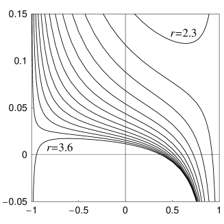
$I_{2}$: $\theta=\pi/2$ $I_{1}$: $\theta=\pi/4$

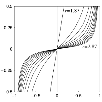
Figure 2: The invariant $I_{2}$ plotted versus relative velocity at $\theta=\pi/2$ where $I_{1}=0$ for an $a/m=1/2$ Kerr spacetime at selected radii (the situation at $\theta=\pi/4$ is not much different qualitatively) and the invariant $I_{1}$ at $\theta=\pi/4$.

6 The general solution of the transport equation along future-pointing timelike circular orbits

As shown in section 2, the solution of the parallel transport equation is (6), where $A$ is given by (36) and $\lambda=\tau$ is the proper time parametrization of the orbit when $U$ is timelike. $A$ is a tensor field only defined along the orbit and the components of $A$ can be referred to any observer-adapted frame once the observer family itself is chosen all along the orbit. Splitting $A$ into its electric part associated with a boost in an observer-adapted frame and a magnetic part associated with a rotation

$$A^{\flat}=u^{\flat}\wedge\mathcal{E}(u)+{}^{\ast_{(\hbox{$\scriptstyle u$})}}\kern-1.0pt\mathcal{B}(u)=A_{\rm B}(u)^{\flat}+A_{\rm R}(u)^{\flat}\ ,$$ (47)

can be done with respect to any stationary unit timelike future-pointing vector field $u$ representing the 4-velocity of a stationary observer family defined along the orbit, but the separation is observer-dependent.

In the general Synge nonsingular case, $A$ generates a simultaneous boost and spatial rotation acting in orthogonal 2-planes, but the frame is not adapted to these 2-planes so the boost and rotation are mixed together in their effects on the frame vectors. The two parts $A_{\rm B}(u)$ and $A_{\rm R}(u)$ do not in general commute, so $e^{A\,\tau}\neq e^{A_{\rm B}(u)\,\tau}\,e^{A_{\rm R}(u)\,\tau}$. However, one can always find one observer for which these two parts do commute, which in turn corresponds to parallel electric and magnetic fields $\mathcal{E}(u)$ and $\mathcal{B}(u)$. This has been explained in detail in [?] (exercise 20.6, p. 480) for a nonnull electromagnetic field where a new observer with relative velocity along the direction of the Poynting vector can be chosen to align the electric and magnetic fields. We use that same procedure here.

For simplicity assume $U$ is a future-pointing timelike unit vector. Start with $A^{\flat}=U^{\flat}\wedge\mathcal{E}(U)+{}^{\ast_{(\hbox{$\scriptstyle U$})}}\kern-1.0pt\mathcal{B}(U)$ as seen by $U$ itself. Pick a new circularly rotating observer with 4-velocity $\mathcal{X}(U)$ traveling in in the direction of $\mathcal{E}(U)\times_{U}\mathcal{B}(U)$ with signed relative velocity $\tanh\tilde{\alpha}$ along the $\phi$ direction within the local rest space of $U$ chosen so that

$$|\tanh\,2\,\tilde{\alpha}|=\frac{2\,||\mathcal{E}(U)\times_{n}\mathcal{B}(U)||}{\mathcal{E}(U)^{2}+\mathcal{B}(U)^{2}}\ .$$ (48)

As long as the right hand side does not equal 1 (the Synge singular case for $A$), this has a real solution. With a convenient choice of sign, direct evaluation using Eq. (5) gives

$$\tanh\,2\,\tilde{\alpha}=\frac{2\,\kappa\,\tau_{1}}{\kappa^{2}+||\omega_{\rm(FS)}||^{2}}\equiv T\ .$$ (49)

while identities then lead to

$$\tanh\,\tilde{\alpha}=\frac{1-\sqrt{1-T^{2}}}{T}\equiv t\ ,\ \sinh\,\tilde{\alpha}=\frac{t}{\sqrt{1-t^{2}}}\ ,\ \cosh\,\tilde{\alpha}=\frac{1}{\sqrt{1-t^{2}}}\ .$$ (50)

Note that the sign of $\tilde{\alpha}$ is the same as the sign of $\tau_{1}$ as long as $\kappa\geq 0$ as assumed here, while $\tilde{\alpha}$ itself reduces to 0 in the limit $\tau_{1}\to 0$ or $\kappa\to 0$ and the Frenet-Serret frame is itself adapted to the parallel transport boost and rotation. The first case of vanishing first torsion corresponds to the extremely accelerated orbits; when in addition the second torsion goes to zero as it does identically in the equatorial plane of the Kerr spacetime, this becomes a pure boost. The second case of vanishing curvature corresponds to the geodesics in the equatorial plane, which instead leads to a pure rotation in the local rest space of the geodesic. When $\tilde{\alpha}\neq 0$, its sign indicates whether one must slow down ($-$) or speed up ($+$) in the positive $\phi$-direction relative to $U$ to achieve the canonical form for the connection matrix $A^{\alpha}{}_{\beta}$.

Fig. 3 illustrates the behavior of the relative velocity $\tanh\tilde{\alpha}$. Far enough from the horizon where there are two geodesics in the equatorial plane, $\tilde{\alpha}$ is zero at the two geodesics and at the extremely accelerated orbit in between them, but as one moves in, first the extremely accelerated orbit and the counterrotating geodesic go null together, leaving one zero, and then finally the corotating geodesic goes null (not yet reached in this sequence). Similarly the values $\pm 1$ occur when the Synge singular orbits are reached at the endpoints of the boost zone, which grows outwards from $\nu=0$ as one moves towards the horizon, exiting first at $\nu=-1$ from the timelike interval. Off the equatorial plane, there is only one zero at the extremely accelerated orbit. For velocities faster than this, one must slow down, and for velocities less than this, speed up, to boost $U$ by this relative velocity.

$\theta=\pi/2$ $\theta=\pi/4$

Figure 3: The boost velocity ${\rm tanh}\,\tilde{\alpha}$ from $U$ to the parallel transport adapted frame plotted versus $\nu$, shown for $r=2,\,2.5,\,3,\,3.4,\,4$ (from solid to increasingly longer dashed lines) in the $a/m=1/2$ Kerr spacetime.

Boosting the Frenet-Serret frame vectors $\{U,\,e_{2}\}$ to $\{E_{0},\,E_{2}\}$ by the relative observer boost from $U$ to $\mathcal{X}(U)$ and defining the second pair of frame vectors $E_{1}$ and $E_{3}$ as proportional to their respective covariant derivatives gives the form

$$E_{0} = \mathcal{X}(U)=\cosh\tilde{\alpha}\,U+\sinh\tilde{\alpha}\,e_{2}\ ,$$

$$E_{2} = \bar{\mathcal{X}}(U)=\sinh\tilde{\alpha}\,U+\cosh\tilde{\alpha}\,e_{2}\ ,$$

$$E_{1} = \sigma_{\rm B}^{-1}\,[(\kappa\,\cosh\tilde{\alpha}-\tau_{1}\,\sinh\tilde{\alpha})\,e_{1}+\tau_{2}\,\sinh\tilde{\alpha}\,e_{3}]\ ,$$

$$E_{3} = \sigma_{\rm R}^{-1}\,[(\kappa\,\sinh\tilde{\alpha}-\tau_{1}\,\cosh\tilde{\alpha})\,e_{1}+\tau_{2}\,\cosh\tilde{\alpha}\,e_{3}]\ ,$$ (51)

(reducing to the identity transformation when $\tilde{\alpha}=0$) which leads to

$$A^{\flat}=-\sigma_{\rm B}\,E_{0}^{\flat}\wedge E_{1}^{\flat}+\sigma_{\rm R}\,E_{2}^{\flat}\wedge E_{3}^{\flat}\ .$$ (52)

Requiring orthogonality of $E_{1}$ and $E_{3}$ leads to the condition (49), while the invariants (recall the relations (5))

$$I_{1}=-\sigma_{\rm B}\,\sigma_{\rm R}=-\kappa\,\tau_{2}\ ,\ I_{2}=\sigma_{\rm B}^{2}-\sigma_{\rm R}^{2}=\kappa^{2}-(\tau_{1}^{2}+\tau_{2}^{2})$$ (53)

may then be used to determine the nonnegative boost parameter $\sigma_{\rm B}\geq 0$ and the rotation parameter $\sigma_{\rm R}$ in terms of the curvature and torsions

$$\sigma_{\rm B}{}^{2}=[(I_{2}{}^{2}+I_{1}{}^{2})^{1/2}+I_{2}]/2\ ,\ \sigma_{\rm R}{}^{2}=[(I_{2}{}^{2}+I_{1}{}^{2})^{1/2}-I_{2}]/2\ ,$$ (54)

equivalent to normalizing $E_{1}$ and $E_{2}$. Note that $E_{2}=\bar{\mathcal{X}}(U)$ is just the unit vector in the direction of increasing $\phi$ in the local rest space of $\mathcal{X}(U)$ and the sign of $\sigma_{R}$ must agree with the sign of $\tau_{2}$.

In the Synge semi-singular case $I_{1}=-\kappa\,\tau_{2}=0$ but $I_{2}\neq 0$, then parallel transport reduces to a pure boost ($I_{2}>0\rightarrow\sigma_{R}=0,\,\sigma_{B}=|I_{2}|^{1/2}$) under which $\bar{\mathcal{X}}(U)$ is invariant or a pure rotation ($I_{2}<0\rightarrow\sigma_{B}=0,\,\sigma_{R}=|I_{2}|^{1/2}$) under which $\mathcal{X}(U)$ is invariant. This is true in the equatorial plane of the Kerr spacetime where $\tau_{2}=0$ identically and this invariant unit vector $\bar{\mathcal{X}}(U)$ or $\mathcal{X}(U)$ respectively defines the equatorial plane map $U\to\mathcal{Z}(U)$ which picks out the direction of the covariant constant vector in the velocity plane along the orbit .${}^{\hbox{\immediate{?}}}$ For geodesics in the equatorial plane, this is a pure rotation in the local rest space of $U$ as remarked above. Figs. 4 and 5 show the typical behavior of $\sigma_{B}$ and $\sigma_{R}$.

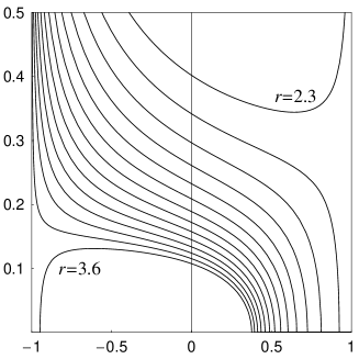
$\theta=\pi/2$ $\theta=\pi/4$

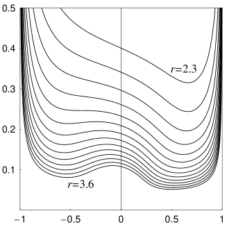
Figure 4: $\sigma_{B}$ versus $\nu$ for the $a/m=1/2$ Kerr spacetime.

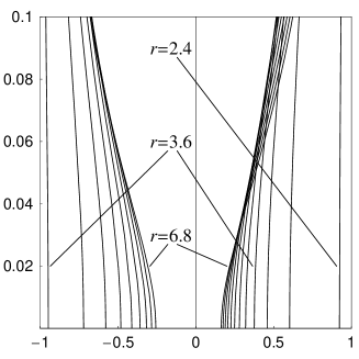
$\theta=\pi/2$        $\theta=\pi/4$

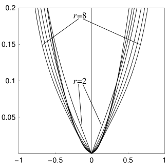
Figure 5: $\sigma_{R}$ versus $\nu$ for the $a/m=1/2$ Kerr spacetime.

To express the boosted frame in terms of the original symmetry adapted ZAMO frame, one can follow the same approach, starting with a boost

$$E_{0}=\mathcal{X}(U)=\cosh\hat{\alpha}\,n+\sinh\hat{\alpha}\,e_{\hat{\phi}}\ ,\ E_{2}=\bar{\mathcal{X}}(U)=\sinh\hat{\alpha}\,n+\cosh\hat{\alpha}\,e_{\hat{\phi}}$$ (55)

and using its inverse to re-express

$$A^{\flat}=n^{\flat}\wedge\mathcal{E}(n)+\omega^{\hat{\phi}}\wedge\mathcal{K}\ ,\ \mathcal{K}=\gamma\,\nu\,k_{\rm(fw)}$$ (56)

in the form

$$A^{\flat}=\mathcal{X}(U)^{\flat}\wedge\mathcal{E}(\mathcal{X}(U))+\bar{\mathcal{X}}(U)^{\flat}\wedge\mathcal{K}(\mathcal{X}(U))\ ,$$ (57)

where

$$\mathcal{E}(\mathcal{X}(U))=\cosh\hat{\alpha}\,\mathcal{E}(n)-\sinh\hat{\alpha}\,\mathcal{K}\ ,\ \mathcal{K}(\mathcal{X}(U))=-\sinh\hat{\alpha}\,\mathcal{E}(n)+\cosh\hat{\alpha}\,\mathcal{K}\ .$$ (58)

Then the orthogonality condition (alignment of electric and magnetic vectors)

$$0=\mathcal{E}(\mathcal{X}(U))\cdot\mathcal{K}(\mathcal{X}(U))=\bar{\mathcal{X}}(U)\cdot[\mathcal{E}(\mathcal{X}(U))\times_{\mathcal{X}(U)}\mathcal{B}(\mathcal{X}(U))]$$ (59)

yields the corresponding rapidity condition

$$\tanh 2\hat{\alpha}=\frac{\mathcal{E}(n)\cdot\mathcal{K}}{||\mathcal{E}(n)||^{2}+||\mathcal{K}||^{2}}=\frac{e_{\hat{\phi}}\cdot[\mathcal{E}(n)\times_{n}\mathcal{B}(n)]}{||\mathcal{E}(n)||^{2}+||\mathcal{B}(n)||^{2}}\ .$$ (60)

from which one can determine the ZAMO relative velocity $\nu_{\mathcal{X}}=\tanh\hat{\alpha}=[1-(1-\tanh^{2}2\hat{\alpha})^{1/2}]/\tanh 2\hat{\alpha}$ of $\mathcal{X}(U)$ in terms of $\vec{a}(n)$, $\vec{k}_{\rm(lie)}$, and $\vec{\theta}_{\hat{\phi}}$ using (4).

Now that the boost velocity is determined with respect to either the ZAMOs or $U$ itself, consider the component matrix $(A^{\alpha}{}_{\beta})$ in the new boosted frame $E_{\alpha}$, which has the canonical block-diagonal form

$$(A^{\alpha}{}_{\beta})=(A_{\rm B}{}^{\alpha}{}_{\beta})+(A_{\rm R}{}^{\alpha}{}_{\beta})=\left(\begin{array}[]{cc}\left[\begin{array}[]{cc}0&\sigma_{\rm B}\\[2.84526pt] \sigma_{\rm B}&0\end{array}\right]&\mbox{\Large 0}_{2}\vspace{3mm}\cr\mbox{\Large 0}_{2}&\mbox{\Large 0}_{2}\end{array}\right)+\left(\begin{array}[]{cc}\mbox{\Large 0}_{2}&\mbox{\Large 0}_{2}\vspace{3mm}\cr\mbox{\Large 0}_{2}&\hskip 8.53581pt\left[\begin{array}[]{cc}0&\sigma_{\rm R}\\[2.84526pt] -\sigma_{\rm R}&0\end{array}\right]\end{array}\right)$$ (61)

where $A_{\rm B}$ has eigenvalues $\lambda=0,\,0,\,\pm\sigma_{\rm B}$ and $A_{\rm R}$ has eigenvalues $\lambda=0,\,0,\,\pm i\,\sigma_{\rm R}$. This translates the action of parallel transport along the orbit for a generic vector $X$ into two commuting actions of a family of boosts and rotations when expressed in this frame

$$\dot{X}(\tau)=A\,X(\tau)\ ,\quad\rightarrow\quad X(\tau)=e^{A_{\rm B}\,\tau}\,e^{A_{\rm R}\,\tau}\,X(0)\ ,$$ (62)

so that the frame components of a parallel transported vector $X(\tau)$ in this new frame are only coupled within two mutually orthogonal subspaces

$$\pmatrix{X^{0}(\tau)\cr X^{1}(\tau)}=\pmatrix{\cosh\sigma_{\rm B}\,\tau&\sinh\sigma_{\rm B}\,\tau\cr\sinh\sigma_{\rm B}\,\tau&\cosh\sigma_{\rm B}\,\tau}\,\pmatrix{X^{0}(0)\cr X^{1}(0)}$$ (63)

$$\pmatrix{X^{2}(\tau)\cr X^{3}(\tau)}=\pmatrix{\cos\sigma_{\rm R}\,\tau&\sin\sigma_{\rm R}\,\tau\cr-\sin\sigma_{\rm R}\,\tau&\cos\sigma_{\rm R}\,\tau}\,\pmatrix{X^{2}(0)\cr X^{3}(0)}$$ (64)

and evolution of the initial data in the general case is governed respectively by a boost or a rotation in these subspaces. In the general nonsingular case, both must be present.

When $A$ is singular in the Synge sense, corresponding to vanishing values of the quantities $\sigma_{\rm B}$ and $\sigma_{\rm R}$ defined by Eqs. (54) the above derivation and the representation (52) do not hold and must be redone. Circular orbits for which $A$ is singular but nonzero cannot be geodesics but must have nonzero $\kappa=\pm\tau_{1}$ and $\tau_{2}=0$. Then the mixed component matrix of $A$ with respect to $\{u,e_{1},e_{2},e_{3}\}$ is

$$A^{\flat}=\kappa\,e_{1}\wedge[U\pm e_{2}],\qquad(A^{\alpha}{}_{\beta})=\pmatrix{0&\kappa&0&0\cr\kappa&0&\pm\kappa&0\cr 0&\pm\kappa&0&0\cr 0&0&0&0\cr}\ ,$$ (65)

which generates a null rotation

$$e^{A\tau}=1+A\,\tau+\frac{1}{2}\,A^{2}\,\tau^{2}\$$ (66)

in the plane orthogonal to $e_{3}$.

In the Kerr spacetime, this Synge singular case only occurs in the equatorial plane as the transition between the parallel transport boost and rotation velocity zones for each circular orbit .${}^{\hbox{\immediate{?}}}$ That $A^{\flat}$ is a decomposable 2-form for the Synge singular case is true for the entire Synge semi-singular case which characterizes the Kerr equatorial plane where the vanishing of $\tau_{2}$ makes $\sigma_{B}\,E_{1}$ and $\sigma_{R}\,E_{3}$ both proportional to $e_{1}$ (so only one term survives in Eq. (52), proportional to $e_{1}\wedge E_{0}$ or $e_{1}\wedge E_{2}$), which then factors out of $A^{\sharp}$ as one also sees directly from setting $\tau_{2}=0$ in Eq. (5)

$$A^{\sharp}=-\kappa\,U\wedge e_{1}+\tau_{1}\,e_{1}\wedge e_{2}=e_{1}\wedge(\kappa\,U+\tau_{1}\,e_{2})\ .$$ (67)

When the vector in parentheses is nonnull, it is proportional to $E_{0}=\mathcal{X}(U)$ if timelike ($I_{1}>0$) corresponding to a parallel transport boost or $E_{2}=\bar{\mathcal{X}}(U)$ if spacelike ($I_{2}<0$) corresponding to a parallel transport rotation, and taking the parametrization relationship (21) into account, while choosing instead $e_{1}=e_{\hat{r}}$ (allowing $\kappa$ to change sign), one can translate this back to the map $\mathcal{Z}$ determining the invariant parallel transport direction using (A.7) of [?].

7 Boost and rotation domination zones

The Synge class of the matrix $A$ associated with the invariants $I_{1}$ and $I_{2}$ is a function of the two nonignorable coordinates $r$ and $\theta$. Either $I_{2}\neq 0$ (nonsingular case) or $I_{1}=0$ but $I_{2}\neq 0$ (semi-singular case) or $I_{1}=0=I_{2}$ (singular case), each case corresponding to a different class of Lorentz transformations governing parallel transport.

The sign of $I_{2}$ indicates the relative magnitudes of the boost and rotation rates along a circular orbit in the nonsingular case (boost-dominated if $I_{2}>0$, rotation-dominated if $I_{2}<0$) and whether a pure boost ($I_{2}>0$) or pure rotation ($I_{2}<0$) occurs in the semi-singular case. Such boost-dominated and rotation-dominated zones occur in each family of circular orbits at a given radius and angular location as a function of the relative velocity, but as one approaches the vicinity of the horizon in a Kerr spacetime, for timelike circular orbits the rotation-dominated zones disappear as the attraction to the black hole (acceleration) overcomes any relative centripetal acceleration effects (Frenet-Serret angular velocity) due to the limits on the relative velocity $|\nu|<1$.

For a given radial and angular position of a circular orbit, the condition $I_{2}=0$ determines two relative velocities which delimit an interval $\nu_{(PT-)}<0<\nu_{(PT+)}$ around the ZAMO angular velocity $\nu=0$ within which parallel transport boost-dominance occurs ($I_{2}>0$)

$$|\kappa|>||\omega_{\rm FS}||\leftrightarrow||\mathcal{E}(n)||>||\mathcal{B}(n)||\leftrightarrow||F^{(G)}_{\rm(fw)}||>\gamma\,\nu||k_{\rm(fw)}||\ .$$ (68)

and the Fermi-Walker relative gravitational force on the circular orbit exceeds the Fermi-Walker relative angular velocity. Using (4) one can express this inequality as a quadratic inequality in $\nu$

$$I_{2} = (||\theta_{\hat{\phi}}||^{2}-||k_{\rm(lie)}||^{2})\,\nu^{2}-2\,\theta_{\hat{\phi}}\cdot(g+k_{\rm(lie)})\,\nu+||g||^{2}-||\theta_{\hat{\phi}}||^{2}$$ (69)

$$= -\mathcal{A}\,\nu^{2}-2\,\mathcal{B}\,\nu+\mathcal{C}>0$$

whose corresponding equality has the solutions $\nu_{\rm(PT-)}\leq\nu_{\rm(PT+)}$ given by the minimum and maximum values of the usual quadratic formula for the roots

$$\nu_{\rm(PT\pm)}=\frac{-\mathcal{B}\pm[\mathcal{B}^{2}+\mathcal{A}\,\mathcal{C})]^{1/2}}{\mathcal{A}}\ .$$ (70)

This leads to the static limit

$$\theta_{\hat{\phi}}\to 0:\quad\nu_{\rm(PT\pm)}\to\frac{||\vec{g}||}{||k_{\rm(lie)}||}\left(\pm 1-\frac{\theta_{\hat{\phi}}\cdot(g+k_{\rm(lie)})}{||g||\,||k_{\rm(lie)}||}\right)\ ,$$ (71)

with $\mathcal{B}=\theta_{\hat{\phi}}\cdot(g+k_{\rm(lie)})>0$ for a corotating ($a>0$) Kerr spacetime ${}^{\hbox{\immediate{?}}}$ and $\mathcal{A}=||k_{\rm(lie)}||^{2}-||\theta_{\hat{\phi}}||^{2}>0$ holds everywhere except very close to the horizon.

When the relative velocity moves out of the interval $[\nu_{\rm(PT-)},\,\nu_{\rm(PT+)}]$, the circular orbit has sufficient speed for the relative Fermi-Walker angular velocity to exceed the Fermi-Walker spatial gravitational force. Inside this interval the Fermi-Walker spatial gravitational force dominates the relative angular velocity. At these endpoint values, the circular orbit parallel transports one of the two circular null tangent vectors, as shown by Eq. (45); in the equatorial plane, $A$ is then singular generating a null rotation as described in [?].

The condition $\nu_{\rm(PT\pm)}=\pm 1$, after clearing fractions, isolating the radical and squaring both sides of the resulting equation, becomes $\mathcal{A}\,(\mathcal{A}\pm 2\,\mathcal{B}-\mathcal{C})=0$. Setting the second factor to zero yields

$$(a(n)-k_{\rm(lie)})\cdot(a(n)+k_{\rm(lie)}\pm 2\,\theta_{\hat{\phi}})=0\leftrightarrow\vec{a}_{0}\cdot\vec{a}_{\pm}=0$$ (72)

which shows that these limiting null orbits occur when the position vector $\vec{a}_{0}=-\vec{g}_{+}$ of the center of the acceleration hyperbola is perpendicular to one of the two asymptote directions $\vec{a}_{\pm}$ corresponding to null orbits, or if $\vec{a}_{0}$ vanishes, or if one of those null circular orbit acceleration vectors vanishes. The latter corresponds to corotating and counterrotating null circular geodesics, which occur in the equatorial plane of the Kerr spacetime.

The limits $\nu_{\rm(PT\pm)}\to\pm\infty$ correspond to $\bar{\nu}_{\rm(PT\pm)}=1/\nu_{\rm(PT\pm)}\to 0^{\pm}$ which describe the spacelike closed $\phi$-coordinate circles. These occur where the leading coefficient $-\mathcal{A}=||\theta_{\hat{\phi}}||^{2}-||k_{\rm(lie)}||^{2}$ goes to zero in the above quadratic relationship (69) for the root where no cancellation occurs in the numerator in this limit. But for null relative velocities $\nu=\pm 1$, one has $k_{\rm(fw)}=k_{\rm(lie)}+(\pm 1)\,\theta_{\hat{\phi}}$, so this will occur at locations $(r,\,\theta)$ where the Fermi-Walker curvature for one of the two null orbits vanishes, corresponding to a “Fermi-Walker relatively straight” curve, where the Fermi-Walker relative centripetal acceleration goes to zero.

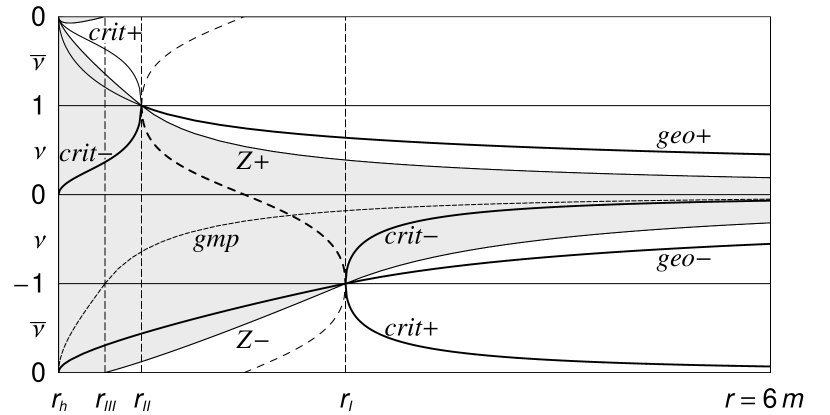
Figure 6: The boost- (grey shading) and rotation-dominated (white) relative velocity zones for the equatorial plane in the $a/m=1/2$ Kerr spacetime for $-\infty<\nu<\infty$ using the reciprocal velocity $\bar{\nu}=1/\nu$ to plot the spacelike relative velocities $|\nu|>1$, with the top and bottom borders identified to describe the same closed $\phi$ circles being traced out in opposite directions. The velocity curves labeled by $Z_{\pm}=\nu_{\rm(PT\pm)}$ separate these two zones. Vertical lines indicate the radii at which the counterrotating ($r_{I}$) and corotating ($r_{II}$) geodesics go null, the radius $r_{III}$ where the geodesic meeting point orbits go null and the horizon $r_{h}$ where the null meeting point orbits (ZAMO world lines outside the horizon, see [?]) go null. These correspond respectively to the radii where $\nu_{\rm(PT-)}=-1$ ($I$), $\nu_{\rm(PT+)}=1$ ($II$), $\nu_{\rm(PT-)}\to-\infty$ $(III$) and $\nu_{\rm(PT+)}\to\infty$. Also shown are the relative velocity profiles of the geodesics (geo$\pm$), geodesic meeting point curves (gmp), and the critical points of the circular orbit acceleration where $\tau_{1}=0$ (crit$\pm$). The subluminal critical point curve (crit$-$) corresponds to the extremely accelerated observers. The dashed curve between the radii $r_{I}$ and $r_{II}$ shows instead the critical points of $\tau_{1}=|\omega_{\rm(FS)}|$.

For a corotating Kerr spacetime, as one moves closer to the black hole in the equatorial plane ,${}^{\hbox{\immediate{?},\penalty 1000\hskip 0.91003pt plus 0.70004pt minus 0.70004pt{\bf{?}}}}$ the interval $[\nu_{\rm(PT-)},\,\nu_{\rm(PT+)}]$ expands until $\nu_{\rm(PT-)}=-1$ at the counterrotating null circular geodesic so that counterrotating rotation-dominated timelike orbits no longer exist and then continues until finally $\nu_{\rm(PT+)}=1$ at the corotating null circular geodesic so that not even corotating rotation-dominated timelike orbits exist beyond that .${}^{\hbox{\immediate{?}}}$ In the equatorial plane these occur exactly at the counterrotating ($r_{I}$) and corotating ($r_{II}$) null geodesic orbits, while $\nu_{\rm(PT-)}\to-\infty$ at the geodesic meeting point observer horizon ($r_{III}$) and $\nu_{\rm(PT+)}\to\infty$ at the black hole horizon (ZAMO horizon: $r_{h}$), corresponding to transport around closed $\phi$ coordinate loops .${}^{\hbox{\immediate{?}}}$ Fig. 6 shows the boost-dominated zone (or just boost zone since there is no simultaneous rotation) shaded in grey, with the remaining rotation-dominated zone (or just rotation zone) in white. This explains the domains of $\sigma_{B}$ (inside the boost zone) and $\sigma_{R}$ (outside the boost zone) respectively in Figs. 4$a)$ and 5$a)$, while off the equatorial plane both quantities are defined for all velocities except $|\nu|\to 1$ where they both go infinite due to a gamma factor in their definition.

Figure 7: A polar plot in the $r$-$\theta$ plane treated as though they were polar coordinates in a flat 2-space with horizontal axis $\rho=(r/m)\sin\theta$ and vertical axis $z=(r/m)\cos\theta$, for an $a/m=1/2$ Kerr spacetime, showing the event horizon (h, thick curve), where $\nu_{\rm(PT+)}\to\infty$, the ergosphere boundary (e, dashed curve), the curve $I$ where $\nu_{\rm(PT-)}=-1$ and the curve $II$ where $\nu_{\rm(PT+)}=1$ , and finally the curve $III$ intersecting the horizon at about $19^{o}$ above the equatorial plane, along which $\nu_{\rm(PT-)}\to-\infty$ from the outside, but $\infty$ from the inside (see Fig. 6).

Fig. 7 extends these boundary regions off the equatorial plane to show the horizon, ergosphere boundary and the curves in an $r$-$\theta$ section of the exterior Kerr spacetime where $\nu_{\rm(PT\pm)}$ take the values $\pm 1$ and have the limits $\pm\infty$. The first two conditions define two closed surfaces of revolution surrounding the horizon and ergosphere boundary, the II surface (corotating) inside the I surface (counterrotating), which both meet the horizon and ergosphere at the symmetry axis $\theta=0$ but extend farther out from them and each other as one approaches the equatorial plane, which they intersect in circles at the respective radii where the corotating null geodesics and counterrotating null circular geodesics exist. The limit $\nu_{\rm(PT-)}\to-\infty$ (approaching from the side away from the origin, but $\infty$ when approaching from inside) occurs along the smaller curve III in Fig. 7 near the equatorial plane up to about $\theta=71^{o}$ where it intersects the horizon, where in turn the limit $\nu_{\rm(PT+)}\to\infty$ occurs.

In the static Schwarzschild limit, the surfaces corresponding to the curves $I$ and $II$ in Fig. 7 come together at the radius $r=3\,m$ in the equatorial plane, while the horizon, ergosphere boundary and the infinite limit surfaces collapse to the sphere $r=2\,m$ (see Fig. 2 of ?). Inside the single surface $I=II$, no timelike timelike circular orbit exists with rotation-domination. In the general Kerr spacetime, inside of the outermost surface $I$, no timelike counterrotating circular orbit exists with parallel transport rotation-domination, while inside the next surface $II$, no timelike corotating or counterrotating timelike circular orbit exists with rotation-domination. Inside the next surface $III$, no counterrotating circular orbit of any causality type exists with rotation-domination, while at the horizon all circular orbits of any kind are boost-dominated as the rotation-domination velocity zone shrinks to the null set at the closed $\phi$-coordinate circle being traversed in the corotating direction of increasing $\phi$, exactly as in the equatorial plane in Fig. 6.

$a)$ $\theta=1.5$

$b)$ $\theta=\pi/3$

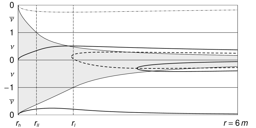
Figure 8: The figure corresponding to Fig. 6 off the equatorial plane ($\theta=\pi/2\approx 1.57$) nearby at $\theta=1.5$ and farther away at $\theta=\pi/3$. Vanishing $\tau_{1}$ occurs at the solid curves (not bounding the grey region), while the dashed curve indicates the zero of its $\nu$-derivative. In $a)$ one sees that departing from the equatorial plane, the geo$-$ and counterotating crit$-$ curves to the right of $r_{I}$ in the equatorial plane Fig. 6 deform and join together to produce the subluminal counterrotating vanishing $\tau_{1}$ curve, while the geo$+$ curve and the corotating crit$-$ curve similarly produce the corotating such subluminal curve; the counterrotating superluminal crit$+$ curve joins together with the superluminal geo$-$ curve to produce the the superluminal counterrotating vanishing $\tau_{1}$ curve. The boost zone shrinks with decreasing angle. The dashed-dotted uppermost curve in the white rotation-dominated zone corresponds to vanishing $\tau_{2}$ at positive superluminal speeds (converging with the boost-dominated zone boundary curves at the horizon at $\bar{\nu}=0$), while the subluminal such curve occurs at very small negative relative velocities not distinguishable from the $\nu$-axis at this scale.

One can imagine how this latter figure changes as one decreases $\theta$ from $\pi/2$ in Fig. 6. Fig. 8$a)$ shows how the equatorial plane velocity curves deform and join to produce the vanishing $\tau_{1}$ velocity curves as the boost zone squeezes down towards $\nu=0$ and its marking radii move in towards the horizon as $\theta$ decreases. This continues in $b)$, where the radius $r_{III}$ has already disappeared inside the horizon, and is the result of the fact that at a fixed radius, decreasing $\theta$ also decreases the flat space circular radius $\rho=r\,\sin\theta$, which increases the centripetal acceleration roughly by $1/\rho$ compared to the central attraction which does not dramatically change with angle. This in turn increases the parallel transport rotation-dominated zone compared to the boost-dominated zone. The fact that the velocity profile corresponding to $\tau_{2}=0$ (where $I_{1}=0$), which determines the extremum of the acceleration polar angle $\chi$, is an extremely small negative function at these scales (explaining why all the $I_{1}$ curves appear to pass through the origin in Fig. 2) shows that this point on the acceleration hyperbola is just slightly to the counterrotating side of the ZAMO point.

In the case of the equatorial plane of the Kerr spacetime discussed extensively in [?], the acceleration is purely radial corresponding to $\chi=0,\,\pi$ which makes its $\chi$-derivative and hence $\tau_{2}$ identically zero. Thus $A$ is always semi-singular and becomes singular at the boundary between boost and rotation dominance where $|\kappa|=|\tau_{1}|$. This occurs for

$$\nu_{(PT\pm)}=\frac{\nu_{\rm(gmp)}\mp\nu_{+}\,\nu_{-}}{1\mp\nu_{\rm(gmp)}}\ ,\quad\nu_{\rm(gmp)}=(\nu_{+}+\nu_{-})/2\ ,$$ (73)

where $\nu_{\rm(gmp)}$ is the velocity of the geodesic meeting point trajectories ,${}^{\hbox{\immediate{?}}}$ or explicitly

$$\nu_{(PT\pm)}=\frac{m\left[a\,(r-m)\,(a^{2}+3\,r^{2})\pm(r^{3}+a^{2}\,r+2\,a^{2}\,m)\,\sqrt{\Delta}\right]}{(-r^{4}+2\,m\,r^{3}+2\,a^{2}\,m\,r+a^{2}\,m^{2})\,\sqrt{\Delta}}\ .$$ (74)

Notice that from the formula (73), the values the values $\nu_{(PT\pm)}=\pm 1$ occur when respectively $\nu_{\pm}=\pm 1$, so that the respective endpoints of the boost-dominated zone go null at the same radii as the counter-rotating ($r_{I}$) and then the corotating circular geodesics ($r_{II}$) go null as one approaches the horizon. Similarly, for example, as $\nu_{\rm(gmp)}\to-1^{+}$, then $\nu_{\rm(PT-)}\to-\infty$, which occurs at $r_{III}$ in Fig. 6. This feature of the geodesic meeting point horizon in the equatorial plane was uncovered in studies of circular holonomy started by Rothman et al .${}^{\hbox{\immediate{?},\penalty 1000\hskip 0.91003pt plus 0.70004pt minus 0.70004pt{?},\penalty 1000\hskip 0.91003pt plus 0.70004pt minus 0.70004pt{?}}}$

From Eqs. (4.9) and (4.10) of [?], the conditions $\nu_{\pm}=\pm 1$ are equivalent to $\nu_{\rm(crit)\pm}=\pm 1$, so in turn the conditions $\nu_{(PT-)}=-1$ and $\nu_{(PT+)}=1$ correspond to the horizons $r_{I}$ and $r_{II}$ of the extremely accelerated orbits in the equatorial plane, which are critical points of the acceleration as a function of the relative velocity, labeled as crit$\pm$ in Fig. 6. This explains the triple crossing points of the geodesic velocities, extremely accelerated velocities and the boost zone endpoint velocities in that figure. The solutions of the conditions $\nu_{(PT\pm)}=\pm 1$, when fractions are cleared (numerator equals plus or minus the denominator) to produce polynomial equations in $r$ after some manipulation to eliminate the radical, have a common factor $4\,a^{2}\,m-9\,m^{2}\,r+6\,m\,r^{2}-r^{3}$, whose zeros produce the radii $r_{I}$ and $r_{II}$ of the pair of null circular geodesics. The zero of the denominator of Eq. (74) is instead $r_{III}=r_{\rm(gmp)}$, the horizon of the geodesic meeting point observers.

As $a/m$ increases from the value $1/2$ of Fig. 6 to the extreme limit $a/m=1$ in the equatorial plane, the radius $r_{II}$ shrinks down to the horizon $r_{\rm(hor)}$ crossing over $r_{III}$ as shown in Fig. 2 of ${}^{\hbox{\immediate{?}}}$ where these radii are labeled respectively by “geo₊,” “gmp” and “hor.” In fact very interesting changes occur in the interval of values $[0.89,1]$ for $a/m$ as illustrated in the polar plots of Fig. 9. As the surface $II$ shrinks down to the horizon, the surfaces $III$ and $I$ both bubble upwards and outwards, with surface $I$ developing a transversal intersection with the horizon only at the limiting value $a/m=1$ of an extreme Kerr spacetime. That surface $II$ shrinks to the horizon in this limit means that there always exists a rotation-dominated zone for sufficiently fast but subluminal corotating orbits outside the horizon. The increasing separation between the horizon and surface $III$ away from the North pole in this limit means that the corresponding small piece of grey boost-dominated region at the top left corner of Figs. 6 and 8$a)$ grows outward and downward as the lower grey zone falls downward following the rotation-dominated region as its lower border in turn moves downwards. Simultaneously the counterrotating boost-dominated region moves outward from the horizon away from the North pole. Thus the faster the spacetime rotates, the worse things are for the counterrotating orbits, which go superluminal farther and farther away from the shrinking horizon leading to boost-domination inside that radius for all subluminal motion. At the same time the corotating orbits go superluminal closer and closer to the horizon, with expanding rotating-dominated zones existing for suitably fast but subluminal motion outside that radius.

Figure 9: The figure corresponding to Fig. 7 as $a/m$ increases from 1/4 towards the extreme value 1. The surface $II$ collapses to the horizon, while the surfaces $I$ and $III$ bubble upwards and outwards (like the ergosphere boundary which they cross) to form two doughnut-like rings (when revolved about the $z$-axis) around the horizon, one inside the other. In the Schwarzschild limit $a/m\to 0$, the surfaces $I$ and $II$ collapse together to a single surface meeting the equatorial plane at $r/m=3$, while the ergosphere boundary and surface $III$ collapse together to the horizon.

8 Concluding remarks

The gravitoelectromagnetic analysis of parallel transport of the 4-velocity along generic circular orbits in stationary axisymmetric spacetimes has been extended to parallel transport of the full tangent space and connected to the corresponding Serret-Frenet description. The electromagnetic decomposition of the parallel transport matrix is essential to putting it into a canonical form for interpretation. Crucial features of parallel transport take place at the surfaces where various geometrically defined 4-velocities become null. These results enable the previous discussion of the equatorial plane of the Kerr spacetime to be extended to the whole exterior spacetime outside the horizon.

One finds new surfaces surrounding a black hole which intrinsically characterize limiting parallel transport properties along circular orbits of all causality types. Within these surfaces, one has an invariant characterization of the domination of centripetal acceleration effects by attractive forces, differing of course for corotating and counterrotating orbits. Examining the way in which the gravitoelectric, gravitomagnetic and space curvature effects enter into the parallel transport matrix and the resulting 4-acceleration gives some more insight into how centripetal acceleration and gravitational attraction compete with each other and are in turn affected by gravitomagnetic effects in the Kerr spacetime, thus complementing the results of previous work.${}^{\hbox{\immediate{?}}}$

Appendix A Geometry of the acceleration and Frenet-Serret angular velocity curves

Using the defining condition for the MIROs (vertex observers), (see the paragraph containing equation (6.3) of [?]) $e^{2\alpha_{\rm(vert)}}=\sqrt{||\vec{a}_{-}||/||\vec{a}_{+}||}$, and introducing the quantity ${\cal A}=\sqrt{||\vec{a}_{-}||||\vec{a}_{+}||}/2$, the definitions of section 4 together with the decomposition $a_{\pm}=||\vec{a}_{\pm}||\,\vec{n}_{\pm}$ into lengths and unit direction vectors lead to

$$(\vec{a}-\vec{a}_{0}) = \frac{1}{4}\left[||\vec{a}_{+}\,||e^{2\alpha}\,\vec{n}_{+}+||\vec{a}_{-}||\,e^{-2\alpha}\,\vec{n}_{-}\right]$$

$$= \frac{\cal A}{2}\,[e^{2(\alpha-\alpha_{\rm(vert)})}\,\vec{n}_{+}+e^{-2(\alpha-\alpha_{\rm(vert)})}\,\vec{n}_{-}]$$

$$= \frac{\cal A}{2}\,[\cosh 2(\alpha-\alpha_{\rm(vert)})\,(\vec{n}_{+}+\vec{n}_{-})+\sinh 2(\alpha-\alpha_{\rm(vert)})\,(\vec{n}_{+}-\vec{n}_{-})]\ .$$

Here $\alpha=\mbox{arctanh}\,\nu$ is the rapidity parametrization of the acceleration curve.

The photon acceleration direction vectors, which determine the common asymptotes of the acceleration and Frenet-Serret angular velocity hyperbolas, are independent of the reference observer family used to decompose the acceleration. It is natural to introduce the unit direction vectors of their sum and difference which determine the common orthogonal axes of the acceleration hyperbola.

The opening angle $\beta\in[0,\,\pi]$ of the acceleration hyperbola (making $\pi-\beta$ the opening angle of the Frenet-Serret angular velocity hyperbola) satisfies $\vec{n}_{+}\cdot\vec{n}_{-}=\cos\beta$, in terms of which one finds

$$||\vec{n}_{+}+\vec{n}_{-}||/2=\cos\frac{\beta}{2}\ ,\quad||\vec{n}_{+}-\vec{n}_{-}||/2=\sin\frac{\beta}{2}\ ,$$

leading to the orthogonal unit vectors

$$\vec{\mbox{\i}}=\frac{\vec{n}_{+}+\vec{n}_{-}}{2\,\cos\frac{\beta}{2}}\ ,\qquad\vec{\mbox{\j}}=\frac{\vec{n}_{+}-\vec{n}_{-}}{2\,\sin\frac{\beta}{2}}$$ (76)

which give the directions of the principal axes of both hyperbolas. The quantities ${\cal A}\,\cos\frac{\beta}{2}$ and ${\cal A}\,\sin\frac{\beta}{2}$ are the semi-axis parameter lengths of the acceleration and the Frenet-Serret angular velocity hyperbolas. By introducing the sign $\epsilon$ which makes the following cross-product relation valid

$$\epsilon\,\vec{\mbox{\i}}\times_{n}\vec{\mbox{\j}}=e_{\hat{r}}\times_{n}e_{\hat{\theta}}=e_{\hat{\phi}}\ ,$$ (77)

and whose value in the Kerr spacetime is $\epsilon={\rm sgn}(\pi/2-\theta)$, one can finally write the equations for the acceleration and angular velocity hyperbolas in terms of their geometric properties

$$\vec{a}-\vec{a}_{0}={\cal A}\,[\cosh 2(\alpha-\alpha_{\rm(vert)})\,\cos\frac{\beta}{2}\;\vec{\mbox{\i}}+\sinh 2(\alpha-\alpha_{\rm(vert)})\,\sin\frac{\beta}{2}\;\vec{\mbox{\j}}]\ ,$$

$$\epsilon\,\vec{\omega}_{\rm(FS)}={\cal A}\,[\cosh 2(\alpha-\alpha_{\rm(vert)})\,\sin\frac{\beta}{2}\,\vec{\mbox{\i}}-\sinh 2(\alpha-\alpha_{\rm(vert)})\,\cos\frac{\beta}{2}\,\vec{\mbox{\j}}]\ .$$ (78)

It is then easy to derive the following formulas for the acceleration and angular velocity scalars

$$2(\vec{a}-\vec{a}_{0})\cdot\vec{\omega}_{\rm(FS)} = {\cal A}^{2}\sin\beta\ ,$$

$$||\vec{a}-\vec{a}_{0}||^{2} = \frac{1}{2}\,{\cal A}^{2}[\cosh 4(\alpha-\alpha_{\rm(vert)})+\cos\beta]\ ,$$

$$||\vec{\omega}_{\rm(FS)}||^{2} = \frac{1}{2}\,{\cal A}^{2}[\cosh 4(\alpha-\alpha_{\rm(vert)})-\cos\beta]\ ,$$ (79)

or equivalently

$$||\vec{a}-\vec{a}_{0}||^{2}-||\vec{\omega}_{\rm(FS)}||^{2} = {\cal A}^{2}\cos\beta\ ,$$

$$||\vec{a}-\vec{a}_{0}||^{2}+||\vec{\omega}_{\rm(FS)}||^{2} = {\cal A}^{2}\cosh 4\,(\alpha-\alpha_{\rm(vert)})\ .$$ (80)

Appendix B Frenet-Serret frame for circular orbits

The sign conventions for the Frenet-Serret scalars and the corresponding directional choices of the frame vectors for nonnull circular orbits in stationary axisymmetric spacetimes require careful consideration .${}^{\hbox{\immediate{?}}}$ Starting from the rapidity parametrized 4-velocity for a future-pointing timelike circular orbit

$$U=\cosh\alpha\,n+\sinh\alpha\,e_{\hat{\phi}}=e_{0}$$ (81)

expressed in a Boyer-Lindquist-like ZAMO orthonormal frame $\{n,\,e_{\hat{r}},\,e_{\hat{\theta}},\,e_{\hat{\phi}}\}$, one can introduce a unit vector in the direction of increasing $\phi$ in the local rest space of $U$, namely

$$e_{2}=\frac{\partial}{\partial\alpha}\,U=\sinh\alpha\,n+\cosh\alpha\,e_{\hat{\phi}}\ ,$$ (82)

thus defining two Frenet-Serret vectors in the circular orbit velocity plane so that $e_{0}\wedge e_{2}=n\wedge e_{\hat{\phi}}$. It remains to be seen that $e_{2}$ is actually a possible choice.

Next one introduces polar coordinates in the acceleration plane spanned by $\{e_{\hat{r}},\,e_{\hat{\theta}}\}$ to parametrize the acceleration vector, with a nonnegative radial coordinate

$$a(U)=\kappa\,(\cos\chi\,e_{\hat{r}}+\sin\chi\,e_{\hat{\theta}})=\kappa\,e_{1}\ ,\quad\kappa\geq 0\ ,$$ (83)

so that $e_{1}$ is the unit direction of $a(U)$ and $e_{3}$ is the orthogonal unit vector

$$e_{3}=-\frac{\partial}{\partial\chi}\,e_{1}=\sin\chi\,e_{\hat{r}}-\cos\chi\,e_{\hat{\theta}}\ ,$$ (84)

satisfying

$$e_{\hat{\phi}}\times_{n}e_{1}=-e_{3}\ ,\quad e_{\hat{\phi}}\times_{n}e_{3}=e_{1}\ ,\quad e_{3}\wedge e_{1}=e_{\hat{r}}\wedge e_{\hat{\theta}}\ ,$$ (85)

and so $e_{0}\wedge e_{1}\wedge e_{2}\wedge e_{3}=n\wedge e_{\hat{r}}\wedge e_{\hat{\theta}}\wedge e_{\hat{\phi}}$. Since $n$ and $e_{0}$ both future-pointing timelike vectors, the Frenet-Serret spatial triad is also right-handed.

To show that $e_{2}$ and $e_{3}$ can consistently be chosen as the remaining Frenet-Serret vectors, the transformation (39) of the connection matrix $A$ must be used together with the identifications (5), leading to

$$\pmatrix{-\kappa\,e_{1}\cr\tau_{2}\,e_{1}+\tau_{1}\,e_{3}\cr} = M(2\alpha)\pmatrix{g_{-}\cr H\cr}+\pmatrix{g_{+}\cr 0\cr}$$ (86)

$$= \pmatrix{\cosh 2\alpha\,g_{-}+\sinh 2\alpha\,e_{\hat{\phi}}\times_{n}H+g_{+}\cr-\sinh 2\alpha\,e_{\hat{\phi}}\times_{n}g_{-}+\cosh 2\alpha\,H\cr}\ .$$

Then since $g_{+}$ is independent of $\alpha$ and $e_{\hat{\phi}}\times_{n}(e_{\hat{\phi}}\times_{n}H)=-H$, the Frenet-Serret angular velocity can be rewritten as

$$\tau_{2}\,e_{1}+\tau_{1}\,e_{3} = \frac{1}{2}\,e_{\hat{\phi}}\times_{n}\frac{d}{d\alpha}(\kappa\,e_{1})=\frac{1}{2}\,\frac{\partial\kappa}{\partial\alpha}\,e_{\hat{\phi}}\times_{n}e_{1}+\frac{1}{2}\,\kappa\,\frac{\partial\chi}{\partial\alpha}\,e_{\hat{\phi}}\times_{n}\frac{\partial e_{1}}{\partial\chi}$$ (87)

$$= -\frac{1}{2}\,\frac{\partial\kappa}{\partial\alpha}\,e_{3}-\frac{1}{2}\,\kappa\,\frac{\partial\chi}{\partial\alpha}\,e_{1}\ .$$

Thus everything is consistent if one makes the identification

$$\tau_{1}=-\frac{1}{2}\,\frac{d\kappa}{d\alpha}\ ,\qquad\tau_{2}=-\frac{1}{2}\,\kappa\,\frac{d\chi}{d\alpha}\ .$$ (88)

The Frenet-Serret angular velocity is then given by the rapidity derivative formula

$$\omega_{\rm(FS)}=\frac{1}{2}\,e_{\hat{\phi}}\times_{n}\frac{{\rm d}a(U)}{{\rm d}\alpha}=\cosh 2\alpha\,H-\sinh 2\alpha\,e_{\hat{\phi}}\times_{n}g_{-}\ .$$ (89)

Note that interchanging the hyperbolic functions in (81) leads to the corotating spacelike case for $U$, which only interchanges $U$ and $e_{2}$, resulting in the same identifications (88) and the same first equation of (89). It remains to check all these signs for the remaining two cases of the four sign combinations for parametrizing $U$ by a hyperbolic angle $\alpha$ as in Eq. (3).

References

- [1] B.R. Iyer and C.V. Vishveshwara, Phys. Rev. D48, 5706 (1993).
- [2] R.D Greene, E.L. Schücking and C.V. Vishveshwara, J. Math. Phys. 16, 153 (1975).
- [3] C.W. Misner, K.S. Thorne and J.A. Wheeler, Gravitation, (San Francisco: Freeman), 1973.
- [4] F. de Felice, Class. Quantum Grav. 12, 1119 (1991); F. de Felice and S. Usseglio-Tomasset, Class. Quantum Grav. 8, 1871 (1991).
- [5] D. Page, Class. Quant. Grav. 15, 1669 (1998).
- [6] O. Semerák, Gen. Relativ. Grav. 30, 1203 (1998).
- [7] D. Bini, F. de Felice and R.T. Jantzen, Centripetal acceleration and centrifugal force in general relativity in Nonlinear Gravitodynamics. The Lense-Thirring effect, Ed. R. Ruffini and C. Sigismondi (Singapore: World Scientific), 2003.
- [8] D. Bini, F. de Felice and R.T. Jantzen, Class. Quantum Grav. 16, 2105 (1999).
- [9] D. Bini, R.T. Jantzen and A. Merloni, Class. Quantum Grav. 16, 1333 (1999).
- [10] J.L. Synge, Relativity: The General Theory, North Holland Amsterdam, 1960.
- [11] R.T. Jantzen, P. Carini and D. Bini, Ann. Phys. (N.Y.), 215, 1 (1992).
- [12] D. Bini, P. Carini and R.T. Jantzen, Int. J. Mod. Phys. D6, 1 (1997).
- [13] D. Bini, P. Carini and R.T. Jantzen, Int. J. Mod. Phys. D6, 143 (1997).
- [14] D. Bini, P. Carini and R.T. Jantzen, Class. Quantum Grav. 12, 2549 (1995).
- [15] D. Bini, R.T. Jantzen and B. Mashhoon, Class. Quantum Grav. 19, 17 (2002).
- [16] T. Rothman, G.F.R. Ellis and J. Murugan, Class. Quantum Grav. 18, 1217 (2001).
- [17] R. Maartens, B. Mashhoon and D.R. Matravers, Class. Quantum Grav. 19, 195 (2002).
- [18] D. Bini, R.T. Jantzen and B. Mashhoon, Class. Quantum Grav. 18, 653 (2001).
- [19] D. Bini, C. Cherubini and R.T. Jantzen, Class. Quantum Grav. 19, 5481 (2002).
- [20] J.L. Synge, Relativity: The Special Theory (2nd Edition), Chapter IV, North Holland Amsterdam, 1965.
- [21] C.G. Bollini, J.J. Giambiagi and J. Tiomno, Lett. Nuovo Cim. 31, 1 (1981).
- [22] D. Bini, F. de Felice and R.T. Jantzen, Class. Quantum Grav. 16, 2105 (1999).
- [23] D. Bini and R.T. Jantzen, Proceedings of the Ninth ICRA Network Workshop on Fermi and Astrophysics, eds. V. Gurzadyan and R. Ruffini, World Scientific, Singapore, 2003.