Post-processed time-delay interferometry for LISA

Abstract

High-precision interpolation of LISA phase measurements allows signal reconstruction and formulation of Time-Delay Interferometry (TDI) combinations to be conducted in post-processing. The reconstruction is based on phase measurements made at approximately 10 Hz, at regular intervals independent of the TDI delay times. Interpolation introduces an error less than $1\times 10^{-8}$ with continuous data segments as short as two seconds in duration. Potential simplifications in the design and operation of LISA are presented.

I Introduction

The Laser Interferometer Space Antenna (LISA) is a mission to detect gravitational waves in the frequency band from 0.1 mHz to 1 Hz. The LISA constellation consists of three spacecraft flying in a heliocentric, Earth-trailing orbit, with separations of $L\approx 5\times 10^{9}$ m. Each spacecraft contains two proof masses that are shielded from external disturbances. To detect a passing gravitational wave, the change in separation $\delta L$ of the proof masses in different spacecraft must be monitored with a precision of $\delta L/L\lesssim 10^{-20}/\sqrt{\rm{Hz}}$ using laser interferometry. This fractional length stability is far better than the fractional frequency stability of the laser source, which is expected to be $\delta\nu/\nu\gtrsim 10^{-14}/\sqrt{\rm{Hz}}$. Degradation in sensitivity due to laser frequency noise could be avoided by operating the constellation as a Michelson interferometer with equal armlengths. Unfortunately, the orbital dynamics of the constellation make it impracticable to equalize the LISA armlengths accurately enough to cancel the excess frequency noise. Time delay interferometry (TDI) Tinto is a technique to remove the otherwise overwhelming laser frequency fluctuations. TDI cancels laser frequency noise by combining phase measurements made at different times. The required timing of the measurements is set by the light travel times between the LISA spacecraft, and it must be accurate to 100 ns to meet the laser frequency noise suppression requirements TintoPRD03 .

One obvious method to achieve this timing accuracy is to measure the phase with a 10 MHz sampling frequency. Selecting the nearest-neighbor samples would then provide the requisite $100$ nsec timing resolution. This approach, however, would require data to be transmitted between spacecraft or back to Earth at the rate of approximately $10^{9}$ bits/s. The current design for TDI is to sample the phase at a much lower data rate, in the range of 2 to 10 Hz, with 100 nsec accuracy triggering of the phasemeters HellingsPRD01 ; TintoPRD03 . This approach poses a number of technical challenges. To ensure a timing accuracy of 100 ns, the absolute lengths of the arms must be known to an accuracy of 30 m when the measurement is made. For some TDI combinations, each spacecraft must have knowledge of its nonadjacent arm’s length. Also, the clocks on different spacecraft must be synchronized at the 100 ns level. Errors in armlength knowledge or clock synchronization would lead to an irreversible corruption of the TDI combinations.

An alternative approach is to sample the phase with a low rate at equally spaced times, and to reconstruct the phase at intermediate times by interpolation. Interpolation must be implemented with exceptional accuracy for effective cancellation of laser frequency noise by subsequent TDI processing. Tinto and colleagues TintoPRD03 examined one possible method of interpolation and found that months of uninterrupted data around the time of interest are needed to achieve the necessary accuracy. This implies that months of data would be unusable at the beginning and end of a measurement, and levies extreme requirements on instrument reliability and operating duty cycle. The interpolation technique was deemed infeasible, and the triggered measurement approach was adopted.

In this article we demonstrate that interpolation is feasible and that it can produce the required accuracy with less than two seconds of data. We discuss the significant simplification in the design and operation of the LISA mission resulting from this change. The method is based on fractional delay filtering Split , a mature technique in digital signal processing.

II Interpolation by Fractional-Delay Filtering

We specify that the interpolation error be less than $1\times 10^{-6}$ cycles$/\sqrt{\rm Hz}$ for frequency components from 1 mHz to 1 Hz. This noise level is approximately a factor of 10 below the phase noise contribution of shot noise. Below 1 mHz the requirement is relaxed, as the $1/f^{2}$ proof mass displacement noise dominates shot noise and a larger interpolation error can be tolerated. Assuming that the laser frequency noise produces approximately 100 cycles$/\sqrt{\rm Hz}$ at the phasemeter output, interpolation must have a fractional error of less than $1\times 10^{-8}$ for frequency components in the 1 mHz to 1 Hz range.

We assume that the LISA phase measurements will be recorded with a $f_{s}=10$ Hz sampling rate. The sampling rate must be high enough to accurately reproduce the phase information in the LISA signal band, and to avoid adding noise from aliasing of higher-frequency phase noise, at the $10^{-6}$ cycles$/\sqrt{\rm Hz}$ level. Moreover, the performance of the interpolation schemes considered below improves with oversampling. Ultimately, the sampling rate will be determined by filtering requirements on the phasemeter and by the availability and cost of telemetry bandwidth to Earth.

II.1 Perfect interpolation and fractional-delay filters

Interpolation is the process of reconstructing the amplitude of a regularly sampled signal between samples. Shannon j:shannon proved that a bandlimited signal sampled at a sufficiently high frequency can be reconstructed perfectly by convolving the discrete time series with a continuous sine cardinal function ${\rm sinc}(f_{s}t)=\sin(\pi f_{s}t)/(\pi f_{s}t)$.

Sinc interpolation can also be viewed as applying an acausal finite-impulse-response (FIR) filter to the sampled time series. The filter kernel (impulse response) is a sampled version of the sinc function. In effect, instead of interpolating the signal we interpolate the filter kernel. As the sinc function is a known analytic function, the filter kernel can be interpolated with arbitrary accuracy simply by time shifting the argument of the sinc. In general, the interpolated signal $s(n-D)$ is the discrete convolution of the original signal $s(n)$ with the shifted kernel:

$$s(n-D)=s(n)\ast h(n-D),$$ (1)

where $n$ is the sampling index, $D$ is the delay in samples $(-\frac{1}{2}\leq D<\frac{1}{2})$ and $h(n)$ is the filter kernel. For sinc interpolation, $h(n-D)={\rm sinc}(n-D)$.

With zero delay ($D=0$), sinc interpolation corresponds to a FIR filter with delta function impulse response [see Fig. 1(a)], since for integer $n$ sinc($n$)=$\delta_{n0}$ where $\delta_{nk}$ is the Kronecker delta function. If $D\neq 0$, we obtain a FIR filter with a non-delta impulse response [see Fig. 1(b)], which has the effect of applying the fractional delay $D$ to the original time series. Errors in fractional-delay filtering are caused by the finite length approximation of the infinitely long delayed-sinc filter.

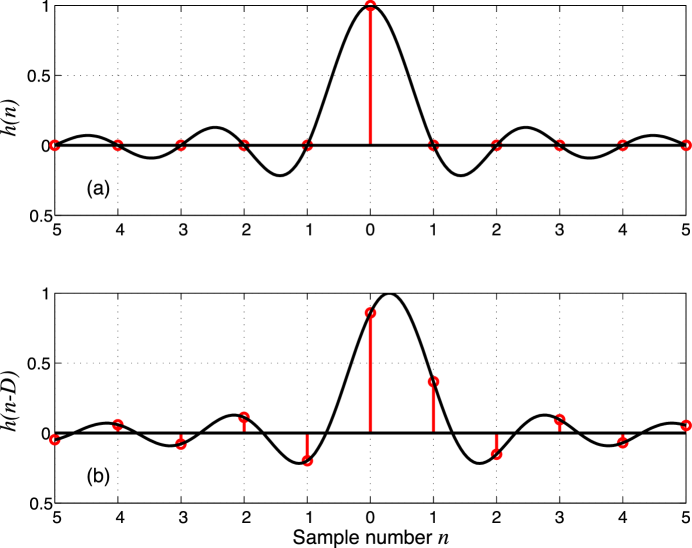
Figure 1: Sinc FIR filter kernel values (circles) with delay set to (a) $D=0$, and (b) $D=0.3$.

II.2 Truncated-sinc fractional-delay filters

The simplest finite-length approximation to the ideal delayed-sinc filter is obtained by truncating the kernel. Filtering by a truncated-sinc of kernel length $N$ can be written as

$$s_{N}(n-D)=\sum_{k=-\frac{N-1}{2}}^{\frac{N-1}{2}}s(n+k)\,\textrm{sinc}(D-k)\;\;\;\;\;\;\;\;\;{\rm(for\;odd}\;N).$$ (2)

In the following discussion we restrict ourselves to filters where $N$ is odd for simplicity.

Although for a given filter order $N$ the truncated-sinc is optimal in a least-squares sense Split , its frequency response is far from ideal (unity magnitude), exhibiting significant ripple even at low frequencies. This is unacceptable for TDI, where very high fidelity is required in the 1 mHz to 1 Hz measurement band. In fact, Ref. TintoPRD03 showed that truncated-sinc interpolation becomes sufficiently accurate only for very large $N$. Figure 2 shows the interpolation error versus $N$ for several filters, including the truncated-sinc. The interpolation error $\varepsilon$ is defined as the maximum difference of the filter’s frequency response and the ideal frequency response, ${\rm e}^{-i2\pi fD/f_{s}}$ for frequencies between 1 mHz and 1 Hz:

$$\varepsilon={\rm max}(|H(f)-{\rm e}^{-i2\pi fD/f_{s}}|_{1~{}{\rm mHz}\leq f\leq 1\;{\rm Hz}})$$ (3)

where $H(f)$ is the Fourier transform of $h(n)$. We used $D=0.5$, which is expected from theory to be the worst case. With truncated-sinc interpolation, $\varepsilon\approx 1/N$. Sampling at 10 Hz, this filter would require a kernel almost four months long, $N\gtrsim 10^{8}$, to achieve $\varepsilon<10^{-8}$. This means that two months of data at the beginning and end of each measurement period would be unusable.

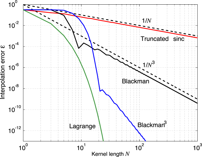
Figure 2: Comparison of interpolation error for four interpolation methods; truncated-sinc filter kernel, Blackman windowed-sinc filter kernel, Blackman³ windowed-sinc filter kernel, and Lagrange interpolation.

II.3 Windowed-sinc fractional-delay filters

The ripple in the frequency response of the truncated-sinc filter can be significantly reduced by windowing the filter,

$$s_{N}(n-D)=\sum_{k=-\frac{N-1}{2}}^{\frac{N-1}{2}}s(n+k)\,w(k)\,\textrm{sinc}(D-k),$$ (4)

where the window $w(k)$ goes smoothly to zero for $k=\pm(N-1)/2$, so that the endpoints are tapered to zero instead of abruptly truncated. Of several conventional windows Smith tested, the Blackman function

$$w_{b}(n) = 0.42+0.5\cos\left(\frac{\pi n}{N-1}\right)+0.08\cos\left(\frac{2\pi n}{N-1}\right)$$ (5)

was best, producing $\varepsilon<10^{-8}$ for $N\geq 345$ (see Fig. 2) corresponding to a loss of 14.4 seconds of data at the beginning and end of each measurement period. In comparison, the TDI combinations need several $L/c$ arm travel times, or at least 65 seconds, to gather enough data to cancel laser noise. As seen in Fig. 2, $\varepsilon\sim 1/N^{3}$ for Blackman windowed-sinc filters.

One simple modification to the Blackman windowed-sinc filter kernel is to apply the Blackman function more than once. Our tests showed that using $w_{b}^{3}(n)$ (applying the Blackman three times) produced $\varepsilon<10^{-8}$ for $N\geq 21$, corresponding to a loss of 1.1 seconds of data at the beginning and end of each measurement period.

II.4 Lagrange filter

A more accurate filter at low frequencies can be found by requiring a maximally flat frequency response at DC Split . This filter kernel is equal to the Lagrange polynomial  Koot96

$$h_{L}(n)=\prod_{\begin{subarray}{c}k=\frac{N-1}{2}\\ k\neq n\end{subarray}}^{\frac{N-1}{2}}\frac{t_{D}-k}{n-k},$$ (6)

where $t_{D}=\frac{N-1}{2}+D$. The Lagrange filter can be compared to filters in Section II.3 by expressing its kernel as a windowed-sinc function (Eq. 4), with the window

$$w_{L}(n)=\frac{\pi N}{\sin\pi t_{D}}{t_{D}\choose N}{N-1\choose n+(N-1)/2},$$ (7)

where the binomial coefficient is extended to non-integer arguments by the generalized factorial function (Gamma function) Gamma .

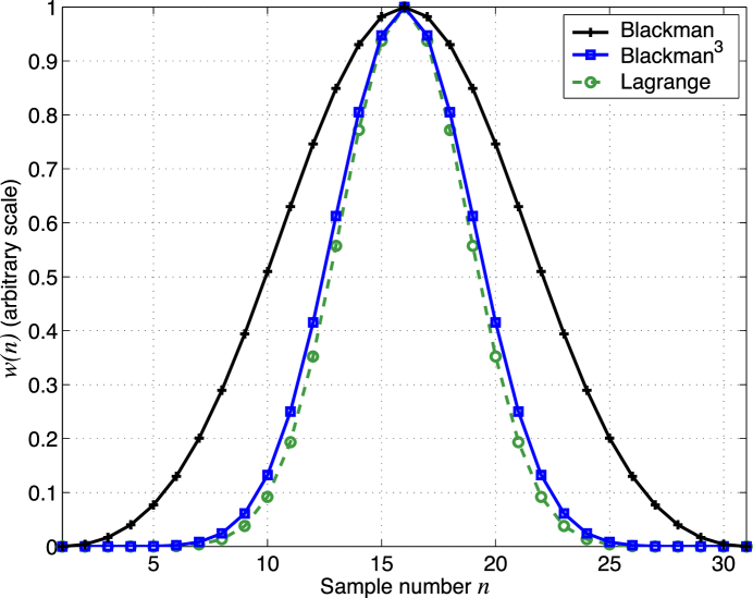
Figure 3: Blackman, Blackman³ and Lagrange windows with $N=31$.

Figure 3 shows the $w_{b}(n)$, $w_{b}^{3}(n)$ and $w_{L}(n)$ with $N=31$.

The performance of the Lagrange filter for this application is excellent, meeting the requirements with $N=15$ (1.5 seconds) as shown in Fig. 2. Although Lagrange interpolation is known to produce large spurious oscillations at the ends of the interpolation interval, this does not occur when the kernel is fully immersed in the signal. By accepting only data where the kernel is completely immersed, we obtain excellent performance at the expense of losing $N/2$ points at the beginning and end of each measurement period.

Lagrange interpolation is related also to the Thiran infinite-impulse-response (IIR) fractional-delay filter Split , which has nominally flat frequency response. The performance of the Thiran filter in our application is comparable to the Lagrange windowed-sinc FIR of the same order; but the latter is favored on grounds of simplicity, especially for time-dependent delays.

The filters were tested both by interpolating known analytic functions and interpolating bandlimited white noise. The bandlimited noise was generated with a sampling rate of 10 MHz and resampled at times $t=n/f_{s}$, $f_{s}=10$ Hz. The 10 Hz signal was delayed by $D$ samples and compared to the original 10 MHz signal resampled at times $t-D/f_{s}$. The test results agreed with the calculated fractional error shown in Fig. 2.

II.5 Further tests

We have characterized the error of fractional-delay filtering with fixed delays. In orbit, the delays will slowly vary due to the changing arm lengths, and so we also tested Lagrange filtering with varying delay. For this test, we generated a time series of white noise, bandlimited to 2.5 Hz and sampled at 10 Hz (oversampling factor of 2); we then used Lagrange filters of increasing order to interpolate the noise to the original sampling times shifted by delays ranging linearly in time from $D=-0.5$ to $D=0$ (no delay), during a period of $5\times 10^{5}$ seconds. This arrangement approximately simulates the slow variation in the LISA armlengths (which determine the TDI-mandated delays). Figure 4 shows spectra of the interpolation error, along with the spectrum of the original white noise. The required interpolation accuracy is achieved at all frequencies in the measurement band for $N\geq 16$ (window length of 1.6 s).

If the requirements become more stringent, for example due to increased laser frequency noise, it is easy to improve the performance to the desired level by increasing the length of the filter kernel. By setting the filter to $N=31$ (3 seconds in length at 10 Hz), $\varepsilon$ can be reduced to $1\times 10^{-15}$.

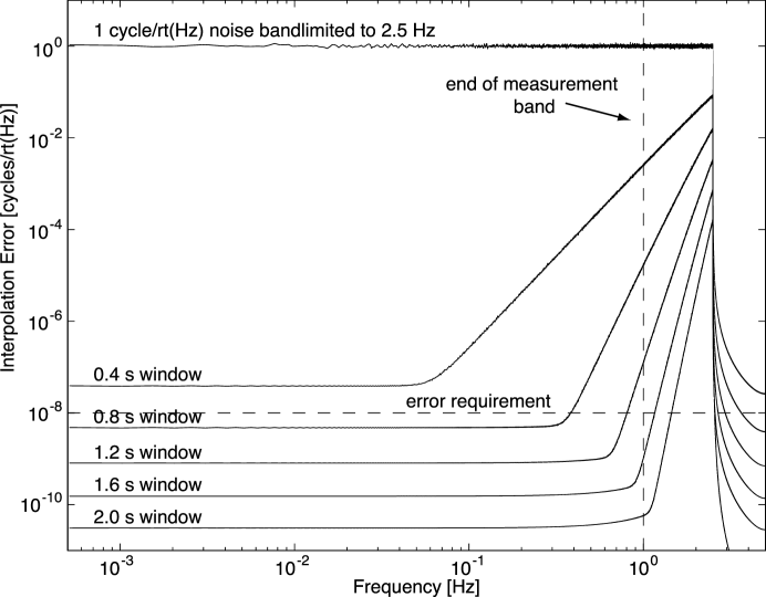
Figure 4: Amplitude spectral density of interpolation error for Lagrange filters, shown with the spectral density of the initial 2.5 Hz-bandlimited noise. Spectral density is estimated by a triangle-windowed, averaged periodogram.

III Implications for LISA

To illustrate the design simplifications enabled by high-precision interpolation, consider the simplest TDI combination–the Michelson combination $X(t)$ Tinto :

$$X(t)=[s_{21}(t)-s_{31}(t)]-[s_{21}(t-2L_{3}/c)-s_{31}(t-2L_{2}/c)].$$ (8)

where $s_{m1}$ is the phase measurement made at Spacecraft 1 of the light received from Spacecraft $m$, $L_{n}$ is the length of the arm opposite Spacecraft $n$, and we are assuming that the six LISA lasers are phase locked TintoPRD03 . The first two terms represent the optical phase of two arms of a Michelson interferometer, and the second two terms represent the same quantity with the specified delays.

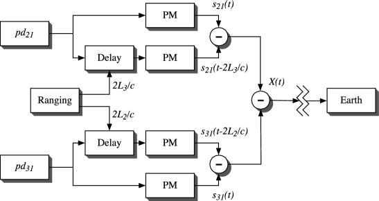
Figure 5: Real-time TDI, in which the delays must be known at the time of measurement, and the TDI combinations are computed before transponding to Earth. TDI combination $X(t)$ shown (Eq. 8).

The implementation of TDI based on timed triggering TintoPRD03 , which we designate “real-time TDI,” calls for all four terms in Eq. (8) to be explicitly measured, combined on-board, and sent to the Earth. This is illustrated in Fig. 5 for the measurement of $X(t)$ aboard Spacecraft 1. The blocks labeled $pd_{21}$ and $pd_{31}$ represent the radio-frequency beat signals from the photodiode outputs, containing laser frequency noise superimposed on the gravitational wave signal. The Ranging block represents the system that measures distances between spacecraft, and computes the delays $2L_{3}/c$ and $2L_{2}/c$ required to assemble $X(t)$. The telemetry inputs to the ranging blocks (not shown) contain ranging data measured on Spacecraft 1 and Spacecraft 2. Phase measurements are made by the phasemeter (PM) blocks. In Fig. 5, the phase signals are delayed electronically by the Delay blocks, which implement a variable delay as controlled by the ranging system. Equivalently, identical phase signals can be fed to two PM blocks, and the timing of the phase measurements can be set by adjustable triggers from the ranging system outputs. The final output $X(t)$ is free of laser frequency noise for fixed armlengths. For time-dependent armlengths, we expect ShaddockPRD03 that velocity-correcting or “second generation” TDI combinations will be required. They have roughly double the measurements of length-correcting or “first generation” TDI combinations such as that shown in Fig. 5.

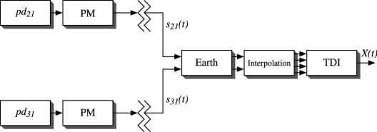
Figure 6: Post-processed implementation of TDI combination $X(t)$.

As we have demonstrated in this paper, the delayed phase measurements required for TDI can alternatively be inferred by interpolation from an equally-spaced sequence at a relatively low rate. This implementation is referred to as post-processed TDI and is shown in Figure 6. The elimination of the need for ranging knowledge at the time of measurement simplifies the implementation, as is evident comparing Figs. 5 and 6. Ranging information will still be needed as input to signal reconstruction, but it can be transmitted to Earth independently of the phasemeter signals. Alternatively, post-processed TDI can be implemented without explicit ranging by determining the delays using autocorrelations HellingsPRD01 , or by adjusting the delays in post-processing for minimum sensitivity to laser frequency variations. With post-processed TDI it is no longer necessary to synchronize the clocks on different spacecraft. Clock synchronization error can be corrected simply by time-shifting the data in post-processing. The decoupling of ranging from phase measurements and the removal of the need for clock synchronization allows reduction–or possibly elimination–of inter-spacecraft communications.

Post-processed TDI also allows complete flexibility in combining phasemeter signals. All the raw data are available for processing by any TDI algorithm, including ones not developed until after the data are in hand. The delays can be adjusted to optimize the suppression of laser frequency noise; by contrast, if there is an error in triggering in real-time TDI, noise is irrevocably added. Post-processed TDI simplifies the phase measurement hardware, allowing all possible TDI combinations to be constructed from one constant-rate phase measurement per photodetector.

A significant operating cost of LISA will be telemetry to Earth of science data. Real-time TDI requires one data stream per TDI combination. Post-processed TDI requires one data stream per phasemeter; more precisely, per phasemeter that does not have its output held fixed by a high-gain control system. We expect that post-processed TDI will require fewer telemetry signals than real-time TDI, but this depends on details of hardware design and on data requirements that are currently under consideration.

Other factors influencing overall telemetry costs are the data rate and number of bits per datum. The ultimate LISA data will have a signal bandwidth of 1 Hz and a dynamic range large enough to encompass both the largest expected gravitational wave signal (or perhaps the largest instrumental effect) and shot-noise limited sensitivity. Each output of the real-time TDI signal chain ($X(t)$ for example) will have essentially eliminated laser frequency noise before data are transponded to Earth, reducing the dynamic range requirement. A nominal datum size is 20 bits per sample. The data rate for each TDI combination is 2 samples/second, in keeping with the 1 Hz requirement and the Nyquist limit.

In comparison, post-processed TDI must transpond large laser frequency noise superimposed on the small gravitational wave signal. Larger dynamic range is required, perhaps 30 bits per sample. The sample rate for post-processed TDI is likely to be greater than 2 samples/second for two reasons. Firstly a larger sampling frequency may be needed to provide the more stringent anti-aliasing filtering needed when laser frequency noise is present. Secondly an oversampling factor may be needed for the interpolation procedure. The minimum sample rate imposed by post-processed TDI is still under study; our initial estimate is 10 samples/second (oversampling factor of 5) or less.

Although the interpolation algorithms presented here may not be optimal, they demonstrate the feasibility of post-processed TDI. They serve as a proof of principle, and provide guidance for the design of LISA with significant simplification in several respects over real-time TDI.

IV Acknowledgments

We thank John Armstrong for many useful discussions and for help with tests of the interpolation procedure. M.V. was supported by the LISA Mission Science Office at JPL. This research was performed at the Jet Propulsion Laboratory, California Institute of Technology, under contract with the National Aeronautics and Space Administration.

References

- (1) M. Tinto and J. W. Armstrong, “Cancellation of Laser Noise in an Unequal-Arm Interferometer Detector of Gravitational Radiation,” Phys. Rev. D 59, 102003 (1999); J. W. Armstrong, F. B. Estabrook, and M. Tinto, “Sensitivities of Alternate LISA Configurations,” Class. Quant. Grav. 18, 4059 (2001); M. Tinto, F. B. Estabrook, and J. W. Armstrong, “Time-Delay Interferometry for LISA,” Phys. Rev. D 65, 082003 (2002).
- (2) M. Tinto, D. A. Shaddock, J. Sylvestre, and J. W. Armstrong, “Implementation of time-delay interferometry for LISA,” Phys. Rev. D 67, 122003 (2003).
- (3) R. W. Hellings, “Elimination of clock jitter noise in spaceborne laser interferometers,” Phys. Rev. D 64, 022002 (2001).
- (4) T. I. Laakso et al., “Splitting the unit delay–tools for fractional delay filter design,” IEEE Signal Processing Magazine 13, 30 (1996).
- (5) C. E. Shannon, “Communication in the Presence of Noise,” Proceedings of the Institution of Radio Engineers, 37, 1, pp. 10 21 (1949).
- (6) S. W. Smith, The Scientist and Engineer’s Guide to Digital Signal Processing (California Technical Publishing, San Diego, CA, 1997).
- (7) P. J. Kootsookos and R. C. Williamson, “FIR Approximation of Fractional Sample Delay Systems,” IEEE Trans. on Circuits and Systems–II. Analog and Digital Signal Processing 43, 269 (1996).
- (8) W.H. Press, B. P. Flannery, S.A. Teukolsky, and W.T. Vetterling, Numerical Recipes in FORTRAN: The Art of Scientific Computing, 2nd ed. Cambridge, England: Cambridge University Press, pp. 206-209, 1992. E. W. Weisstein, “Binomial Coefficient,” From MathWorld, http://mathworld.wolfram.com/BinomialCoefficient.html .
- (9) D. A. Shaddock, M. Tinto, F. B. Estabrook, and J. W. Armstrong, Phys. Rev. D 68, 061303 (2003).