Static circularly symmetric perfect fluid solutions with an exterior BTZ metric.

Abstract

In this work we study static perfect fluid stars in $2+1$ dimensions with an exterior BTZ spacetime. We found the general expression for the metric coefficients as a function of the density and pressure of the fluid. We found the conditions to have regularity at the origin throughout the analysis of a set of linearly independent invariants. We also obtain an exact solution of the Einstein equations, with the corresponding equation of state $p=p(\rho)$, which is regular at the origin.

I Introduction

Researches realized before the discovery of the BTZ black hole solution BTZ , related with the behavior of extended sources, found that static circularly symmetric spacetime coupled to perfect fluids possess many unusual features not found in $3+1$ dimensions. For example, if the cosmological constant is not included, classical results show that there exist a universal mass, in the sense that all rotationally invariant structures in hydrostatic equilibrium have a mass that is proportional to the Planck mass, $m_{P}$, in 2+1 dimensions Cornish . In this case there is no black hole solution and the possibility of collapse is clearly forbidden. Nevertheless, the study of the structures with a mass $m$ and radius $R$, in hydrostatic equilibrium in anti-de Sitter gravity, leads to an upper bound on the ratio $m/R$ similar to the four dimensional case. This result shows that exist the possibility of collapse for matter distributions that have the ratio $m/R$ over the above upper bound Cruz . In this sense is possible to say that finite perfect fluid distributions in $2+1$ dimensional gravity with a negative cosmological constant has similar features comparable to the $3+1$ stars.

In $3+1$ dimensions it is relevant, since finite physical structures such as planet and stars exist, to obtain exact solutions of Einstein’s field equations for static spherically symmetric perfect fluid distribution which, in addition, satisfy physical considerations Finch98 . Recently, it has been presented different algorithms based on the choice of a single monotone function in order to generate all regular static spherically symmetric perfect fluid solutions of Einstein’s equations in $3+1$ dimensions Lake . The procedure to obtain the exact solutions of the Einstein equations in $2+1$ dimensions, corresponding to static circularly symmetric space-time coupled to perfect fluids, is straightforward via integration of the Einstein equations with cosmological constant as it was realized by A. García et al Garcia03 . Nevertheless, the exact solutions are presented in canonical coordinates, with a non direct physical interpretation. Only few exact solutions are known in curvature coordinates. Cornish et al Cornish found an exact solution for a $2+1$ dimensional star with a polytropic equation of state, and a flat exterior spacetime. Sá Sa consider the same equation of state but in an (anti)-de Sitter background, so the exterior correspond to a BTZ spacetime. In $3+1$ dimension the situation is very different and over one hundred solution have been found. See, for example Finch98 for a review. Recently, by means of computational program, the regularity of this solution at the origin has been studied in Delgaty . This study was realized using a set of linearly independent invariant found in Carminati . Previous works had found general conditions on the metric coefficients to fulfill the regularity at the origin Lake .

The purpose of this article is to investigate the regularity of a set of linearly independent invariants at the origin of the fluid distribution. We consider stars with an exterior BTZ space-time. In particular we use the method outlined in Garcia03 to obtain an exact solution of the Einstein’s equations in curvature coordinates. We choose the special case of density $\rho$ given by $\rho(r)=\rho_{0}(1-(r/a)^{2})$. We obtain the pressure $p$ as a function of $r$, which can be related with $\rho$ in order to obtain the corresponding equation of the state.

In Sec. II we briefly expose the methods of A. García et al to obtain solutions with an exterior BTZ metric. We obtain general expression for the metric coefficient in terms of the unknown functions $\rho(r)$ and $p(r)$. In sec. III we introduce the curvature invariants in order to analyze the conditions to obtain regularity of the invariants at the origin of the fluid distribution . In sec. IV we present a analytic solution, which will be tested with the procedure described above.

II Static circularly perfect fluid $2+1$ solution

The Einstein’s field equations are given by (with $G=1/8$ and $c=1$)

$$G_{\mu\nu}+\Lambda g_{\mu\nu}=\pi T_{\mu\nu}.$$ (1)

For a static circularly symmetric $2+1$ space-time the line element, in coordinates $\{r,t,\theta\}$, is given by

$$ds^{2}=-N^{2}(r)dt^{2}+\frac{dr^{2}}{G^{2}(r)}+r^{2}d\theta^{2}.$$ (2)

An straightforward integration of Einstein’s equations Garcia03 with negative cosmological constant, $\Lambda=-1/\ell^{2}$, and perfect fluid as source leads to the following expressions for the structural functions $G(r)$ and $N(r)$

$$G^{2}(r)=G^{2}_{0}+\frac{r^{2}}{\ell^{2}}-m(r),$$ (3)

where $m(r)$ is defined by the expression

$$m(r)=2\pi\int^{r}r\rho(r)dr,$$ (4)

and

$$N(r)=n_{0}+n_{1}\int^{r}\frac{r}{G(r)}dr,$$ (5)

where $n_{0}$ and $n_{1}$ are integrating constants. The energy density, $\rho(r)$, is related to fluid pressure by means of some unknown state equation $p=p(\rho)$.

For these finite distributions the exterior spacetime correspond to a BTZ background, described by the metric

$$ds^{2}=-(-M+\frac{r^{2}}{\ell^{2}})dt^{2}+\frac{dr^{2}}{(-M+\frac{r^{2}}{\ell^{2}})}+r^{2}d\theta^{2},$$ (6)

which posses an event horizon at $r=\ell\sqrt{M}$. Of course, the surface of our distribution is located at $r=a>\ell\sqrt{M}$. Therefore, we must give the conditions on the junction surface, $r=a$, for the interior and exterior metrics Israel66 . Lubo et al have showed in Lubo , that the equality of the induced metric on the junction surface implies the continuity of the interior and exterior metric, i. e., $g^{in}_{\mu\nu}\mid_{r=a}=g^{ext}_{\mu\nu}\mid_{r=a}$, where $\mu,\nu\in(t,r,\theta)$. The equality of the extrinsic curvature with respect to the two space-time geometries reduces to require the continuity of some of the metric component derivatives, i. e., $[\partial_{r}g^{in}_{\mu\nu}]_{r=a}=[\partial_{r}g^{ext}_{\mu\nu}]_{r=a}$, where $\mu,\nu\in(t,\theta)$.

The first matching condition yields to the following equations for $g_{00}$ and $g_{11}$, respectively:

$$N^{2}(a)=-M+\frac{a^{2}}{\ell^{2}},$$ (7)

and

$$G^{2}(a)=-M+\frac{a^{2}}{\ell^{2}}.$$ (8)

Note that above condition on $g_{22}$ is automatically satisfied. This two last equations leads to a relation that we use below:

$$N^{2}(a)=G^{2}(a)=-M+\frac{a^{2}}{\ell^{2}}.$$ (9)

From equation (3) and (8), we can find the value of $G^{2}_{0}$

$$G^{2}_{0}=m(a)-M$$ (10)

At the origin the structural function goes to: $G^{2}\rightarrow G^{2}_{0}$ and $N^{2}\rightarrow n^{2}_{0}$. With the change of variables: $n_{0}t\rightarrow T$ and $G^{-1}_{0}r\rightarrow R$, we obtain that near the origin $ds^{2}=-dT^{2}+dR^{2}+R^{2}(G^{-2}_{0}d\theta^{2})$. In order to avoid an angular lack or an angular excess (elementary flatness), $G^{-2}_{0}>1$ or $G^{-2}_{0}<1$, respectively, we choose $G^{-2}_{0}=1$. With this argument the structural function, $G^{2}(r)$, is given by

$$G^{2}(r)=1+\frac{r^{2}}{\ell^{2}}-m(r),$$ (11)

Note that $G^{2}(r)>0$ within the fluid distribution since $a>\ell\sqrt{M}$. This imposes restrictions upon the value of the density at the origin.

The second matching condition on $g_{22}$ is automatically satisfied, but on $g_{00}$ become

$$N(a)[\partial_{r}N(r)]_{r=a}=\frac{a}{\ell^{2}},$$ (12)

The left hand side can be evaluated from (5) and (9), obtaining the value of the integrating constant $n_{1}$

$$n_{1}=\frac{1}{\ell^{2}}.$$ (13)

On the other hand, an evaluation of the pressure in the Einstein’s equation Garcia03 leads to

$$\pi p(r)=\frac{1}{N(r)}[n_{1}G(r)-\frac{N(r)}{\ell^{2}}].$$ (14)

In our case, from (13) we have

$$\pi p(r)=\frac{1}{\ell^{2}N(r)}[G(r)-N(r)].$$ (15)

This showed that the geometrical condition find in (9) yields to the condition to pressure zero at $r=a$. So, it allow us to write $N(r)$ in the following form

$$N(r)=\frac{1}{1+\pi\ell^{2}p(r)}G(r)\equiv f(r)G(r),$$ (16)

where the condition $f(r=a)=1$ is satisfied.

The metric (2) with $G(r)$ and $N(r)$ given by equations (11) and (16) respectively, represents the space-time corresponding to the static circularly symmetric $2+1$ solutions of Einstein’s equations with negative cosmological constant for a given perfect fluid.

III Regularity of invariants

We have demanded that the interior metric satisfy the regularity condition imposed by elementary flatness. Nevertheless, this condition by no means guarantees regularity. A spacetime describing the geometry inside a physical fluid distribution must be regular at the origin ($r=0$). In $3+1$ dimensions Lake and Musgrave have found in Lake the necessary and sufficient conditions for securing the regularity at the origin of a spherically symmetric static spacetime in terms of the metric coefficients, when curvature coordinates are used. These conditions have been derived demanding the regularity at the origin of four algebraically independent second order curvature invariants. In our case, we will examine the regularity of this set curvature invariants at the origin for general spacetime describing a perfect fluid within a finite fluid distribution, with a boundary which matched with the BTZ metric. Since $G(r)$ and $N(r)$ can be expressed in terms of the pressure and the density, we obtain that the regularity at the origin implies conditions on the pressure and density. The set of non-vanishing invariants are $R=g^{ab}R_{ab}$, $R_{1}\equiv S^{b}_{a}S^{a}_{b}/4$, $R_{2}\equiv-S^{b}_{a}S^{c}_{b}S^{a}_{c}/8$, and $R_{3}\equiv S^{b}_{a}S^{c}_{b}S^{d}_{c}S^{a}_{d}/16$, where $S^{b}_{a}$ is the trace-free Ricci tensor given by $S^{b}_{a}=R^{b}_{a}-\delta^{b}_{a}R/4$, and $R$ is the Ricci scalar.

Using the GRTensor II program we found the following expressions for above invariants in terms of $G^{2}(r)$, the pressure $p(r)$ and its derivatives.

$$R=-2\left[\left(\frac{(G^{2}(r))^{\prime}}{r}\right)-\frac{\pi\ell^{2}G^{2}(r)}{(1+\pi\ell^{2}p(r))}\left(\frac{p^{\prime}}{r}\right)+\frac{w(r)}{(1+\pi\ell^{2}p(r))^{2}}\right],$$ (17)

$$R1 = \left[\left(\frac{(G^{2}(r))^{\prime}}{4r}\right)-\frac{\pi\ell^{2}G^{2}(r)}{(1+\pi\ell^{2}p(r))}\left(\frac{p^{\prime}}{4r}\right)\right]^{2}+\frac{\pi^{2}\ell^{4}G^{4}(r)}{(1+\pi\ell^{2}p(r))^{2}}\left(\frac{p^{\prime}}{4r}\right)^{2}$$ (18)

$$-\frac{w(r)}{2(1+\pi\ell^{2}p(r))^{2}}\left[\left(\frac{(G^{2}(r))^{\prime}}{4r}\right)-\frac{\pi\ell^{2}G^{2}(r)}{(1+\pi\ell^{2}p(r))}\left(\frac{p^{\prime}}{4r}\right)\right]+\frac{3w^{2}(r)}{16(1+\pi\ell^{2}p(r))^{4}},$$

$$R2 = \left[\left(\frac{(G^{2}(r))^{\prime}}{4r}\right)-\frac{\pi\ell^{2}G^{2}(r)}{(1+\pi\ell^{2}p(r))}\left(\frac{p^{\prime}}{4r}\right)\right]^{3}$$ (19)

$$-\frac{3w(r)}{4(1+\pi\ell^{2}p(r))^{2}}\left(\left[\left(\frac{(G^{2}(r))^{\prime}}{4r}\right)-\frac{\pi\ell^{2}G^{2}(r)}{(1+\pi\ell^{2}p(r))}\left(\frac{p^{\prime}}{4r}\right)\right]^{2}\right.$$

$$\left.-\frac{\pi^{2}\ell^{4}G^{4}(r)}{(1+\pi\ell^{2}p(r))^{2}}\left(\frac{p^{\prime}}{4r}\right)^{2}\right)+\frac{3w^{2}(r)}{16(1+\pi\ell^{2}p(r))^{4}}$$

$$\times\left[\left(\frac{(G^{2}(r))^{\prime}}{4r}\right)-\frac{\pi\ell^{2}G^{2}(r)}{(1+\pi\ell^{2}p(r))}\left(\frac{p^{\prime}}{4r}\right)\right]+\frac{w^{3}(r)}{64(1+\pi\ell^{2}p(r))^{6}},$$

$$R3 = \left[\left(\left(\frac{(G^{2}(r))^{\prime}}{4r}\right)-\frac{\pi\ell^{2}G^{2}(r)}{(1+\pi\ell^{2}p(r))^{2}}\left(\frac{p^{\prime}}{4r}\right)\right)^{4}-\frac{2\pi^{4}\ell^{8}G^{8}(r)}{(1+\pi\ell^{2}p(r))^{4}}\left(\frac{p^{\prime}}{4r}\right)^{4}\right]$$ (20)

$$-\frac{w(r)}{(1+\pi\ell^{2}p(r))^{2}}\left[\left(\frac{(G^{2}(r))^{\prime}}{4r}\right)-\frac{\pi\ell^{2}G^{2}(r)}{(1+\pi\ell^{2}p(r))}\left(\frac{p^{\prime}}{4r}\right)\right]^{3}$$

$$+\frac{3w^{2}(r)}{8(1+\pi\ell^{2}p(r))^{4}}\left[\left(\left(\frac{(G^{2}(r))^{\prime}}{4r}\right)-\frac{\pi\ell^{2}G^{2}(r)}{(1+\pi\ell^{2}p(r))^{2}}\left(\frac{p^{\prime}}{4r}\right)\right)^{2}-\frac{\pi^{2}\ell^{4}G^{4}(r)}{(1+\pi\ell^{2}p(r))^{2}}\left(\frac{p^{\prime}}{4r}\right)^{2}\right]$$

$$-\frac{w^{3}(r)}{64(1+\pi\ell^{2}p(r))^{6}}\left[\left(\frac{(G^{2}(r))^{\prime}}{4r}\right)-\frac{\pi\ell^{2}G^{2}(r)}{(1+\pi\ell^{2}p(r))}\left(\frac{p^{\prime}}{4r}\right)\right]+\frac{3w^{4}(r)}{256(1+\pi\ell^{2}p(r))^{8}},$$

Where $w(r)$ is given by

$$w(r) = ((1+\pi\ell^{2}p(r))^{2}(G^{\prime}(r))^{2}-3\pi\ell^{2}G(r)(1+\pi\ell^{2}p(r))G^{\prime}(r)p^{\prime}(r)$$ (21)

$$+G(r)((1+\pi\ell^{2}p(r))^{2}(G^{\prime\prime}(r))+\pi\ell^{2}G(r)(2\pi\ell^{2}(p^{\prime}(r))^{2}-(1+\pi\ell^{2}p(r))p^{\prime\prime}(r)))).$$

From the inspection of the invariants it is straightforward to find the conditions to assure regularity within the fluid distribution. The regularity of the functions $G^{2}(r)$, $\frac{(G^{2}(r))^{\prime}}{r}=\frac{2}{\ell^{2}}-2\pi\rho$ and $G(r)^{\prime\prime}$ is guarantee if and only if $\rho(r)$ is regular within the fluid distribution. Clearly, the pressure will be regular if and only if the structural function, $N(r)$, will not be zero within distribution (see equation (15)). This requirement is satisfies at the origin, since, when $r\rightarrow 0$, $N\rightarrow n_{0}$. On the other hand, from the Tolman-Oppenheimer-Volkov hidrostatic equilibrium equation, given by

$$\frac{1}{r}\frac{dp}{dr}\equiv\frac{p^{\prime}}{r}=-\frac{1}{G^{2}(r)}\left(\pi p+\frac{1}{\ell^{2}}\right)(p+\rho),$$ (22)

we find that $p^{\prime}$ and $p^{\prime\prime}$ are regular if and only if $\rho$ is regular at the origin. Thus for $2+1$ finite fluid distributions the invariants are regular if $\rho$ is regular.

IV Exact and regular solution for $\rho(r)=\rho_{0}(1-(r/a)^{2})$

We choose the following density function, which is finite by construction in $r=0$ ($\rho(0)=\rho_{0}$), as well as is decreasing (up to its zero value) when $r\rightarrow a$

$$\rho(r)=\rho_{0}(1-(r/a)^{2}).$$ (23)

Thus, $m(r)=m\frac{r^{2}}{a^{2}}(2-\frac{r^{2}}{a^{2}})$, where $m\equiv m(r=a)=\frac{\pi a^{2}\rho_{0}}{2}$. Therefore, the structural functions $G^{2}(r)$ and $N(r)$ are given by

$$G^{2}(r)=1-\frac{(2m-\frac{a^{2}}{\ell^{2}})}{a^{2}}r^{2}+\frac{m}{a^{4}}r^{4},$$ (24)

and

$$N(r)=\frac{a^{2}}{2\ell^{2}\sqrt{m}}\ln\left[\frac{2m((\frac{r}{a})^{2}-1)+2\sqrt{m}G(r)+\frac{a^{2}}{\ell^{2}}}{2\sqrt{m}G(a)+\frac{a^{2}}{\ell^{2}}}e^{\frac{2\ell^{2}\sqrt{m}G(a)}{a^{2}}}\right].$$ (25)

Clearly, the both matching condition are satisfies. Evaluating the pressure from the expression (15), we obtain

$$\pi\ell^{2}p(r)=\frac{2\sqrt{m}\sqrt{1-(2m-\frac{a^{2}}{\ell^{2}})(\frac{r}{a})^{2}+m(\frac{r}{a})^{4}}}{\ln\left[\frac{2m((\frac{r}{a})^{2}-1)+2\sqrt{m}(1-(2m-\frac{a^{2}}{\ell^{2}})(\frac{r}{a})^{2}+m(\frac{r}{a})^{4})+\frac{a^{2}}{\ell^{2}}}{2\sqrt{m}G(a)+\frac{a^{2}}{\ell^{2}}}e^{\frac{2\ell^{2}\sqrt{m}G(a)}{a^{2}}}\right]}-1.$$ (26)

Since the coordinated $r$ can be written in terms of $\rho$ like $r^{2}=a^{2}(1-\rho/\rho_{0})$, we can re-define

$$G^{2}(r)\rightarrow\tilde{G}^{2}(\rho)=\tilde{G}^{2}(0)+\frac{\rho}{\rho_{0}}\left(\frac{a^{2}}{\ell^{2}}+m\frac{\rho}{\rho_{0}}\right),$$ (27)

where $\tilde{G}^{2}(0)=1+\frac{a^{2}}{\ell^{2}}-m$. The state equation is given by

$$\pi\ell^{2}p(\rho)=\frac{2\sqrt{m}\tilde{G}(\rho)}{\ln\left[\frac{2\sqrt{m}\tilde{G}(\rho)+\frac{a^{2}}{\ell^{2}}-2m\frac{\rho}{\rho_{0}}}{2\sqrt{m}\tilde{G}(0)+\frac{a^{2}}{\ell^{2}}}e^{\frac{2\ell^{2}\sqrt{m}\tilde{G}(0)}{a^{2}}}\right]}-1.$$ (28)

The metric can be expressed completely in terms of the function $\rho$, which assures that this is totally regular inside the distribution

$$ds^{2}=-\frac{\tilde{G}^{2}(\rho)}{(1+\pi\ell^{2}p(\rho))^{2}}dt^{2}+\frac{dr^{2}}{\tilde{G}^{2}(\rho)}+a^{2}(1-\rho/\rho_{0})d\theta^{2}.$$ (29)

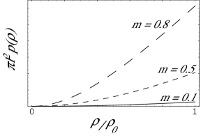
Figure 1: State equation $\pi\ell^{2}p(\rho)$ v/s $\rho/\rho_{0}$ for $\frac{a^{2}}{\ell^{2}}=0.005m$

The curvature invariants, expressed in terms of the pressure and the density of the perfect fluid, are regular in the origin of the distribution, as we have shown

$$R=-\frac{6}{\ell^{2}}-2\pi(2p(\rho)-\rho),$$ (30)

$$R1=\frac{1}{16\ell^{4}}[(3+\pi\ell^{2}(2p(\rho)-\rho))(1-\pi\ell^{2}(2p(\rho)+3\rho))],$$ (31)

$$R2 = \frac{1}{64\ell^{6}}[3-3\pi\ell^{2}(2p(\rho)+\rho)+3\pi^{2}\ell^{4}(4p^{2}(\rho)-4\rho p(\rho)+3\rho^{2})$$ (32)

$$-\pi^{3}\ell^{6}(8p^{3}(\rho)-12\rho p^{2}(\rho)+6\rho^{2}p(\rho)+3\rho^{3})],$$

$$R3 = \frac{1}{256\ell^{8}}[3+\pi\ell^{2}(16\pi^{3}\ell^{6}+32\pi^{2}\ell^{4}p^{3}(\rho)(1+\pi\ell^{2}\rho)+24\pi\ell^{2}p^{2}(\rho)(1+\pi\ell^{2}\rho)^{2}$$ (33)

$$+8p(\rho)(1+\pi\ell^{2}\rho)^{3}+\rho(\pi\ell^{2}\rho(18+\pi\ell^{2}\rho(3\pi\ell^{2}\rho-4))-4))].$$

V Conclusions

We have presented a method to generate exact and regular perfect fluid solutions of spherically symmetric static stars with an exterior BTZ spacetime. The regularity conditions have been established by means of a set of invariants, which can be expressed in terms of the density, $\rho(r)$, and the pressure, $p(r)$. We have found that for a static perfect fluid distribution in hydrostatic equilibrium the interior solutions are regular at the origin if $\rho$ is regular.

Starting from a function of density $\rho(r)=\rho_{0}(1-r^{2}/a^{2})$, which is, by construction, regular at the origin and decreasing up to zero in $r=a$, we have found an exact and regular interior solution in the coordinates $(t,r,\theta)$, deriving its corresponding equation of state. Finally, the set of independent invariants has been evaluated showing its regularity at the origin. Its is direct to see that at the surface junction the invariants take the values corresponding to the invariants of the BTZ spacetime.

References

(1) M. Bañados, C. Teitelboim and J. Zanelli, Phys. Rev. Lett.69 (1992) 1849.
(2) N. J. Cornish and N. E. Frankel, Phys. Rev.D
43 (1991) 2555.
(3) N. Cruz and J. Zanelli, Class. Quantum. Grav.12, (1995) 975.
(4) M. R. Finch and J. E. F. Skea, A Review of the relativistic
static fluid sphere, (preprint available on the World Wide Web at
http://edradour.symbcomp.uerj.br/pubs.html)
(5) K. Lake and P. Musgrave Gen. Rel. Grav.26 (1994) 917; S. Rahman and
M. Visser, Class. Quantum. Grav.19, (2002) 935.
(6) A. Garcia and C. Campuzano, Phys. Rev.D67, (2003) 064014.
(7) R.Adler, M. Bazin and M. Schiffer, Introducction to General
Relativity 2nd Ed. McGraw-Hill, N. Y., 1975.