Gravitational Waves from Chaotic Dynamical System

Abstract

To investigate how chaos affects gravitational waves, we study the gravitational waves from a spinning test particle moving around a Kerr black hole, which is a typical chaotic system. To compare the result with those in non-chaotic dynamical system, we also analyze a spinless test particle, which orbit can be complicated in the Kerr back ground although the system is integrable. We estimate the emitted gravitational waves by the multipole expansion of a gravitational field. We find a striking difference in the energy spectra of the gravitational waves. The spectrum for a chaotic orbit of a spinning particle, contains various frequencies, while some characteristic frequencies appear in the case of a spinless particle.

I Introduction

The current ground-base gravitational wave detectors such as LIGO, TAMA300, GEO600 and VIRGO  LIGO ; TAMA ; GEO ; VIRGO are now starting the “science run” and the laser space antenna for gravitational waves(LISA) LISA may operate in the near future. Gravitational waves will bring us various new information about relativistic astrophysical objects. If we will detect gravitational waves and compare them with theoretical templates, we may be able to determine a variety of astrophysical parameters of the sources such as their direction, distance, masses, spin, and so on. The direct observation of gravitational waves could resolve strong-gravitational phenomena such as a black hole formation. Furthermore, we may be able not only to verify the theory of gravity but also to find new information or to recover new physics at high density or high energy region. Therefore we need to make theoretical templates of gravitational waves from various astrophysical objects and phenomena to extract useful information from gravitational waves.

There are a lot of astrophysical objects and phenomena as gravitational wave sources, e.g., a closed binary system or a supernova explosion. Many attempts to study their templates have been done so far. In this paper, we particularly focus on a gravitational waves form a chaotic dynamical system. It is motivated as follows. Chaos appears universally in nature and it is expected to explain various nonlinear phenomena. Because chaos indicates unpredictability of motion of objects, it comes into a question whether or not that it is possible to extract useful information from a chaotic system. Many studies have been made on chaos in mechanics and astrophysics since the research on the three-body problem by Poncaré. It is also important to study chaos in general relativity because the Einstein equations are nonlinear. Many authors have reported chaos in general relativity  Hobill ; Barrow ; Conto ; Dettmann ; Yust ; Karas ; Varvoglis ; Bombelli ; Moeckel ; Sota ; Suzuki ; Suzuki2 ; Suzuki3 ; Mich ; Seme ; Levin ; Schnittman ; Cornish . As for a realistic astrophysical object, there has been a discussion whether or not chaos occurs in a compact binary system Levin ; Schnittman ; Cornish . It seems that there is not enough time in a compact binary for chaos to occur even in a non-integrable system. Then we may not have so far any concrete example of general relativistic chaos for a realistic situation. However, we believe that it is necessary to study chaos in general relativity. Because chaos will occur in a realistic strong gravitational field described by general relativity.

In this paper, we study some observational feature of chaos in general relativistic dynamical system. We focus on gravitational waves from a chaotic dynamical system. As a model of a chaotic dynamical system, we adopt a spinning test particle around a rotating black hole. It mimics a model of compact objects orbiting around a super massive black hole. Recent observations support the existence of such massive black holes and LISA will be sensitive to the gravitational wave from such systems. As for a background spacetime, we assume the Kerr metric since such a supermassive black hole is usually rotating. The previous works Suzuki ; Seme revealed that orbits of a spinning test particle around a black hole can be chaotic due to the spin-orbit coupling. We evaluate the gravitational waves emitted from this system by using multipole expansion of a gravitational field. Landau ; Mathews ; Kip .

Carter showed Cart that the equations of motion for a spinless particle are integrable. After his work, Johnston discovered that motion for some initial parameters, the particle motion can be very complicated as if chaos occurred, although the system is integrable John . Then we also analyze such non-chaotic but complicated orbital motion to clarify whether or not chaos is essential in our results. We compare the wave forms and the energy spectra of the gravitational waves from both chaotic and nonchaotic systems and analyze the effects of chaos on gravitational waves.

This paper is organized as follows. In Sec. II we shall briefly review the basic equations of both a spinless particle and a spinning particle in relativistic spacetime, a supplementary condition, and some constants of motion. Specifying the background spacetime to be the Kerr metric, we show our results in Sec. III. Summary and some remarks follow in Sec. IV.
Throughout this paper we use units $c=G=1$. Our notation including the signature of the metric follows that of Misner Thorne and Wheeler(MTW) MTW .

II Basic equations for a test particle

First we explain our system more precisely.

II.1 Background spacetime

We consider the Kerr metric as a background spacetime. In the Boyer-Lindquest coordinates, it is given by

$$ds^{2}= -\Big{(}1-\frac{2Mr}{\Sigma}\Big{)}dt^{2}-\frac{4Mar\sin^{2}\theta}{\Sigma}dtd\phi$$

$$+ \frac{\Sigma}{\Delta}dr^{2}+\Sigma d\theta^{2}+\sin^{2}\theta\Big{(}r^{2}+a^{2}+\frac{2Ma^{2}r\sin^{2}\theta}{\Sigma}\Big{)}d\phi^{2},$$ (1)

where

$$\Sigma =r^{2}+a^{2}\cos^{2}\theta,$$ (2)

$$\Delta =r^{2}-2Mr+a^{2},$$ (3)

and $M$ and $a$ are the mass of a black hole and its angular momentum, respectively.

II.2 A spinless test particle

In this subsection, we summarize the equations of motion for a spinless test particle. It is well known that a spinless test particle moves along geodesic

$$\frac{d^{2}x^{\mu}}{d\tau^{2}}+\Gamma^{\mu}_{\nu\rho}\frac{dx^{\nu}}{d\tau}\frac{dx^{\rho}}{d\tau}=0,$$ (4)

where $\tau$ is an affine parameter of the orbit. In a stationary axisymmetric spacetime, a spinless particle has two constants of motion; the Energy $E$ and the $z$-component of the angular momentum $L_{z}$. The particle’s rest mass $\mu$ is also constant. Carter discovered third constant of motion and showed that the system is integrable Cart . Eq. (4) is reduced to a set of the differential equations as

$$\Sigma\frac{d\theta}{d\tau}=\pm\sqrt{\Theta},$$ (5)

$$\Sigma\frac{dr}{d\tau}=\pm\sqrt{R},$$ (6)

$$\Sigma\frac{d\phi}{d\tau}=-\Big{(}aE-\frac{L_{z}}{\sin^{2}\theta}\Big{)}+\frac{a}{\Delta}P,$$ (7)

$$\Sigma\frac{dt}{d\tau}=-a(aE\sin^{2}\theta-L_{z})+\frac{r^{2}+a^{2}}{\Delta}P,$$ (8)

where

$$\Theta(\theta) =C-\cos^{2}\theta\Big{\{}a^{2}(1-E^{2})+\frac{L_{z}^{2}}{\sin^{2}\theta}\Big{\}},$$ (9)

$$P(r) =E(r^{2}+a^{2})-aL_{z},$$ (10)

$$R(r) =P^{2}-\Delta\{r^{2}+(L_{z}-aE)^{2}+C\},$$ (11)

and $C$ is a constant discovered by Carter and called the Carter constant. Note that because of the presence of the Carter constant, the orbits of a particle will never be chaotic.

II.3 A spinning test particle

The equations of motion for a spinning test particle in a relativistic spacetime were first derived by Papapetrou Papa and then reformulated by Dixon Dix . They used the pole-dipole approximation, in which multipole moments of an object higher than a mass monopole and a spin dipole are ignored in the limit of a point particle. The set of equations is given as

$$\frac{dx^{\mu}}{d\tau}=v^{\mu},$$ (12)

$$\frac{Dp^{\mu}}{d\tau}=-\frac{1}{2}{R^{\mu}}_{\nu\rho\sigma}v^{\nu}S^{\rho\sigma},$$ (13)

$$\frac{DS^{\mu\nu}}{d\tau}=2p^{[\mu}v^{\nu]},$$ (14)

where $\tau,v^{\mu},p^{\mu}$ and $S^{\mu\nu}$ are an affine parameter of the orbit, the four-velocity of a particle, the momentum, and the spin tensor, respectively. $p^{\mu}$ deviates from a geodesic due to the coupling of the Riemann tensor with the spin tensor. We also need an additional condition which gives a relation between $p^{\mu}$ and $v^{\mu}$. We adopt the condition formulated by Dixon Dix

$$p_{\mu}S^{\mu\nu}=0.$$ (15)

This condition consistently determines the cetnter of mass in the present system. Using Eq (15), we can determine the relation between $p^{\mu}$ and $v^{\mu}$ explicitly as

$$v^{\mu}=N\Big{[}u^{\mu}+\frac{1}{2\mu^{2}\delta}R_{\nu\lambda\rho\sigma}S^{\mu\nu}u^{\lambda}S^{\rho\sigma}\Big{]},$$ (16)

where

$$\delta=1+\frac{1}{4\mu^{2}}R_{\alpha\beta\gamma\sigma}S^{\alpha\beta}S^{\gamma\sigma},$$ (17)

and $N$ is a normalization constant, which is fixed by a choice of the affine parameter $\tau$ as we will explicitly show it later. $u^{\mu}\equiv p^{\mu}/\mu$ is a unit vector parallel to the four-momentum $p^{\mu}$, where the mass of the particle $\mu$ is defined by

$$\mu^{2}=-p_{\mu}p^{\mu}.$$ (18)

To make clear the freedom of this system, we have to check the conserved quantities. Regardless of the symmetry of the background spacetime, it is easy to show that $\mu$ and the magnitude of spin $S$ defined by

$$S^{2}\equiv\frac{1}{2}S_{\mu\nu}S^{\mu\nu},$$ (19)

are constants of motion. If a background spacetime possesses some symmetry described by a Killing vector $\xi^{\mu}$,

$$C_{\xi}\equiv\xi^{\mu}p_{\mu}-\frac{1}{2}\xi_{\mu;\nu}S^{\mu\nu}$$ (20)

is also conserved Dix . For a spacetime with both axial and timelike Killing vectors such as Kerr spacetime, we have two conserved quantities, i.e., the Energy $E$ and the $z$-component of the total angular momentum $J_{z}$ of a spinning particle.

For numerical reasons, we rewrite our basic equations as follows. Following the appendix in Suzuki , we write down the equations by use of a spin vector

$$S_{\mu}\equiv-\frac{1}{2}\epsilon_{\mu\nu\rho\sigma}u^{\nu}S^{\rho\sigma},$$ (21)

where $\epsilon^{\mu\nu\rho\sigma}$ is the Levi-Civita tensor. The basic equations are now

$$\frac{dx^{\mu}}{d\tau} =v^{\mu},$$ (22)

$$\frac{Dp^{\mu}}{d\tau} =\frac{1}{\mu}{R^{*\mu}}_{\nu\rho\sigma}v^{\nu}S^{\rho}p^{\sigma},$$ (23)

$$\frac{DS^{\mu}}{d\tau} =\frac{1}{\mu^{3}}p^{\mu}{R^{*}}_{\nu\rho\sigma\gamma}S^{\nu}v^{\rho}S^{\sigma}p^{\gamma},$$ (24)

where

$${R^{*}}_{\mu\nu\rho\sigma}\equiv\frac{1}{2}{R_{\mu\nu}}^{\alpha\beta}\epsilon_{\alpha\beta\rho\sigma}.$$ (25)

Eq. (15) is also rewritten

$$p_{\nu}S^{\nu}=0.$$ (26)

By this condition, the relation between $p^{\mu}$ and $v^{\mu}$ is determined as follow :

$$v^{\mu}=u^{\mu}+\frac{1}{\mu^{2}}{{}^{*}R^{*\mu}}_{\nu\rho\sigma}S^{\nu}S^{\rho}u^{\sigma},$$ (27)

where

$${{}^{*}R^{*}}_{\mu\nu\rho\sigma}\equiv\frac{1}{2}\epsilon_{\mu\nu\alpha\beta}{R^{*\alpha\beta}}_{\rho\sigma}.$$ (28)

We fix the affine parameter $\tau$ using the condition $v^{\mu}u_{\mu}=-\delta$. This gives $N$ as

$$N=1+\frac{1}{\mu^{4}}{{}^{*}R}^{*}_{\alpha\beta\mu\nu}S^{\alpha}p^{\beta}S^{\mu}p^{\nu},$$ (29)

Our conserved quantities are also rewritten as

$$S^{2}=S_{\mu}S^{\mu},$$ (30)

$$C_{\xi}=\xi^{\mu}p_{\mu}-\frac{1}{2\mu}\xi_{\mu;\nu}\epsilon^{\mu\nu\rho\sigma}p_{\rho}S_{\sigma}.$$ (31)

III Numerical results

In this section, we show our numerical results for the orbital motion of a test particle, and the wave forms and the energy spectra of the emitted gravitational waves. To analyze chaotic behavior of a test particle, we use the Poincaré map and the Lyapunov exponent. To draw the Poincaré map, we adopt the equatorial plane ($\theta=\pi/2$) as a Poncaré section and plot the point ($r$, $v^{r}$) when the particle crosses the Poincaré section with $v^{\theta}<0$. If the motion is not chaotic, the plotted points will form a closed curve in the two dimensional $r$-$v^{r}$ plane, because a regular orbit will move on a torus in the phase space and the curve is a cross section of the torus. If the orbit is chaotic, some of these tori will be broken and the Poincaré map does not consist of a set of closed curves but the points will be distributed randomly in the allowed region. From the distribution of the points, we can judge whether or not the motion is chaotic.

III.1 Motion of a test particle

III.1.1 a spinless particle

As we see in Sec II.2, the equations of the motion of a spinless particle are integrable because of the existence of the Carter constant. That is chaos does not occur. But Johnston found that the orbits of a spinless particle can be complicated as if chaos occurred John . Integrating numerically the equations of motion  (5)-(8), we show a typical complicated orbit in Fig. 1.

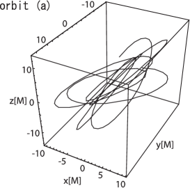
Figure 1: The orbit of a spinless particle with $E=0.968\mu,J_{z}=2.0\mu M,C=10\mu^{2}M^{2}$ and $a=1/\sqrt{2}$. We choose the initial position and velocity as $(r,\theta,\phi)=(10M,\pi/2,0)$ and $(v^{r},v^{\theta},v^{\phi})=(0.14,0.03,0.02)$. This is called the orbit (a) in this paper. This orbit looks very complicated as if chaos occurred.

This orbit is called the orbit (a) in this paper. The behavior of the orbit (a) looks complicated. However, showing the Poincaré map in Fig. 2, we find a closed curve, which confirms that the orbit (a) is not chaotic.

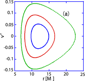
Figure 2: The Poincaré map of the orbit (a). The plot points form a closed curve in the two-dimensional $r$-$v^{r}$ plane. We also plot the Poincaré map of other two orbits with the same conserved quantities as those of the orbit (a). This confirms that the system is integrable.

III.1.2 a spinning particle

In the previous work Suzuki2 ; Suzuki3 , the parameter region for a spinning test particle in which a particle will show chaotic behavior was discussed. We adopt such parameters, e.g. the energy $E$, the angular momentum $J_{z}$, and the spin parameter $S$ of a test particle. Using the Bulirsch-Store method numerical , we integrate the equations of motion Eqs. (22)-(24) and use the constraint equations Eqs. (18),(26),(30),(31) to check the accuracy of our numerical integration. We find that the relative errors are smaller than $10^{-11}$ for each constraint. We show the orbits of the spinning particle in Fig. 3 and call it the orbit (b).

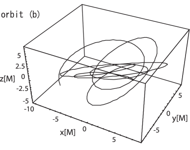
Figure 3: The orbits of a spinning particle with $E=0.9328\mu,J_{z}=2.8\mu M,$ and $S=1.0\mu M$. We set $a=0.8M$ and choose the initial position and velocity as $(r,\theta,\phi)=(6.0M,\pi/2,0)$ and $(v^{r},v^{\theta},v^{\phi})=(0.18,0.05,0.07)$. This is called the orbit (b), which is. complicated just as the orbit (a).

Comparing Fig. 1 with Fig. 3, we cannot distinguish two orbits. However, the difference between chaotic orbit and nonchaotic one will be apparent when we draw the Poincaré maps. In Fig. 4, we show the Poincaré map of the orbit (b).

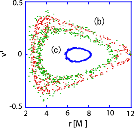
Figure 4: The Poincaré maps of the orbit (b) and (c). The plot points for the orbit (b) distribute randomly, which confirms that it is a chaotic system. For the orbit (c), we will discuss it later.

The plot points distribute randomly in Fig. 4. We also calculate the Lyapunov exponent $\lambda$ to evaluate the strength of chaos. The result is depicted in Fig. 5.

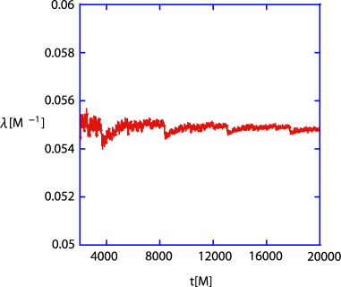
Figure 5: The maximal Lyapunov exponent $\lambda$ for the orbit (b). The typical time scale for chaos is given by $\lambda^{-1}\sim 18M$, while the average of orbital period is $74.3M$.

As shown in Fig. 5, the Lyapunov exponent $\lambda$ is positive, which means that the orbit (b) is chaotic. The typical time scale for chaos is given by $\lambda^{-1}\sim 18M$. Since the average of orbital period is $74.3M$, the orbit (b) becomes chaotic just after a few revolutions around a black hole.

III.2 Gravitational wave forms and energy spectra

Based on the previous calculation of the orbits, we show the wave forms and its energy spectra and analyze an effect of chaos on the emitted gravitational waves. To estimate the gravitational waves, we use the multipole expansion of gravitational field Mathews ; Kip . Here we briefly summarize the multipole expansion method. According to  Mathews ; Kip , the gravitational waves are represented in TT gauge as

$$h^{TT}_{ij}=\sum^{\infty}_{l=2}\sum^{l}_{m=-l}\frac{1}{r}\Big{(}\frac{d^{l}}{dt^{l}}I^{lm}(t-r)f_{ij}^{lm}+\frac{d^{l}}{dt^{l}}S^{lm}(t-r)d_{ij}^{lm}\Big{)},$$ (32)

where

$$f_{lm}=\frac{r^{2}}{\sqrt{4nl(l+1)}}\left(\begin{array}[]{ccc}0&0&0\\ 0&W_{lm}&X_{lm}\\ 0&*&-\sin^{2}\theta W_{lm}\end{array}\right),$$ (36)

$$d_{lm}=\frac{r^{2}}{\sqrt{4nl(l+1)}}\left(\begin{array}[]{ccc}0&0&0\\ 0&-X_{lm}/\sin\theta&\sin\theta W_{lm}\\ 0&*&\sin\theta X_{lm}\end{array}\right),$$ (40)

with

$$n=\frac{l(l+2)}{2}-1,$$ (41)

$$X_{lm}=2\frac{\partial}{\partial\phi}\Big{(}\frac{\partial}{\partial\theta}-\cot\theta\Big{)}Y_{lm},$$

$$W_{lm}=\Big{(}\frac{\partial^{2}}{\partial\theta^{2}}-\cot\theta\frac{\partial}{\partial\theta}-\frac{1}{\sin^{2}\theta}\frac{\partial^{2}}{\partial\phi^{2}}\Big{)}Y_{lm}\,.$$ (42)

($r$, $\theta$) is a position of an observer. $d_{lm}$ and $f_{lm}$ are an odd-parity and even-parity mode, respectively. $I^{lm}$ is a multipole of the mass distribution and $S^{lm}$ is that of the angular momentum. If a gravitational wave source moves slowly, we can write down $I^{lm}$ and $S^{lm}$ as

$$I^{lm} =\frac{16\pi}{(2l+1)!!}\Big{(}\frac{(l+1)(l+2)}{2(l-1)l}\Big{)}^{\frac{1}{2}}\int\tau_{00}Y^{*}_{lm}r^{l}d^{3}x,$$ (43)

$$S^{lm} =-\frac{32\pi}{(2l+1)!!}\Big{(}\frac{(l+2)(2l+1)}{2(l-1)(l+1)}\Big{)}^{\frac{1}{2}}$$

$$~{}~{}~{}\times\int\epsilon_{jpq}x_{p}(-\tau_{0q})Y^{l-1,lm*}_{j}r^{l-1}d^{3}x,$$ (44)

where $Y^{l-1,lm*}_{j}$ is called the pure orbital harmonic function

$$Y^{l^{\prime},lm}_{j}(\theta,\phi)=\sum^{l^{\prime}}_{m^{\prime}=-l^{\prime}}\sum^{1}_{m^{\prime\prime}=-1}(1l^{\prime}m^{\prime\prime}m^{\prime}|lm)\xi_{i}^{m^{\prime\prime}}Y^{l^{\prime}m^{\prime}},$$ (45)

$$\xi^{0}_{i}\equiv(\textbf{e}_{z})_{i},~{}~{}~{}\xi^{\pm}_{i}\equiv\mp\frac{1}{\sqrt{2}}(\textbf{e}_{x}\pm i\textbf{e}_{y})_{i}\,.$$ (46)

Giving the information of a particle orbit, we can evaluate $h_{ij}^{TT}$ for each $l$. The gravitational waves from a chaotic orbit of a spinning particle may contain higher multipole moments ($l>2$) than quadrupole ($l=2$). This is the reason why we analyze the gravitational waves not only $l=2$ but also $l=3$. Note that because the orbit considered here is very relativistic, the multipole expansion may not be valid and then it will provide only a qualitative feature.

In Fig. 6 and Fig. 7, we show the gravitational wave forms for the orbits (a) and (b), respectively.

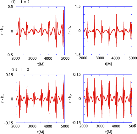
Figure 6: The gravitational wave forms of the $+$- and the $\times$-modes for the orbit (a). The observer is on the equatorial plane. Figs. (i) and (ii) show the wave forms of $l$= 2 and 3, respectively.

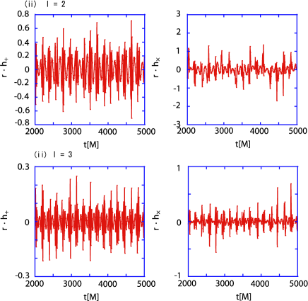
Figure 7: The gravitational wave forms of the $+$- and the $\times$-modes for the orbit (b). The observer is on the equatorial plane. Figs. (i) and (ii) show the wave forms of $l$= 2 and 3, respectively.

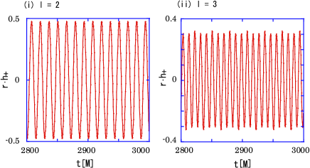
Figure 8: The wave forms for a circular orbit at $r=2.45M$.

These figures reveal two important points. One is that in the wave forms, there looks some difference between two orbits (a) and (b), but it may be difficult to distinguish which one is chaotic. Just as reference, we depict the wave form for a circular orbit in Fig. 8, which is quite regular. The second points is that the amplitudes of the octopole wave ($l=3$) are smaller than those of the quadrupole wave ($l=2$). Comparing the peak values, we find that the ratio of the amplitude of $l=3$ to that of $l=2$ is about 30 percents.

In Fig. 9, we show the energy spectrum of the quadrupole gravitational wave ($l=2$) from the orbit (a).

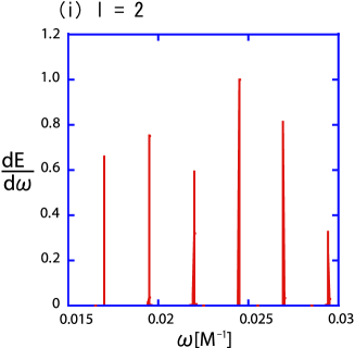
Figure 9: A energy spectrum of the gravitational wave from the orbit (a). Each value is normalized by the maximum peak value.

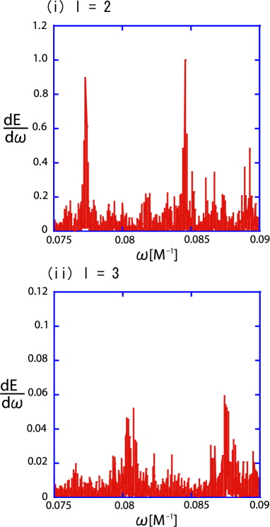
Figure 10: The energy spectra of the gravitational wave ($l=2,3$) from the spinning particle. (i)-(ii)The energy spectrum of the gravitational wave ($l=2,3$). The values in these case are normalized by the peak value of the spectrum $l=2$.

In Fig. 10, we show the energy spectrum of the gravitational wave($l=2,3$) from the spinning particle. From Fig. 9 and Fig. 10, we find that there is a clear difference in the energy spectra of the gravitational waves between the orbit (a) and (b).

How about the orbit of a spinning particle which looks regular? In order to understand a role of chaotic behavior, we also analyze the orbit (c), which Poincaré map is nearly a closed circle (the inner circle map in Fig. 4). Although this map looks closed in Fig. 4, we find that it is not really closed when we enlarge it (see Fig. 11).

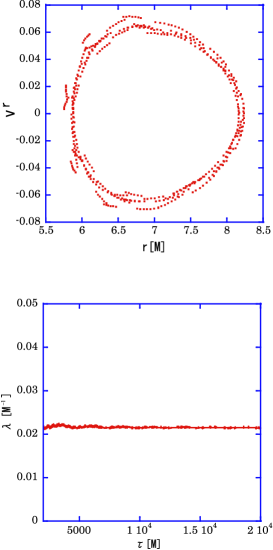
Figure 11: (i) The Poincaré map of the orbit (c). We also plot the Lyapunov exponent (ii), which value is smaller than that of the orbit (b) but is still positive ($\lambda\sim 0.02M$).

We show the wave forms for the orbit (c) in Fig. 12.

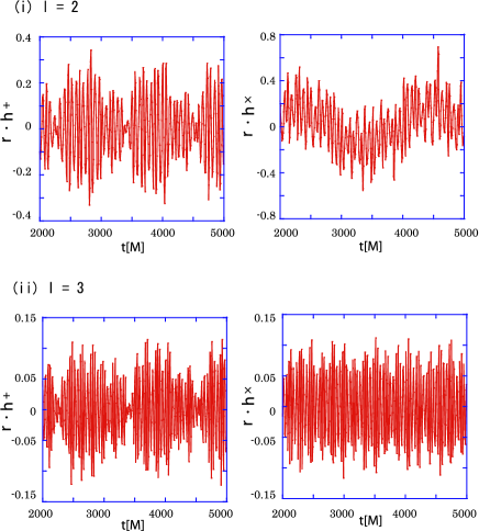
Figure 12: The gravitational wave forms of the $+$- and the $\times$-modes for the orbit (c). The observer is on the equatorial plane. Figs. (i) and (ii) show the wave forms of $l$= 2 and 3, respectively.

We also present the spectrum in Fig. 13.

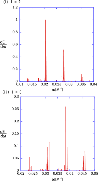
Figure 13: A energy spectrum of the gravitational wave from the orbit (c). This is similar to the orbit (a).

From the figures, we may conclude that the spectrum of gravitational waves from nonchaotic orbits contains only discrete characteristic frequencies. On the other hand, the spectrum for the chaotic orbits contains the various frequencies. It seems to be a continuous spectrum with finite widths. The ratio of the octopole wave energy for the orbit (b) to that of the quadrupole wave is about 12.4 percents. Therefore the higher pole moment than the quadrupole moment does not contribute so much to the emitted gravitational waves, although the orbit is chaotic.

IV Summary and Discussions

In this paper, we study the gravitational waves emitted from a chaotic dynamical system. As a concrete example, we analyze the motion of a test particle going around the Kerr black hole. We confirm that the orbit of a spinning particle can be chaotic. Using the multipole expansion method of a gravitational field, we evaluate the gravitational waves from a chaotic and a non-chaotic orbit in order to analyze the effect of chaos on the emitted gravitational waves. As the results, there are not so much difference for the gravitational wave forms. However, the energy spectra of the gravitational waves show a clear difference. For a chaotic orbit, we find a continuous energy spectrum with several peaks. While, in the case of nonchaotic orbit, the spectrum contains the discrete characteristic frequencies. We also find that the higher pole moments than quadrupole moment of the system do not contribute so much to the emitted gravitational waves even for a chaotic orbit.

When the gravitational waves are detected and the energy spectrum is determined by observation, not only the astrophysical parameters ,e.g., the mass, the angular momentum, and the spin are determined but also some fundamental physics such as relativistic nonlinear dynamics could be discussed.

As a future work, we have to study the gravitational waves in the dynamical system in a full relativistic approach. For the first step, using the Newmann-Penrose formalism NP , we extend the present evaluation (the multipole expansion) to a full relativistic perturbation analysis.

- (1) A. Abramovici, W. Althouse, R. Drever, Y. Gursel, S.Kawamura, F. Raab, D. Shoemaker, L. Sievers, R. Spero, K. Thorne, R. Vogt, R. Weiss, S. Whitcomb, and M. Zucker, Science 256,325(1992).
- (2) K. Tsubono, in proceedings of First Edoardo Amaldi Conference on Gravitational Wave Experiments, Villa Tuscolana, Frascati, Rome, edited by E. Coccia, G. Pizzella, and F. Ronga (World Scientific, Singapore. 1995), p112.
- (3) J. Hough, G. P. Newton, N. A. Robertson, H. Ward, A. M. Campbell, J. E. Logan, D. I. Robertson, K. A. Strain, K. Danzmann, H. Lück, A. Rüdiger, R. Schilling, M. Schrempel, W. Winkler, J. R. J. Bennett, V. Kose, M. Kühne, B. F. Scultz, D. Nicholson, J. Shuttleworth, H. Welling, P. Aufmuth, R. Rinkleff, A. Tünnermann, and B. Willke, in proceedings of the Seventh Marcel Grossman Meeting on recent developments in theoretical and experimental general relativity, gravitation and relativistic fiels theories, New Jersey, edited by R. T. Jantzen, G. M. Keiser, R. Ruffini, and R. Edge (World Scientific, 1996), p1352.
- (4) A. Giazotto, Nucl. instrum. Meth. A 289, 518(1990).
- (5) K. S. Thorne, in Prceedings of Snowmass 95 Summer Study on Particle and Nuclear Astrophysics and Cosmology, edited by E. W. Kolb and R. Peccei (World Scientific, Singapore. 1995), p398.
- (6) Deterministic Chaos in General Relativity, edited by D. Hobill, A. Burd, and A. Coley (Plenum, New York, 1994), and references therein.
- (7) J. D. Barrow, Phys. Rep. 85, 1 (1982).
- (8) G. Contopoulos, Proc. R. Soc. London A431,183(1990).
- (9) C. P. Dettmann, N. E. Frankel and N. J. Cornish, Phys. Rev. D 50, 618(1994).
- (10) U. Yurtsever, Phys. Rev. D 52,3176 (1995).
- (11) V. Karas and D. Vokrouhlický, Gen. Rela. Grav. 24,729(1992).
- (12) H. Varvoglis and D. Papadopoulos, Astron. Astrophys. 261,664(1992).
- (13) L. Bombelli and E. Calrzetta, Class. Quantum Grav. 9,2573(1992).
- (14) R. Moeckel, Commun. Math. Phys. 150,415(1992).
- (15) Y.Sota, S.Suzuki, and K. Maeda, Class. Quantum Grav. 13,1241(1996).
- (16) S. Suzuki and K. Maeda, Phys. Rev. D 55,4848(1997).
- (17) S. Suzuki and K. Maeda, Phys. Rev. D 58,023005(1998).
- (18) S. Suzuki and K. Maeda, Phys. Rev. D 61,024005(1999).
- (19) M. D. Hartl, Phys. Rev .D 67,024005(2003).
- (20) O. Semerák, Mon. Not. R. Astron. Soc 308,863(1999).
- (21) J. Levin, Phys. Rev. Lett. 84,3515(2000).
- (22) J. D. Schnittman and F. A. Rasio, Phys. Rev. Lett. 87, 121101 (2001).
- (23) N. J. Cornish and J. Levin, Phys. Rev. Lett. 89,179001(2002).
- (24) L. D. Landau and E. M. Lifshitz, The Classical Theory of Fields (Pergamon, Oxford, 1951).
- (25) J. Mathews, J. Soc. Ind. Appl. Math. 10,768(1962).
- (26) K. S. Thorne, Rev. Mod. Phys 52,299(1980).
- (27) B. Carter, Phys. Rev 174,1559(1968).
- (28) M. Johnston and R. Ruffini, Phys. Rev. D 10,2324(1974).
- (29) C. W. Misner, K. S. Thorne, and J. A. Wheeler, (W. H. Freeman and Company, New York, 1973).
- (30) A. Papapetrou, Proc. R. Soc. London A209,248(1951).
- (31) W. G. Dixon, Proc. R. Soc. London A314,499(1970); A319,509(1970).
- (32) W. Press, B. P. Flannery, S. Teukolosky and W. T. Vetterling, (Cambridge University Press, Cambridge, England, 1986).
- (33) E. T. Newman and R. Penrose, J. of Math. Phys. 3, 566(1962); 4, 998(1963).