Overview of the BlockNormal Event Trigger Generator

Abstract

In the search for unmodeled gravitational wave bursts, there are a variety of methods that have been proposed to generate candidate events from time series data. Block Normal is a method of identifying candidate events by searching for places in the data stream where the characteristic statistics of the data change. These change-points divide the data into blocks in which the characteristics of the block are stationary. Blocks in which these characteristics are inconsistent with the long term characteristic statistics are marked as Event-Triggers which can then be investigated by a more computationally demanding multi-detector analysis.

1 Finding Unmodeled Gravitational Waves

The ongoing search for the direct detection of gravitational waves using Earth based experiments involves the analysis of observations made at a variety of different detectors. These observations are time series samples of the detector state that are then processed by various means to identify gravitational wave candidates. Broadly speaking the searches for gravitational waves may be broken up into two categories, those searches that are based upon a model, such as the search for gravitational waves from inspiraling binaries, and those searches that endeavor to find gravitational waves without using a model. The latter category of searches are often referred to as “burst” searches. These searches typically seek to identify portions of data that are, for a short period, anomalously “loud” in comparison to the surrounding data.

Identifying a gravitational wave burst in the absence of a source model is an involved and potentially computationally expensive process. This is especially true when the ratio of signal power to noise power is low. A convenient and natural approach to mitigating the computational expense of identifying such bursts divides the problem of detection into two parts. In the first part, an inexpensive procedure is used to identify candidate sections of data that trigger the second part of the analysis. The second part of the analysis focuses on the subintervals of data identified by the first. It is a more computationally complex and expensive analysis that either discards the candidate or identifies it as a gravitational wave burst. In this way the first part of the analysis carried out by a so-called “event-trigger generator”, performs triage on the data that must be analyzed by the more complex second stage of the analysis.

2 The BlockNormal Pipeline

BlockNormal is an Event Trigger Generator that analyzes data in the time domain and searches for moments in time where the statistical character of the time series data changes. In particular, BlockNormal characterizes the time series between change-points by the mean($\mu$) and variance($\nu$) of the samples.

Change-points are thus demarcation points, separating “blocks” of data that are consistent with a distribution having a given mean and variance, which differs from the mean and/or variance that best characterizes the data in an adjacent block. The onset of a signal in the data will, because it is uncorrelated with the detector noise, increase the variance of the time series for as long as the signal is present with significant power. In this way blocks with variance greater than a “background” variance mark candidate gravitational wave bursts.

Since candidate gravitational wave bursts are identified with changes in the detector noise character it is best if the detector noise is itself stationary and white. The BlockNormal analysis thus starts by identifying long segments of data, epochs, which are relatively stationary. This process involves comparing adjacent stretches of data of fixed a duration long relative to the expected duration of a gravitational wave burst and asking whether adjacent stretches have consistent means and variances. In order to avoid any bias that might come from analyzing outliers in the tails of the distribution (where one might expect any true signal to be located), the mean and variance are computed on only those samples that are within the 2.5th and 97.5th percentiles of the sample values. If two consecutive stretches are inconsistent at the $95\%$ confidence level, the begining of the first stretch is used to define a new stationary segment.

Segments thus defined are split into a set of frequency bands whose lower band edge is heterodyned to zero frequency. This base-banding allows for a crude determination of the frequency of any identified triggers. Line and other spectral features are removed, either by Kalman filtering or by regression against diagnostic channels, and the final data whitened with a linear filter.

2.1 Finding Change-Points

Once the data has undergone the base-banding and whitening process, the search for change-points begins in earnest. The method employed is similar to that described in [1] and relies on a Bayesian analysis of the relative probability of two different hypotheses:

• $M_{1}$, that the time series segment $X_{N}$ is drawn from a distribution characterized by a single mean and variance; and

• $M_{2}$, that the time series segment $X_{N}$ consists of two continuous and adjacent subsegments each drawn from a distribution characterized by a different mean and/or variance.

Given the time series segment $X_{N}$, consisting of $N$ samples, we write the probability of hypothesis $M_{1}$ as $P(M_{1}|X_{N})$ and the probability of hypothesis $M_{2}$ as $P(M_{2}|X_{N})$. The odds of $M_{2}$ compared to $M_{1}$ is thus:

$$\rho_{2}=\frac{P(M_{2}|X_{N})}{P(M_{1}|X_{N})}$$ (1)

Applying Bayes Theorem and simplifying this becomes:

$$\rho_{2}=\frac{P(X_{N}|M_{2})}{P(X_{N}|M_{1})}\frac{P(M_{2})}{P(M_{1})}=\frac{P(X_{N}|M_{2})}{P(X_{N}|M_{1})}\gamma_{2}$$ (2)

where, $\gamma_{2}=\frac{P(M_{2})}{P(M_{1})}$ is independent of the data $X_{N}$ itself,although it does depend on the number of samples $N$.

If $M_{2}$ is true, then $M_{1}$ will be a good hypothesis for two subsets of the data, one from sample 1 to $j-1$, denoted $X_{1,j-1}$ and another from $j$ to $N$, $X_{j,N}$. Then we can write:

$$\rho_{2,j}=\gamma_{2}\frac{P(X_{j}|M_{1})P(X_{N-j}|M_{1})}{P(X_{N}|M_{1})}$$ (3)

$$\rho_{2}=\sum_{j=1}^{N-1}\rho_{2,j}$$ (4)

To calculate $\rho_{2}$ we thus need only be able to calculate $P(X_{N}|M_{1})$ for arbitrary time series $X_{N}$ The probability that a given data set is drawn from a normal distribution with unknown mean and variance is equal to:

$$P(X_{N}|M_{1})=\int d\sigma\int d\mu(2\pi\sigma^{2})^{-\frac{N}{2}}P(\mu,\sigma)\prod_{k=0}^{N-1}e^{-\frac{(x[k]-\mu)^{2}}{2\sigma^{2}}}$$ (5)

Where $P(\mu,\sigma)$ is the a priori probability that the mean takes on a value $\mu$ and the variance a value $\sigma^{2}$. With the usual uninformative priors for $\mu$ and $\sigma$ ($P(\mu)\propto\alpha$ and $P(\sigma)\propto\beta\sigma^{-1}$) the integral for $P(X_{N}|M_{1})$ can be evaluated in closed form:

$$P(X_{N}|M_{1})=\frac{\alpha\beta}{\sqrt{N}}[2\pi N(\overline{x^{2}}-\overline{x}^{2})]^{-\frac{(N-1)}{2}}I_{N-2}$$ (6)

$$I_{N}\equiv(N-1)!!\left\{\begin{array}[]{ll}1&\mbox{$N$ odd}\\ \sqrt{\frac{\pi}{2}}&\mbox{$N$ even}\end{array}\right.$$ (9)

where $\alpha\equiv P(\mu)$ an $\beta\equiv\sigma P(\sigma)$.

The value of $\rho_{2}$ is therefore the odds that there is a change-point in $X_{n}$ to there not being any change-points, and the value $\rho_{2,j}$ is related to the odds that there is a change-point at sample $j$ to there not being one anywhere in $X_{N}$. The calculated value of $\rho_{2}$ is compared to a threshold, $\rho_{T}$, and if greater than this threshold, a change-point is considered to be at the sample with the largest value of $\rho_{2,j}$.

Figure 1 shows some simulated data along with $\rho_{2,j}$ for that data. The two peaks in the value of $\rho_{2,j}$ corresponds to where the mean of the simulated noise changes.

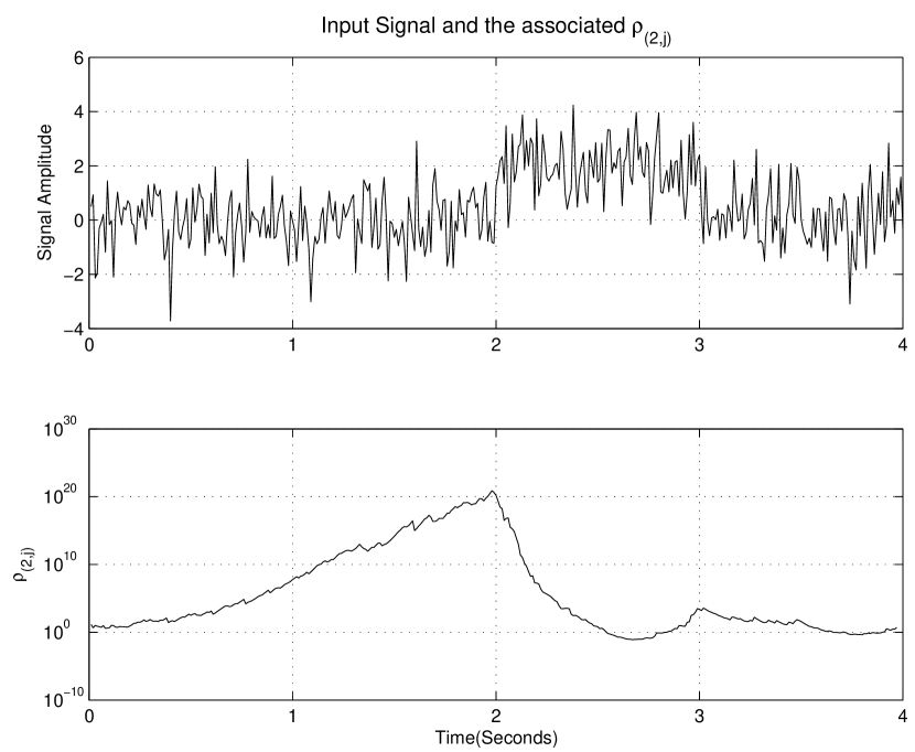
Figure 1: (top) A sample of simulated data consisting of blocks of white noise with a mean of two between two and three seconds and zero elsewhere. (bottom) The associated figure of merit, $\rho_{2,j}$ as a function of the hypothetical change point time.

This process either leaves $X_{N}$ free of change-points, or it divides the data into two subsets. In the latter case, the BlockNormal Pipeline repeats the change-point analysis on these subsets and all subsequent subsets, until either no more change-points are found, or the subset is less than 4 data points long. By this iteration method BlockNormal breaks the data at these change-points into a set of blocks, each of which is free of any change point. A final refinement step is taken where successive pairs of blocks are analyzed to check that the change-point would still be considered significant over the subset of the data that is contained within the two blocks.

2.2 Blocks, Events, and Clusters

BlockNormal identifies blocks — time series segments between successive change-points — are well characterized by a mean, a variance, a frequency band, a start time, and a duration. To identify unusual blocks, the means and variances are compared to the mean and variance, $\mu_{0}$ and $\sigma_{0}^{2}$ of all the data in their band from the epoch in which they were found. BlockNormal defines “Events” to be blocks in which the following condition holds true for a value, $C\equiv\max(\sigma^{2},(\mu-\mu_{0})^{2})$, that is used to characterize the block:

$$C>E_{T}\sigma_{0}^{2}$$ (10)

Here, $E_{T}$, is called the event threshold and is a free parameter in the algorithm which adjusts the sensitivity in defining what “unusual” means. There are a limited number of reasonable other possible threshold requirements based on the three characteristics of a block, $\mu$,$\sigma$,$D$, however, at this time these have not been explored.

Once events have been identified, immediately adjacent events in the same frequency band are clustered together, with a peak-time for the cluster defined by the central time of the block with the largest value of $C$. A cluster “Energy” is a sum over the $i$ blocks that comprise it:

$$\text{Energy}=\sum_{i}D_{i}\delta t\left[(\mu_{i}^{2}-\mu_{0}^{2})+\frac{D-1}{D}(\sigma_{i}^{2}-\sigma_{0}^{2})\right]$$ (11)

where $D_{i}$ is the duration in samples.

2.3 Defining Triggers

A key factor in building confidence in any identification of gravitational waves is the presence of a signal in different detectors. Using this “coincidence” as the basis for further reducing the number of periods of interest, BlockNormal requires that there be coincidence in time between events in the same band but different detectors before a “trigger” is formed. Triggers from different bands are merged if they overlap in time into a single trigger. Figure 2 illustrates how this coincidence and merging step works using the three LIGO interferometers.

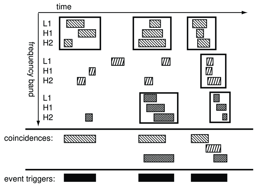
Figure 2: An illustration of how coincidence between different LIGO detectors and different frequency bands is used to create individual triggers.

3 Conclusion

The BlockNormal event trigger generator is a time domain analysis in base-banded data that identifies blocks in time which are well characterized by a mean and variance. blocks with means and variances that are unusually large compared to the mean and variance of the much longer data segment containing them are marked for consideration as being unusual events. Several coincident events in different detectors together form a trigger which can be used to define periods of interest that a more computationally intense analysis can use to reduce the total computing time needed to search for unmodeled gravitational wave events.

References

References

- [1] Smith A F M 1975 Biometrika 62,2 p. 407–416