Coincidence analysis to search for inspiraling compact binaries using TAMA300 and LISM data

Abstract

Japanese laser interferometric gravitational wave detectors, TAMA300 and LISM, performed a coincident observation during 2001. We perform a coincidence analysis to search for inspiraling compact binaries. The length of data used for the coincidence analysis is 275 hours when both TAMA300 and LISM detectors are operated simultaneously. TAMA300 and LISM data are analyzed by matched filtering, and candidates for gravitational wave events are obtained. If there is a true gravitational wave signal, it should appear in both data of detectors with consistent waveforms characterized by masses of stars, amplitude of the signal, the coalescence time and so on. We introduce a set of coincidence conditions of the parameters, and search for coincident events. This procedure reduces the number of fake events considerably, by a factor $\sim 10^{-4}$ compared with the number of fake events in single detector analysis. We find that the number of events after imposing the coincidence conditions is consistent with the number of accidental coincidences produced purely by noise. We thus find no evidence of gravitational wave signals. We obtain an upper limit of 0.046 /hours (CL $=90\%$) to the Galactic event rate within 1kpc from the Earth. The method used in this paper can be applied straightforwardly to the case of coincidence observations with more than two detectors with arbitrary arm directions.

I Introduction

In the past several years, there has been substantial progress in gravitational wave detection experiments by the ground-based laser interferometers, LIGOref:LIGOdescription , VIRGOref:virgo , GEO600ref:geo , and TAMA300ref:tama ; ref:ando . The observation of gravitational waves will not only be a powerful tool to test general relativity, but also be a new tool to investigate various unsolved astronomical problems and to find new objects which were not seen by other observational methods.

The Japanese two laser interferometers, TAMA300 and LISM, performed a coincident observation during August 1 and September 20, 2001 (JST). Both detectors showed sufficient stability that was acceptable for an analysis to search for gravitational wave signals. Given the sufficient amount of data, it was a very good opportunity to perform a coincidence analysis with real interferometers’ data.

There were several works to search for gravitational waves using interferometeric data. A coincidence analysis searching for generic gravitational wave bursts in a pair of laser interferometers has been reported in ref:Nicholson . Allen et al.ref:40m analyzed LIGO 40m data and obtained an upper limit of 0.5/hour (CL = 90$\%$) on the Galactic event rate of the coalescence of neutron star binaries with mass between 1$M_{\odot}$ and 3$M_{\odot}$. Tagoshi et al.ref:DT2 analyzed TAMA300 data taken during 1999 and obtained an upper limit of 0.59/hour (CL = 90$\%$) on the event rate of inspirals of compact binaries with mass between 0.3$M_{\odot}$ and 10$M_{\odot}$ and with signal-to-noise ratio greater than 7.2. Very recently, an analysis using the first scientific data of the three LIGO detectors was reported ref:LIGOinspiral , and an upper limit of $1.7\times 10^{2}$ per year per Milky Way Equivalent Galaxy is reported. Recently, International Gravitational Event Collaboration (IGEC) of bar detectors reported their analysis using four years of data to search for gravitational wave bursts ref:IGEC03 . They found that the event rate they obtained was consistent with the background of the detectors’ noise.

In the matched filtering analysis using real data of single laser interferometer (e.g. ref:40m , ref:DT2 ), many fake events were produced by non-Gaussian and non-stationary noise. In order to remove such fake events, it is useful to perform coincidence analysis between two or more independent detectors. Furthermore, coincidence analysis is indispensable to confirm the detection of gravitational waves when candidates for real gravitational wave signals are obtained. The purpose of this paper is to perform coincidence analysis using the real data of TAMA300 and LISM.

We consider gravitational waves from inspiraling compact binaries, comprized of neutron stars or black holes. They are consider to be one of the most promising sources for ground based laser interferometers. Since the waveforms of the inspiraling compact binaries are known accurately, we employ the matched filtering by using the theoretical waveforms as templates. Matched filtering is the optimal detection strategy in the case of stationary and Gaussian noise of detector. However, since the detectors’ noise is not stationary and Gaussian in the real laser interferomters, we introduce $\chi^{2}$ selection method to the matched filtering.

We analyze the data from each detector by matched filtering which produces event lists. Each event is characterized by the time of coalescence, masses of the two stars, and the amplitude of the signal. If there is a real gravitational wave event, there must be an event in each of the event list with consistent values of parameters. We define a set of coincidence conditions to search for coincident events in the two detectors. We find that we can reduce the number of events to about $10^{-4}$ times the original number. The coincidence conditions are tested by injecting the simulated inspiraling waves into the data and by checking the detection efficiency. We find that the detection efficiency is not affected significantly by imposing the coincidence conditions.

We estimate the number of coincident events produced accidentally by the instrumental noise. By using a technique of shifting the time series of data artificially, we find that the number of events survived after imposing the coincidence conditions is consistent with the number of accidental coincidences produced purely by noise.

We propose a method to set an upper limit to the real event rate using results of the coincidence analysis. In the case of TAMA300 and LISM, we obtain an upper limit of the event rate as 0.046/hour (CL = 90$\%$) for inspiraling compact binaries with mass between 1$M_{\odot}$ and 2$M_{\odot}$ which are located within 1kpc from the Earth. In this case, since TAMA300 is much more sensitive than LISM, the upper limit obtained from the coincidence analysis is less stringent than that obtained from the TAMA300 single detector data analysis. This is because the detection efficiency in the coincidence analysis is determined by the sensitivity of LISM. Thus, the upper limit obtained here is not the optimal one which we could obtain using the TAMA300 data taken during 2001.

The method to set an upper limit to the event rate proposed here can be extended straightforwardly to the case of a coincidence analysis for a network of interferometric gravitational wave detectors.

This paper is organized as follows. In Section II, we briefly describe the TAMA300 and LISM detectors. In Section III, we discuss a method of matched filtering search used for TAMA300 and LISM data. In Section IV, the results of the matched filtering search for each detector are shown. In section V, we discuss a method of the coincidence analysis using the results of single-detector searches, and the result of the coincidence analysis is shown. We also derive the upper limit to the event rate in Section VI. Section VII is devoted to summary. In Appendix A, we discuss a $\chi^{2}$ veto method to distinguish between real events and fake events produced by non-Gaussian noise. In Appendix B, we examine a different choice of $\Delta t$ ( the length of duration to find local maximum of matched filtering output ) for comparison. In Appendix C, we discuss a sidereal time distribution of coincidence events. In Appendix D, we review a method to estimate the errors in the parameters due to noise using the Fisher matrix.

Throughout this paper, the Fourier transform of a function $h(t)$ is denoted by $\tilde{h}(f)$, which is defined by

$$\tilde{h}(f)=\int_{-\infty}^{\infty}dt\ e^{2\pi ift}h(t).$$ (1)

II Detector

II.1 TAMA300

TAMA300 is a Fabry-Perot-Michelson interferometer with the baseline length of $300{\rm m}$ located at the National Astronomical Observatory of Japan in Mitaka, Tokyo ($35.68^{\circ}$N, $139.54^{\circ}$E) (See Table 1). The detector’s arm orientation (the direction of the bisector of two arms) measured counterclockwise from East is $225^{\circ}$. The details of TAMA300 detector configuration can be found in ref:ando . The TAMA300 detector became ready to operate in the summer 1999 ref:tama . Most of the designed system (except power recycling) were installed by the that time. First data taking was performed as a test during August 1999 (DT1). In September 1999, three days observation (DT2) was carried out, and the first search for gravitational waves from inspiraling compact binaries was performed ref:DT2 . Since then, TAMA300 has been performing several observations. In August 2000, an observation (DT4) was performed for two weeks and 160 hours of data were taken which are described in detail in ref:ando . From March 2nd to March 8th, 2001, TAMA300 performed an observation (DT5) and 111 hours of data were taken. After improvements of the sensitivity, TAMA300 had carried out a long observation (DT6) from August 1st to September 20th, 2001. The length of data taken was about 1100 hours. The best strain equivalent sensitivity was about $h\sim 5\times 10^{-21}/\sqrt{\rm Hz}$ around $800$Hz at DT6. From August 31th to September 2nd, 2002, TAMA300 performed a short observation (DT7) and 24 hours of data were taken. From February 14th and April 15th 2003, TAMA300 performed an observation (DT8) for two months, and 1158 hours of data were taken. Most recently, from November 28th 2003 to 10th January, 2004, TAMA300 performed an observation (DT9) and 557 hours of data were taken. The observation history of TAMA300 is summarized in Table 2.

In this paper, we use the DT6 data taken from September 2nd to 17th, 2001 when LISM was also in good condition. The amount of data available for the coincidence analysis is 275 hours in total. Typical one-sided noise power spectra of TAMA300 and LISM during this observation are shown in Fig. 1.

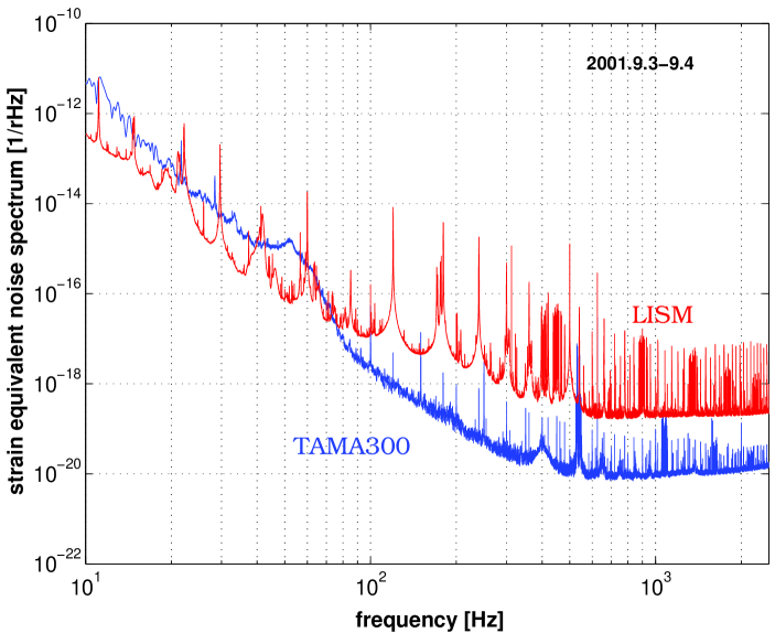
Figure 1: The strain equivalent noise spectra of TAMA300 and LISM on September 3, 2001.

	TAMA300 (DT6)	LISM
Interferometer type	Fabry-Perot-Michelson	Locked Fabry-Perot
Base length	300m	20m
Finesse of main cavity	500	25000
Laser Source	Nd:YAG, 10W	Nd:YAG, 700mW
Best sensitivity in strain $h\ {\rm[1/\sqrt{Hz}]}$	$5\times 10^{-21}$	$6.5\times 10^{-20}$
Location and arm orientation	$35.68^{\circ}$N, $139.54^{\circ}$E, $225^{\circ}$	$36.25^{\circ}$N, $137.18^{\circ}$E, $165^{\circ}$
Maximum delay of signal arrival time	$0.73$msec
Operation period	Aug.1 - Sept.20, 2001	Aug.1 - 23, Sept.3 - 17, 2001
Observation time	1038 hours	786 hours
Operation rate	87%	91%
Simultaneous observation	709 hours
Data used for coincidence analysis	275 hours

Table 1: Summary of the observation in August and September 2001 by TAMA300 and LISM

	Year	period	obsevation time [hours]	Topics
DT1	1999	6-7 Aug.	11	Total detector system check
				and Calibration test
DT2	1999	17-20 Sept.	31	First event search
DT3	2000	20-23 April	13	Sensitivity improved
DT4	2000	21 Aug.-4 Sept.	167	100 hours observation
DT5	2001	2-10 Mar.	111	Full time observation
DT6	2001	1 Aug.-20 Sept.	1038	1000 hours observation
				and coincident observation with LISM
DT7	2002	31 Aug.-2 Sept.	25	Power recycling installed (Full configuration)
DT8	2003	14 Feb.-14 April	1158	Coincident observation with LIGO
DT9	2003 - 2004	28 Nov.- 10 Jan.	557	Full automatic operation
				and Partial coincident observation
				with LIGO and GEO600

Table 2: Observation history of TAMA300

II.2 LISM

LISM is a laser interferometer gravitational wave antenna with arm length of 20m, located in the Kamioka mine ($36.25^{\circ}$N, $137.18^{\circ}$E), 219.02km west of Tokyo. The detector’s arm orientation is $165^{\circ}$ measured counter clockwise from East. The LISM antenna was originally developed as a prototype detector from 1991 to 1998 at the National Astronomical Observatory of Japan, in Mitaka, Tokyo, to demonstrate advanced technologies ref:sato . In 1999, it was moved to the Kamioka mine in order to perform long-term, stable observations. Details of the LISM detector is found in ref:satoLISM .

The laboratory site is 1000m underground in the Kamioka mine. The primary benefit of this location is extremely low seismic noise level except artificial seismic excitations. Furthermore, much smaller environmental variations at this underground site are beneficial to stable operation of a high-sensitivity laser interferometer. The optical configuration is the Locked Fabry-Perot interferometer. The finesse of each arm cavity was about 25000 to have a cavity pole frequency of 150Hz. The main interferometer was illuminated by a Nd:YAG laser yielding 700mW of output power, and the detector sensitivity spectrum was shot-noise limited at frequencies above about 1kHz.

The operation of LISM was started in early 2000, and has repeatedly been tested and improved since. The data used in this analysis were taken in the observations between August 1st and 23th and between September 3rd and 17th, 2001. The total length of data is 780 hours. The first half of the period was in a test-run and some improvements were made after that. The data from the second half were of good quality to be suitable for a gravitational wave event search, so 323 hours of data for the latter half was dedicated for this analysis. The best sensitivity during this period was about $h\sim 6.5\times 10^{-20}/\sqrt{\rm{Hz}}$ around 800Hz.

III Analysis method

III.1 Matched filtering

To search for gravitational waves emitted from inspiraling compact binaries, we use the matched filtering. In this method, cross-correlation between observed data and predicted waveforms are calculated to find signals and to estimate binary’s parameters. When the noise of a detector is Gaussian and stationary, the matched filtering is the optimal detection strategy in the sense that it gives the maximum detection probability for a given false alarm probability.

We use restricted post-Newtonian waveforms as templates: the phase evolution is calculated to 2.5 post-Newtonian order, and the amplitude evolution is calculated to the Newtonian quadrupole order. The effects of spin angular momentum are not taken into account here. The filters are constructed in Fourier domain by the stationary phase approximation ref:sfa of the post-Newtonian waveforms ref:pntemplate . We introduce the normalized templates ${h}_{c}$ and ${h}_{s}$ which are given in the frequency domain for $f>0$ by

$$\tilde{h}_{c}=Nf^{-7/6}\exp(i\Psi(f)),$$ (2)

$$\tilde{h}_{s}=iNf^{-7/6}\exp(i\Psi(f)),$$ (3)

where

$$\Psi(f) = 2\pi ft_{c}-{\pi\over 4}+{3\over 128\eta}(\pi GMfc^{-3})^{-5/3}\Bigg{[}1+\frac{1}{9}\left(\frac{3715}{84}+55\eta\right)(\pi GMfc^{-3})^{2/3}-16\pi(\pi Mfc^{-3})$$ (4)

$$+\left(\frac{15293365}{508032}+\frac{27145}{504}\eta+\frac{3085}{72}\eta^{2}\right)(\pi Mfc^{-3})^{4/3}+\frac{\pi}{3}\left(\frac{38645}{252}+5\eta\right)(\pi Mfc^{-3})^{5/3}\Bigg{]},$$

where $f$ is the frequency of gravitational waves, $t_{c}$ is the coalescence time, $M=m_{1}+m_{2}$, $\eta=m_{1}m_{2}/M^{2}$, and $m_{1}$ and $m_{2}$ are the masses of binary stars. For $f<0$, they are given by $\tilde{h}_{c/s}(f)=\tilde{h}_{c/s}^{*}(-f)$, where the asterisk denotes the complex conjugation. The normalization factor $N$ is defined such that $h_{c}$ and $h_{s}$ satisfy

$$({h}_{c},{h}_{c})=1,\quad\quad({h}_{s},{h}_{s})=1,$$ (5)

where

$$(a,b)\equiv 2\int^{\infty}_{-\infty}df{\tilde{a}(f)\tilde{b}^{*}(f)\over S_{n}(|f|)}.$$ (6)

$S_{n}(f)$ is the strain equivalent one-sided noise power spectrum density of a detector. We note that, for $\tilde{h}_{c}$ and $\tilde{h}_{s}$ calculated by the stationary phase approximation, we have $({h}_{c},{h}_{s})=0$.

In the matched filtering, we define the filtered output by

$$\tilde{\rho}=(s,{h}_{c}\cos(\phi_{c})+{h}_{s}\sin(\phi_{c})),$$ (7)

where $s(t)$ is the signal from a detector and $\phi_{c}$ is the phase of the template waveform. For a given interval of $t_{c}$, we maximize $\tilde{\rho}$ over the parameters $t_{c},$$M$, $\eta$ and $\phi_{c}$. The filtered output maximized over $\phi_{c}$ is given by

$$\tilde{\rho} = \sqrt{(s,{h}_{c})^{2}+(s,{h}_{s})^{2}}\equiv\rho.$$ (8)

The square of the filtered output, $\rho^{2}$, has an expectation value $2$ in the presence of only Gaussian noise in the data $s(t)$. Thus, we define the signal-to-noise ratio, SNR, by $\rho/\sqrt{2}$.

Matched filtering is the optimal detection strategy in the case of stationary and Gaussian noise of detector. However, since the detectors’ noise is not stationary and Gaussian in the case of real laser interferomters, we introduce $\chi^{2}$ method to the matched filtering in order to discriminate such noise from real gravitational wave signals. We describe details of $\chi^{2}$ method in Appendix A.

III.2 Algorithm of the matched filtering analysis

In this subsection, we describe a method to analyze time sequential data from the detectors by matched filtering.

First, we introduce, “a continuously locked segment”. The TAMA300 and LISM observations were sometimes interrupted by the failure of the detectors to function normally, which are usually called “unlock” of the detectors, or were interrupted manually in order to make adjustments to the instruments. A continuously locked segment is a period in which the detector is continuously operated without any interruptions and the data is taken with no dead time. In the analysis of this paper, we treat only the data in such locked segments.

The time sequential voltage data of a continuously locked segment are divided into small subsets of data with length of 52.4288 seconds (= sampling interval [s] $\times$ number of samples = $(5\times 10^{-5})\times 2^{20}$ [s]). Each subset of data has overlapping portions with adjacent subsets for 4.0 seconds in order not to lose signals which lie across borders of two adjacent subsets. The data of a subset are Fourier transformed into frequency domain and are multiplied by the transfer function to transform into strain equivalent data. The resulting subset of data is the signal of the detector in the frequency domain, $\tilde{s}(f)$, used in the matched filtering.

The power spectrum density of noise $S_{n}(f)$ is basically evaluated in a subset of data neighbouring to each $s(t)$ except for the cases below. On estimating the noise power spectrum, $S_{n}(f)$, we do not use the data contaminated by transient burst noise. For this purpose, we evaluate the fluctuation of the noise power defined by

$$p=\left[4\int_{0}^{\infty}{f^{-7/3}\over S_{n}(f)}df\right]^{-1/2},$$ (9)

for each set of data with length of 65.6 seconds which composes one file of stored data. We also calculate the average of $p$, $\langle p\rangle$, within each continuously locked segment. For each $\tilde{s}(f)$, we then apply the following criterion. If a subset of data in the neighborhood of $\tilde{s}(f)$ lies entirely in one of the files, we examine the value of $p$ of the file, and if it deviates from the average $\langle p\rangle$ for more than 2dB, i.e., $p>1.26\langle p\rangle$, we do not use that subset of data for evaluating the power spectrum and move to the neighboring subset. If a neighboring subset lies over two files, we examine the values of $p$ of the two files, and if either of them exceeds the 2dB level, we use neither of them. If a neiboring subset such that a file (or two consecutive files) that contains it has $p<1.26\langle p\rangle$ is found, the subset is divided into 8 pieces and the $S_{n}(f)$ is evaluated by taking the average of them. If the fluctuations of $p$ are too large, and we cannot find files with the values of $p$ within 2dB of the average within the locked segment, we use the power spectrum which is evaluated by taking the average of all the data in the corresponding locked segment.

In order to take the maximization of $\rho$ in Eq.(8) over the mass parameters, we introduce a grid in the mass parameter space. Each grid point defines the mass parameters which characterize a template. We adopt the algorithm introduced in ref:TT to define the grid point in the mass parameter space. The distance between the grid points is determined so as not to lose more than 3 $\%$ of signal-to-noise ratio due to mismatch between actual mass parameters and those at grid points. Accordingly, the mass parameter space depends on the power spectrum of noise. In order to take into account of the changes in the noise power spectrum with time, we use different mass parameter spaces for different locked segments. For each locked segment, the averaged power spectrum of noise is used to determine the grid spacing in the mass parameter space.

We consider the mass of each component star in the range $1M_{\odot}\leq m_{1},\,m_{2}\leq 2M_{\odot}$. This mass range is chosen so that it covers the most probable mass of a neutron star, $\sim 1.4M_{\odot}$.

With $\tilde{s}(f)$, $S_{n}(f)$ and a template on each grid point of the mass parameter space, we calculate $\rho$ in Eq. (8). For each interval $\Delta t=25.6$ msec, we search for $t_{c}$ at which the local maximum of $\rho$ is realized. If the $\rho$ thus obtained is greater than a pre-determined value $\rho_{m}$, we calculate the value of $\chi^{2}$ as discussed in Appendix A. We adopt $\rho_{m}=7$ in this paper. Choosing a too large $\rho_{m}$ results in missing actual events from the data, while a too small $\rho_{m}$ requires too much computational time. The same computation is done for all the mass parameters on each grid point.

Finally, for each interval of the coalescence time with length $\Delta t=25.6$ msec, we search for $t_{c}$, $M$, $\eta$ which realize the local maximum of $\rho$. Each maximum is considered a event. The value of $t_{c}$, $\rho$, $\chi^{2}$, $M$, $\eta$ of each event are recorded in event lists.

IV Results of matched filtering search

In this section, we show the result of the independent analysis for each detector.

Our analysis is carried out with 9 Alpha computers and also with 12 Pentium4 computers at Osaka University. The matched filtering codes are paralleled by the MPI library. Among the data from September 3rd to 17th, 2001, TAMA300 has 292.4 hours of data after removing unlocked periods. We also removed the data segments of lengths less than 10 minutes. The total length of data is 287.6 hours. LISM has 323.0 hours of data after removing unlocked periods. After removing the data segments less than 10 minutes, the total length of data is 322.6 hours.

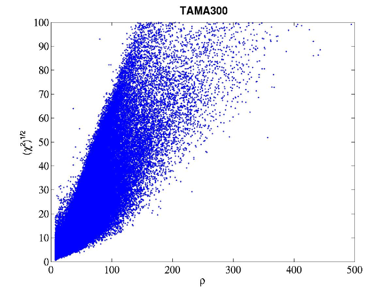
Figure 2: Scatter plots ($\rho,\sqrt{\chi^{2}}$) of the events of TAMA300.

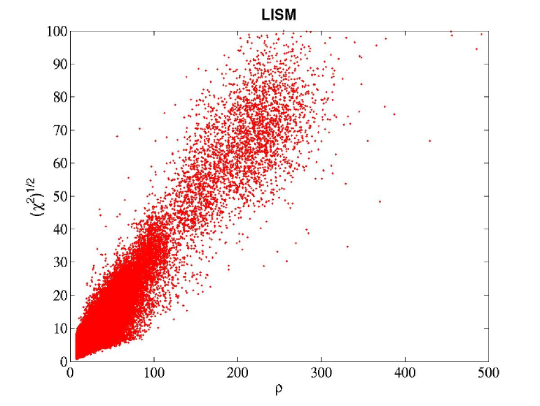
Figure 3: The same figure as Fig.2 but for LISM.

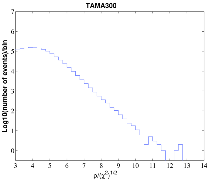
Figure 4: Histogram of the number of events of TAMA300 in terms of $\rho/\sqrt{\chi^{2}}$.

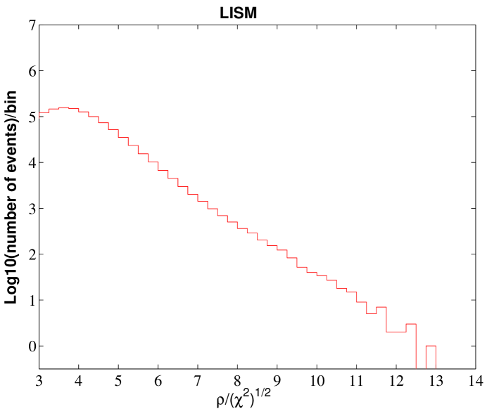
Figure 5: The same figure as Fig.4 but for LISM.

The scatter plots of $(\rho,\sqrt{\chi^{2}})$ of the events are shown in Figs. 2 and 3. We discriminate the non-Gaussian noise from real gravitational wave signals by setting the threshold to the value of $\rho/\sqrt{\chi^{2}}$ (see Appendix A). In Figs. 4 and 5 , we show the number of events for bins of $\rho/\sqrt{\chi^{2}}$.

Although the main topic of this paper is to perform a coincidence analysis, for the purpose of comparison between a single-detector analysis and a coincidence analysis, we evaluate the upper limit to the event rate which is derived from an analysis independently done for each detector. The upper limit to the Galactic event rate is calculated by ref:40m

$$R=\frac{N}{T\epsilon}$$ (10)

where $N$ is the upper limit to the average number of events with $\rho/\sqrt{\chi^{2}}$ greater than a pre-determined threshold, $T$ is the total length of data [hours] and $\epsilon$ is the detection probability.

To examine the detection probability of the Galactic neutron star binary events, we use a model of the distribution of neutron star binaries in our Galaxy which is given by ref:neutronstar

$$dN=e^{-R^{2}/2R_{0}^{2}}e^{-Z/h_{z}}RdRdZ,$$ (11)

where $R$ is Galactic radius, $R_{0}=4.8$ kpc, $Z$ is height off the Galactic plane and $h_{z}=1$ kpc is the scale height. We assume that the mass distribution is uniform between $1M_{\odot}$ and $2M_{\odot}$. We also assume uniform distributions for the inclination angle and the phase of an event. With these distribution functions, we perform a Monte Carlo simulation. The simulated gravitational wave events are injected into the data of each detector for about every 15 minutes. We perform a search using the same code used in our matched filter analysis, and evaluate the detection probability for each $\rho/\sqrt{\chi^{2}}$ threshold. The result for TAMA300 is shown in Fig. 6.

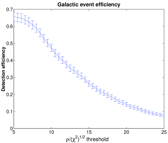
Figure 6: Galactic event detection efficiency of TAMA300. The error bars shows the $1\sigma$ error of the simulation.

For the case of LISM, since LISM’s sensitivity is not good enough to observe events in all of the Galaxy, we only evaluate the detection probability of nearby events within 1kpc. The result is shown in Fig. 7.

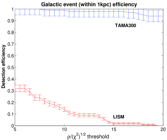
Figure 7: The detection efficiency of TAMA300 and LISM for nearby events within 1kpc. The error bars show the $1\sigma$ error of the simulation.

The threshold of $\rho/\sqrt{\chi^{2}}$ for each of the analysis is determined by the fake event rate. We set the fake event rate to be $2.0$ [1/yr]. We approximate the distribution of $\rho/\sqrt{\chi^{2}}$ in each of Figs. 4 and 5 by an exponential function and extrapolate it to large $\rho/\sqrt{\chi^{2}}$. We assume that this function describes the background fake event distribution.

For the TAMA300 case, the fake event rate $N_{\rm bg}/T=2.0$ [1/yr] $=0.00023$ [1/hour] gives the total number of expected fake events as $N_{\rm bg}=0.066$. This determines the threshold to be $\rho/\sqrt{\chi^{2}}=14.8$. With this threshold, we obtain the detection probability, $\epsilon=0.263$, from Fig. 6. On the other hand, the number of observed events with $\rho/\sqrt{\chi^{2}}$ greater than the threshold is $N_{\rm obs}=0$. Using Bayesian statistics, and assuming uniform prior probability for the real event rate and the Poisson distributions for real and background events, we estimate the expected number of real events $N$ which $\rho/\sqrt{\chi^{2}}$ is greater than the threshold with a given confidence level (CL). Namely, it can be evaluated from the equation ref:basian ,

$${{e^{-(N+N_{\rm bg})}\sum_{n=0}^{n=N_{\rm obs}}{(N+N_{\rm bg})^{n}\over n!}}\over{e^{-N_{\rm bg}}\sum_{n=0}^{n=N_{\rm obs}}{(N_{\rm bg})^{n}\over n!}}}=1-\rm{CL}\,.$$ (12)

Using this formula, we obtain the upper limit to the expected number of real events to be 2.30 with $90\%\,\rm{CL}$. Then, using the length of data $T=287.6$ hours, we obtain the upper limit of the event rate as $R_{90\%}=0.030$ [1/hour] ($\rm{CL}=90\%$).

For the LISM detector, we only evaluate the upper limit to nearby events within 1kpc. We set the threshold $\rho/\sqrt{\chi^{2}}=14.6$, corresponding to the number of expected fake events $N_{\rm bg}=0.074$ which realizes the fake event rate $N_{\rm bg}/T=2.0$ [1/yr]. The number of observed events with $\rho/\sqrt{\chi^{2}}$ greater than the threshold is $N_{\rm obs}=0$. Thus, the upper limit to the expected number of real events is again $2.30$ with $90\%$ CL. The detection probability is given from Fig.7 as $\epsilon=0.042$. The length of data is $T=322.6$ hours. Using these numbers, we obtain the upper limit to the nearby event rate as $0.17$ [1/hour] with $90\%\,\rm{CL}$.

The results of matched filtering analysis for TAMA300 and LISM are summarized in Table 3.

	threshold	N	Detection efficiency	Length of data	Upper limit (90% CL)
TAMA300	14.8	2.30 (90% CL)	0.263	287.6 [hours]	0.030 [1/hour]
LISM	14.6	2.30 (90% CL)	0.042	322.6 [hours]	0.17 [1/hour] (for nearby events)

Table 3: Results of matched filtering analysis for TAMA300 and LISM

V Coincidence analysis

V.1 Method

In the previous section, we obtained event lists for TAMA300 and LISM. Each event is characterized by $t_{c}$, ${\cal M}$, $\eta$, $\rho$, and $\chi^{2}$, where ${\cal M}$ is the chirp mass ($=M\eta^{3/5}$). True gravitational wave events will appear in both event lists with different values of these parameters according to the detectors’ noise, the difference in the detectors’ locations and thier arm orientations, and the discreteness of the template space. In this section, we evaluate the difference of the parameters real events have.

Time selection:

The distance between the TAMA300 site and the LISM site is 219.02km. Therefore, the maximum delay of the arrival time of gravitational wave signals is $\Delta t_{\rm dist}=0.73057$ msec. The allowed difference in $t_{c}$ is set as follows. If the parameter, $t_{c,{\mbox{\rm\tiny TAMA}}}$ and $t_{c,{\mbox{\rm\tiny LISM}}}$, of an event satisfy

$$|t_{c,{\mbox{\rm\tiny TAMA}}}-t_{c,{\mbox{\rm\tiny LISM}}}|<\Delta t_{\rm dist}+\Delta t_{\rm noise},$$ (13)

the event is recorded in the list as a candidate for real events. We estimate errors in $t_{c}$ due to noise $\Delta t_{\rm noise}$ by using the Fisher information matrix (see Appendix D for a detailed discussion). We denote the 1 $\sigma$ value of the error of $t_{c}$ by $\Delta t_{c,i}$ for $i=$ TAMA or LISM. We determine $\Delta t_{\rm noise}$ as $\Delta t_{{\rm noise}}=\sigma_{w}\times\Delta t_{c}$ where $\Delta t_{c}=\sqrt{\Delta t^{2}_{c,{\mbox{\rm\tiny TAMA}}}+\Delta t^{2}_{c,{\mbox{\rm\tiny LISM}}}}$. The parameter $\sigma_{w}$ is to be determined in such a way that it is small enough to exclude accidental coincidence events effectively but is large enough to make the probability for missing a real event sufficiently small.

In this paper, we adopt $\sigma_{w}=3.29$ which corresponds to 0.1$\%$ probability of losing real signals if the noise are Gaussian and if both detectors are located at the same site. Although it may be possible to tune the value of $\sigma_{w}$ to obtain a better detection efficiency while keeping the fake event rate low enough, we do not bother to do so. Instead, we check whether we have a reasonable detection efficiency by this choice. To check the detection efficiency is important in any case, since the $\Delta t_{c}$ determined above assumes a large signal amplitude in the presence of Gaussian noise. The actual detection efficiency might be different from what we expected.

Mass selection:

In the same way as for $t_{c}$, errors in the values of $\mathcal{M}$ and $\eta$ due to detector noise, $\Delta\mathcal{M}_{\rm noise}$ and $\Delta\eta_{\rm noise}$, are estimated by using the Fisher matrix. We denote the 1 $\sigma$ values of errors in $\mathcal{M}$ and $\eta$ by $\Delta\mathcal{M}_{i}$ and $\Delta\mathcal{\eta}_{i}$, respectively. We set $\Delta\mathcal{M}_{\rm noise}=\sigma_{w}\sqrt{(\Delta\mathcal{M})^{2}_{\mbox{\rm\tiny TAMA}}+(\Delta\mathcal{M})^{2}_{\mbox{\rm\tiny LISM}}}$ and $\Delta\eta_{\rm noise}=\sigma_{w}\sqrt{(\Delta\eta)^{2}_{\mbox{\rm\tiny TAMA}}+(\Delta\eta)^{2}_{\mbox{\rm\tiny LISM}}}$, and adopt $\sigma_{w}=3.29$ as in the case of $t_{c}$.

When the amplitude of a signal is very large, errors due to detector noise become small since they are inversely proportional to $\rho$, and errors due to the discreteness of the mass parameter space become dominant. We denote the latter errors by $\Delta\mathcal{M}_{\rm mesh}$ and $\Delta\eta_{\rm mesh}$. They are determined from the maximum difference in the neighbouring mesh points in the mass parameter space.

By taking account of the above two effects, we choose the allowable difference in the mass parameters as

$$|\mathcal{M}_{\rm TAMA}-\mathcal{M}_{\rm LISM}| < \Delta\mathcal{M}_{\rm noise}+\Delta\mathcal{M}_{\rm mesh},$$ (14)

$$|\eta_{\rm TAMA}-\eta_{\rm LISM}| < \Delta\eta_{\rm noise}+\Delta\eta_{\rm mesh}.$$ (15)

Amplitude selection:

Since the two detectors have different sensitivities, signal-to-noise ratios of an observed gravitational wave signal will be different for the two detectors. Further, since their arm orientations are different, the signal-to-noise ratios will differ even if they have the same noise power spectrum.

We express the allowable difference in $\rho_{\mbox{\rm\tiny TAMA}}$ and $\rho_{\mbox{\rm\tiny LISM}}$ as

$$\delta_{\rm sens}-\delta_{\rm arm}-\delta_{\rm noise}\leq\log\Big{(}{\frac{\rho_{\mbox{\rm\tiny TAMA}}}{\rho_{\mbox{\rm\tiny LISM}}}}\Big{)}\leq\delta_{\rm sens}+\delta_{\rm arm}+\delta_{\rm noise}.$$ (16)

Here, $\delta_{\rm sens}$ is due to the difference in $S_{n}$,

$$\delta_{\rm sens}\equiv\log\Big{[}\Big{(}\int\frac{f^{-7/3}}{S_{n\ {\mbox{\rm\tiny TAMA}}}(f)}df\Big{)}^{1/2}/\Big{(}\int\frac{f^{-7/3}}{S_{n\ \mbox{\rm\tiny LISM}}(f)}df\Big{)}^{1/2}\Big{]},$$ (17)

and $\delta_{\rm arm}$ is due to the difference in the arm orientations, and $\delta_{\rm noise}$ is due to detector noise. The value of $\delta_{\rm noise}$ is evaluated by the Fisher matrix in the same way as $t_{c}$ and masses.

The value of $\delta_{\rm sens}$ is determined for each event individually from the noise power spectrum used in the matched filtering. $\delta_{\rm arm}$ is evaluated by a Monte Carlo simulation as follows. We assume that the two detectors have the same noise power spectrum, and generate the waveforms of Galactic events randomly. We then evaluate $\rho$ of all the events detected by each detector, and determine the value of $\delta_{\rm arm}$ in such a way that for more than 99.9 % of events, we have $|\log(\rho_{\mbox{\tiny TAMA}}/\rho_{\mbox{\tiny LISM}})|\leq\delta_{\rm arm}$. This gives $\delta_{\rm arm}=1.60$.

V.2 Detection efficiency and the parameter windows

Here, we discuss the detection efficiency of our coincidence analysis. In particular, we examine the validity of the choice $\sigma_{w}=3.29$ made in the previous section.

For the Galactic event simulation discussed in Section IV, the detection efficiencies of TAMA300 and LISM for the threshold $\rho/\sqrt{\chi^{2}}>7$ are 99% and 24%, respectively. The detection efficiency of the coincidence analysis is dominated by the LISM’s efficiency. Thus we define the detection efficiency for the coincidence analysis, as the fraction of LISM events which fulfill the coincidence criteria. The result is shown in Fig. 8. We find that more than 94 % of LISM events can be detected if we set $\sigma_{w}>3$. Thus with $\sigma_{w}=3.29$, we have a reasonably high detection efficiency.

If we adopt a larger value of $\sigma_{w}$, we obtain a higher detection efficiency, but the number of fake events will also increase, and vise versa for a smaller value of $\sigma_{w}$. Then, one may tune the value of $\sigma_{w}$ so that it gives the most stringent upper limit to the event rate. However, since we cannot expect any drastic improvement by such an optimization, we adopt $\sigma_{w}=3.29$ in this paper for the sake of simplicity of the analysis.

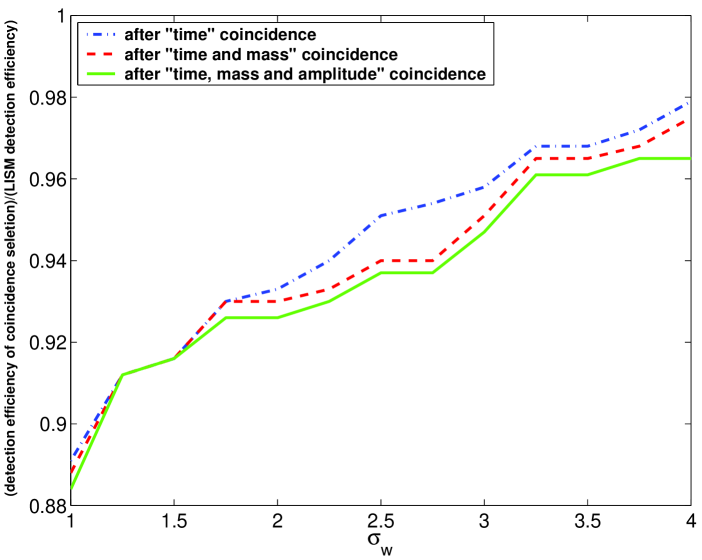
Figure 8: Relative detection efficiency of the coincidence analysis compared to the single-detector efficiency of LISM as a function of the parameter $\sigma_{w}$ used for the coincidence criterion. The dot-dashed line is the efficiency after the time selection, the dashed line is the efficiency after the time and mass selection, and the solid line is the efficiency after the time-mass-amplitude selection.

V.3 Results

In this subsection we discuss the results of the coincidence analysis. The length of data used for the coincidence analysis is 275.3 hours when both TAMA300 and LISM detector were operated simultaneously.

As a result of independent matched filtering searches, we obtained 1,868,388 events from the TAMA300 data and 1,292,630 events from the LISM data. For these events, we perform the time, mass and amplitude selections discussed in the previous section. In Fig. 9, we show a scatter plot of the events after coincidence selections in terms of $\rho_{\mbox{\rm\tiny TAMA}}$ and $\rho_{\mbox{\rm\tiny LISM}}$. A significant number of events are removed by imposing coincidence conditions. Only $0.04\%$ of the TAMA300 events remain. In Table 4, we show the number of events which survived after the selections.

We reduce the fake events by introducing the renormalization $\rho$ by $\chi^{2}$ in addition to the coincidence conditions. In Fig. 10, we show a scatter plot of these events in terms of the value of $\rho_{\mbox{\rm\tiny TAMA}}/\sqrt{\chi^{2}_{\mbox{\rm\tiny TAMA}}}$ and $\rho_{\mbox{\rm\tiny LISM}}/\sqrt{\chi^{2}_{\mbox{\rm\tiny LISM}}}$.

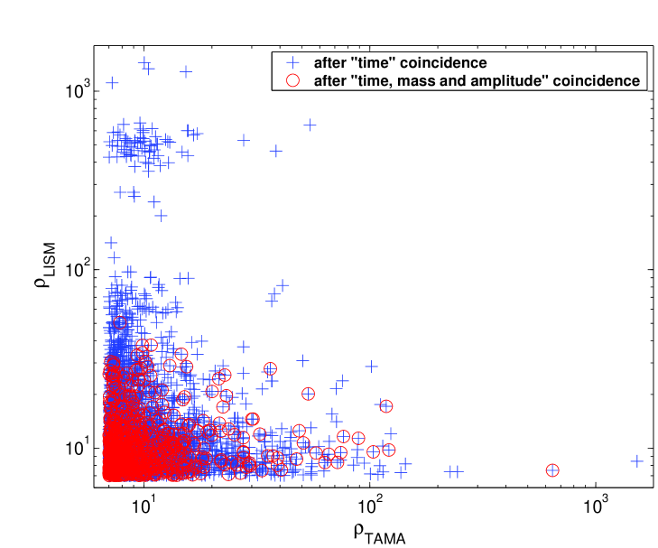
Figure 9: ($\rho_{\mbox{\rm\tiny TAMA}}$ ,$\rho_{\mbox{\rm\tiny LISM}}$) scatter plots.The crosses (+) are the events survived after the time selection, and the circled crosses ($\oplus$) are the events survived after the time, mass and amplitude selections.

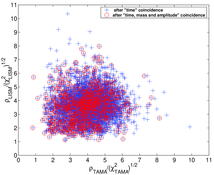
Figure 10: ($\rho_{\mbox{\rm\tiny TAMA}}/\sqrt{\chi^{2}_{\mbox{\rm\tiny TAMA}}}$ ,$\rho_{\mbox{\rm\tiny LISM}}/\sqrt{\chi^{2}_{\mbox{\rm\tiny LISM}}}$) scatter plots.The crosses (+) are the events survived after the time selection, and the circled crosses ($\oplus$) are the events survived after the time, mass and amplitude selections.

Results of independent matched filtering searches
	TAMA300	LISM
Number of events	1,868,388	1,292,630
Results of coincidence analysis
	$n_{\rm obs}$	$\bar{n}_{\rm acc}\pm\bar{\sigma}_{\rm acc}$
after time selection	4706	$(4.2\pm 0.5)\times 10^{3}$
after time and mass selection	804	$(7.1\pm 0.8)\times 10^{2}$
after time, mass and amplitude selection	761	$(6.7\pm 0.8)\times 10^{2}$
Threshold	$N_{\rm obs}$	$N_{\rm bg}$
$\rho_{\mbox{\rm\tiny TAMA}}/\sqrt{\chi^{2}_{\mbox{\rm\tiny TAMA}}}>8.3$ and $\rho_{\mbox{\rm\tiny LISM}}/\sqrt{\chi^{2}_{\mbox{\rm\tiny LISM}}}>8.1$	0	0.063

Table 4: Results of coincidence analysis. $n_{\rm obs}$ is the number of coincidence events. $\bar{n}_{\rm acc}$ and $\bar{\sigma}_{\rm acc}$ are the estimated number of accidental coincidence and its variance, respectively. Note that the mean number of accidentals and their variance after the time selection procedure affect those after the time and mass selection procedure, and the latter affect those after the time, mass and amplitude selection procedure. Thus, because the observed number of coincidence events is consistent with the expected number of accidental coincidence after the time selection procedure, it is not unnatural to find a good agreement between the observed value and the expectation value in each of the subsequent selection procedures.

In order to obtain statistical significance from the above results, the number of coincident events should be compared with the number of accidental coincidences produced purely by noise events. If events occur completely randomly, and its event rate in each detector is stationary, the average number of accidental coincidences after the time selection is given by

$$\bar{n}_{\rm pr}=N_{\mbox{\rm\tiny TAMA}}N_{\mbox{\rm\tiny LISM}}\frac{\Delta\bar{t_{c}}^{\rm window}}{T_{\rm obs}},$$ (18)

where $N_{\mbox{\rm\tiny TAMA}}$ and $N_{\mbox{\rm\tiny LISM}}$ are the number of events in each detector, $T_{\rm obs}$ is the total observation time, and $\Delta\bar{t}_{c}^{\rm window}$ is the averaged value of the time selection window. The averaged value of the time selection window is evaluated as $\Delta\bar{t}_{c}^{\rm window}=1.29$ msec. We thus obtain $\bar{n}_{\rm pr}=6.3\times 10^{3}$, which is slightly larger than the observed number of coincidence, 4706, after the time selection. One reason for this diffrence is that the event trigger rate is not stationary over the whole period of this observation.

In order to obtain a more reliable value for the rate of accidental coincidence, we use the time shift procedure. Namely, we shift all events of one detector by a time $\delta t$ artificially (which is called the time delay), and perform coincidence searches to determine the number of accidental events $n_{c}(\delta t)$ for various values of $\delta t$ ref:Amaldi ref:Astone . With $m$ different values of time delay, we calculate the expected number of coincident events and its standard deviation as

$$\bar{n}_{\rm acc}=\frac{1}{m}\sum_{i=1}^{m}n_{c}(\delta t_{i}),$$ (19)

$$\bar{\sigma}_{\rm acc}=\sqrt{\sum_{i=1}^{m}\Big{(}n_{c}(\delta t_{i})-\bar{n}_{\rm acc}\Big{)}^{2}/(m-1)}.$$ (20)

Since there is no real coincidence if $|\delta t|\gg\Delta t_{\rm dis}$, the distribution of the number of coincidences with time delay can be considered as an estimation of the distribution of accidental coincidences. The number of coincident events, $n_{c}(0)$, is compared to the estimated distribution.

Fig. 11 shows the time delay histograms with $m=400$. The 400 time delays are chosen from $-12000$ sec to $12000$ sec in increments of 60 seconds. The distribution of accidentals is shown in Fig. 12. In Table 4, we also list the expectation values of the number of accidental coincidence and the standard deviation after each selection procedure. As can be seen from this, the number of coincident events after each selection procedures is consistent with the expected number of accidental coincidences within the statistical fluctuations. Thus, we conclude that no statistically significant signals of real coincident events are observed in our search.

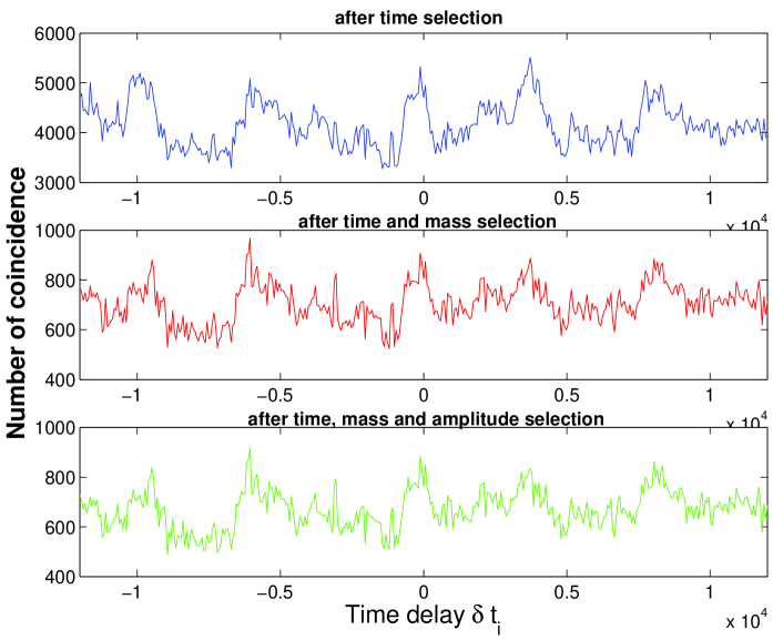
Figure 11: From top to bottom, the time delay histogram after time selection, after time and mass selection, and after time, mass and amplitude selection, respectively, are plotted.

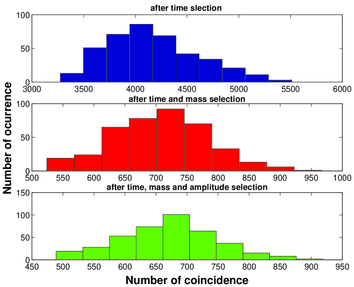
Figure 12: The distribution of the number of realizations with 400 different time delays with respect to the number of coincidences derived from Fig. 11. From top to bottom, the distribution after time selection, after time and mass selection, and and after time, mass and amplitude selection are plotted.

VI Upper limit to the event rate from coincidence analysis

In this section, we present a method to evaluate the upper limit to the event rate based on the above result of the coincidence analysis.

The upper limit to the event rate is given by Eq. (10) as in the case of the single-detector searches. The upper limit $N$ to the average number of real events can be determined by Eq. (12), using the observed number of events $N_{\rm obs}$ with $\rho/\sqrt{\chi^{2}}$ greater than the threshold, the estimated number of fake events $N_{\rm bg}$ with $\rho/\sqrt{\chi^{2}}$ greater than the threshold, and the confidence level. We set different thresholds to the value of $\rho_{\mbox{\rm\tiny TAMA}}/\sqrt{\chi_{\mbox{\rm\tiny TAMA}}^{2}}$ and $\rho_{\mbox{\rm\tiny LISM}}/\sqrt{\chi_{\mbox{\rm\tiny LISM}}^{2}}$ respectively. An advantage of this is that, because of its simplicity, it can be readily applied to the cases when more than two detectors with different arm directions are involved.

We determine a background distribution $f(y_{1},y_{2})$ of the number of coincident events from the data for $y_{1}>5.5$ or $y_{2}>5.5$ in Fig. 10, where $y_{1}=\rho_{\mbox{\rm\tiny TAMA}}/\sqrt{\chi_{\mbox{\rm\tiny TAMA}}^{2}}$ and $y_{2}=\rho_{\mbox{\rm\tiny LISM}}/\sqrt{\chi_{\mbox{\rm\tiny LISM}}^{2}}$. We evaluate the expected number of fake events which $\rho/\sqrt{\chi^{2}}$ is greater than the thresholds $y_{1}=y_{\mbox{\rm\tiny T}}$ or $y_{2}=y_{\mbox{\rm\tiny L}}$ by

$$N_{bg}=\int_{y_{\rm\scriptscriptstyle T}}^{\infty}dy_{1}\int_{0}^{\infty}dy_{2}f(y_{1},y_{2})+\int_{0}^{\infty}dy_{1}\int_{y_{\rm\scriptscriptstyle L}}^{\infty}dy_{2}f(y_{1},y_{2})-\int_{y_{\rm\scriptscriptstyle T}}^{\infty}dy_{1}\int_{y_{\rm\scriptscriptstyle L}}^{\infty}dy_{2}f(y_{1},y_{2}).$$ (21)

As the false alarm rate, we adopt $0.00023$ [1/hour] ($=2.0$ [1/yr]) which corresponds to the number of expected fake events $N_{\rm bg}=0.063$. We choose the thresholds $y_{1}=y_{\mbox{\rm\tiny T}}=8.3$ for TAMA300 and $y_{2}=y_{\mbox{\rm\tiny L}}=8.1$ for LISM. The observed number of events with $y_{1}$ or $y_{2}$ greater than the threshold is $N_{\rm obs}=0$. Therefore we obtain the upper limit to the average number of real events with $y_{1}$ or $y_{2}$ greater than the threshold as $N=2.30\ (CL.=90\%)$ from Eq. (12).

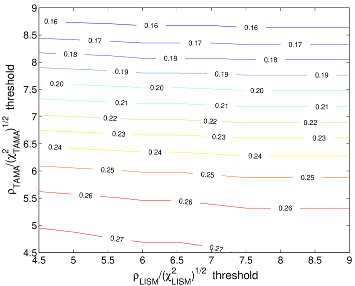
Figure 13: Detection efficiency in the coincidence analysis of sources within 1kpc as a function of TAMA300 and LISM thresholds for $\rho/\sqrt{\chi^{2}}$.

The detection probability $\epsilon$ is derived by the method explained in Section V.2, and is shown in Fig. 13. With the thresholds chosen above, we obtain $\epsilon=0.182$. Using the upper limit to the average number of real events $N$ with $y_{1}$ or $y_{2}$ greater than the threshold, the detection probability $\epsilon$ and the length of data $T=275$ [hours], we obtain an upper limit to the event rate within 1kpc to be $N/(T\epsilon)=0.046$ [1/hour] (CL.= $90\%$).

Unfortunately, this value is not improved from the value obtained by the analysis of the TAMA300 data. The dominant effect that causes the difference in the upper limit for a single-detector analysis and the coincidence analysis comes from the difference in the detection efficiency. The detection efficiency of the coincidence analysis in our case is determined by that of LISM, since LISM has the lower sensitivity. The efficiency of LISM is improved in the case of the coincidence analysis, since the threshold is lowered. However, this does not compensate the difference in the detection efficiency between TAMA300 and LISM. The efficiency of TAMA300 is already nearly 100 % in 1kpc without performing the coincidence analysis. Thus, by taking the coincidence with the detector which has much lower sensitivity, the detection efficiency of the coincidence analysis becomes lower than the case of TAMA300 alone. As a result, the upper limit to the event rate we obtained by the coincidence analysis is less stringent than the one obtained by the analysis of the TAMA300 data.

VII Summary and discussion

In this paper, we performed a coincidence analysis using the data of TAMA300 and LISM taken during DT6 observation in 2001.

We analyzed the data from each detector by matched filtering and obtained event lists. Each event in the lists was characterized by the time of coalescence, masses of the two stars, and the amplitude of events. If any of the events are true gravitational wave events, they should have the consistent values of these parameters in the both event lists. We proposed a method to set coincidence conditions for the source parameters such like the time of coalescence, chirp mass, reduced mass, and the amplitude of events. We took account of the time delay due to the distance between the two detectors, the finite mesh size of the mass parameter space, the difference in the signal amplitudes due to the different sensitivities and antenna patterns of the detectors, and errors in the estimated parameters due to the instrumental noise. Our Monte Carlo studies showed that we would not lose events significantly by imposing the coincidence conditions.

By applying the above method of the coincidence analysis to the event lists of TAMA300 and LISM, we can reduce the number of fake events by a factor $10^{-4}$ compared with the number of fake events before the coincidence analysis. In order to estimate the number of accidental coincidences produced by noise, we used the time shift procedure. We found that the number of events survived after imposing the coincidence conditions is consistent with the expected number of accidental coincidences within the statistical fluctuations. Thus we found no evidence of gravitational wave signals. As discussed in Appendix C, the sidereal time distribution of the survived events were also consistent with the distribution of accidentals.

Finally, we proposed a simple method to set an upper limit to the event rate and applied it to the above results of the coincidence analysis. We obtained an upper limit to the Galactic event rate within 1kpc from the Earth to be 0.046 [1/hour] (90% CL). In our case, since LISM has a much lower sensitivity than TAMA300, we were unable to obtain a more stringent upper limit to the event rate than the one obtained by the single-detector analysis of TAMA300. This is because the detection efficiency in the coincidence analysis is determined by the detector with a lower sensitivity.

However, if we have two detectors that have comparable sensitivities, it is possible to obtain an improved upper limit compared to a single-detector analysis. As an example, let us imagine the case when the sensitivity of LISM is the same as that of TAMA300. The result of Galactic event simulations suggests that the detection efficiency in the case of a single-detector analysis is 0.35, while it improves to 0.48 in the case of a coincidence analysis. These values are translated to upper limits on the Galactic event rate of 0.026 [1/hour] ($90\%$ CL) for the single-detector case and 0.019 [1/hour] ($90\%$ CL) for the two-detector case.

The method of a coincidence analysis and the method to set an upper limit to the event rate proposed here can be readily applied to the case when there are more than two detectors with arbitrary arm directions. Hence these methods will be useful for data analysis for a network of interferometeric gravitational wave detectors in the near future.

Appendix A method to distinguish between real events and non-Gaussian noise

The real data from TAMA300 and LISM contain non-stationary and non-Gaussian noise. One way to remove the influence of such noise is a veto analysis by using the data of various channels which monitor the status of the interferometers and their environments. Such an analysis has been performed using the data of TAMA300 ref:vetoana . However, more efforts will be needed to establish an efficient and faithful veto method.

It was shown that about $20\,\%$ of the data from TAMA300 DT6 contains non-Gaussian noise significantly ref:andoburst . Even if we remove this portion of the data with large non-Gaussian noise, the rest of data may still contain some non-Gaussian noise. It is thus necessary to introduce a method by which we can discriminate the non-Gaussian noise from real gravitational wave signals using the properties of inspiral signals. As one of such methods, the $\chi^{2}$ method was introduced in ref:40m .

In this method, we examine whether the time-frequency behavior of the data is consistent with the expected signal. We divide each template into $n$ mutually independent pieces in the frequency domain, chosen so that the expected contribution to $\rho$ from each frequency band is equal:

$$\tilde{{h}}_{(c,s)}(f)=\tilde{{h}}^{(1)}_{(c,s)}(f)+\tilde{{h}}^{(2)}_{(c,s)}(f)+\cdots+\tilde{{h}}^{(n)}_{(c,s)}(f).$$ (22)

We introduce

$$z^{(i)}_{(c,s)}=(s,{h}^{(i)}_{(c,s)}),\quad\overline{z}^{(i)}_{(c,s)}={1\over n}(s,{h}_{(c,s)}).$$ (23)

Then, $\chi^{2}$ is defined by

$$\chi^{2}=\sum_{i=1}^{n}\left[{\left(z^{(i)}_{(c)}-\overline{z}^{(i)}_{(c)}\right)^{2}+\left(z^{(i)}_{(s)}-\overline{z}^{(i)}_{(s)}\right)^{2}\over\sigma_{(i)}^{2}}\right],$$ (24)

with

$$\sigma_{(i)}^{2}=({h}^{(i)}_{(c)},{h}^{(i)}_{(c)})=({h}^{(i)}_{(s)},{h}^{(i)}_{(s)})={1\over n}.$$ (25)

Provided that the noise is Gaussian, this quantity must satisfy the $\chi^{2}$-statistics with $2n-2$ degrees of freedom and is independent of $\rho=\sqrt{z_{(c)}^{2}+z_{(s)}^{2}}$. For convenience, we use a reduced chi-square defined by $\chi^{2}/(2n-2)$. In this paper, we choose $n=16$.

In the case of TAMA300, it was found that there was a strong tendency that noise events with large $\chi^{2}$ have large values of $\rho$. Since the value of $\chi^{2}$ will be independent of the amplitude of inspiral signals when the parameters such as $t_{c}$, $M$ and $\eta$ of the signal are equal to those of a template ref:grasp , one may expect that we can discriminate real signals from noise events by rejecting events with large $\chi^{2}$, and this method was used in the TAMA300 DT2 analysis ref:DT2 .

However, in reality, since we perform analysis on a discrete $t_{c}$ and a discrete mass parameter space, the parameters of a signal do not coincide with those of a template in general. We have found in the analysis of the TAMA300 DT4 data in 2000 that this difference produces a large value of $\chi^{2}$ when the $SNR$ of an event is very large even if the event is real ref:TAMAinspiral . Thus, if we apply a threshold to the value of $\chi^{2}$ to reject noise events, we may lose real events with large $SNR$. This is a serious problem since an event with a large $SNR$ has a high statistical significance of it to be real. This lead us to introduce a different rejection criterion when we performed an inspiraling wave search with the TAMA300 DT4 data ref:TAMAinspiral , namely, a threshold on the value of $\rho/\sqrt{\chi^{2}}$. By Galactic event simulations, we found that this new criterion can give a better detection efficiency of the Galactic events without losing strong amplitude events.

Here we examine whether the $\rho/\sqrt{\chi^{2}}$ selection is useful also in the case of the TAMA300 DT6 data. For comparison, the detection efficiency for a simple $\chi^{2}$ threshold is shown in Fig. 14.

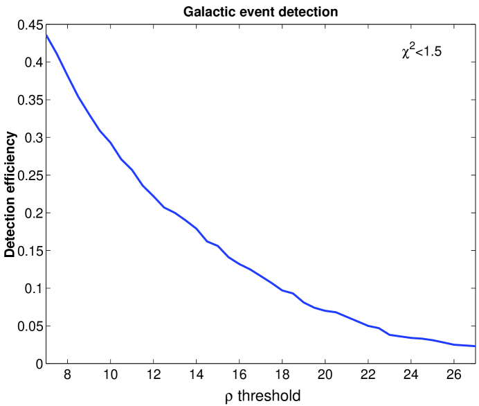
Figure 14: Detection efficiency for a $\chi^{2}$ threshold. In this figure, the threshold is set to $\chi^{2}=1.5$.

For the $\chi^{2}<1.5$ threshold, using 287.6 hours of the data, the false alarm rate $2.0$ [1/yr] determines the $SNR$ threshold to be $\rho=12.5$. This gives the detection efficiency of $0.213$. On the other hand, as discussed in Section IV, the detection efficiency in the case of the $\rho/\sqrt{\chi^{2}}$ threshold is $0.263$ for the same false alarm rate, $2.0$ [1/yr]. We thus find that we have a better efficiency for the $\rho/\sqrt{\chi^{2}}$ threshold, although the gain of efficiency is not very large. However, the important point is that we have much larger detection efficiency for signals with large $SNR$.

Appendix B Different choice of $\Delta t$

In this appendix, we consider the case of a different choice of the length of duration $\Delta t$ to find local maximum of matched filtering output (see III.2), to see if our conclusion is affected by a different choice of $\Delta t$.

Here we adopt $\Delta t=3.28$sec. In this case, the total number of events is found to be 158,437 for TAMA300 and 142,465 for LISM. The numbers of events survived after each step of the coincidence selections are given in Table 5. The corresponding estimated numbers of accidentals are also shown. The scatter plots of these selected events are shown in Figs. 15 and 16. We see that the number of coincident events is consistent with the number of accidentals within the standard deviation, in agreement with our conclusion given in the main text of this paper.

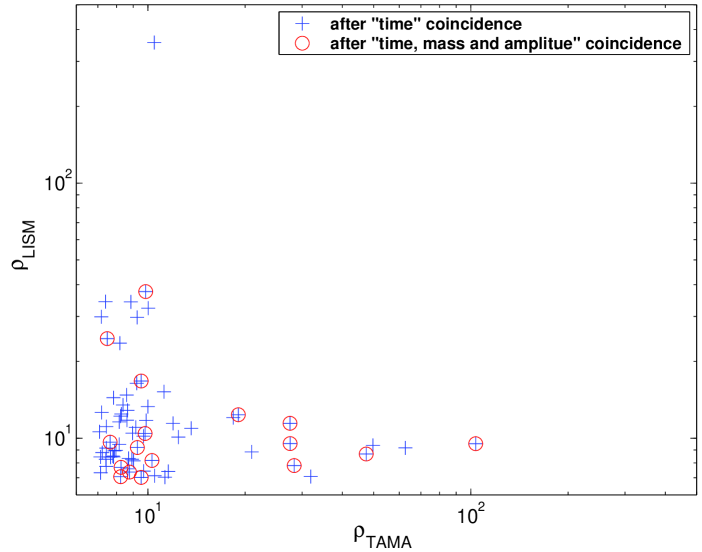
Figure 15: ($\rho_{\mbox{\rm\tiny TAMA}}$,$\rho_{\mbox{\rm\tiny LISM}}$) scatter plots in the case $\Delta t=3.28$sec. The crosses (+) are the events survived after the time selection, and the circled crosses ($\oplus$) are the events survived after the time, mass and amplitude selections.

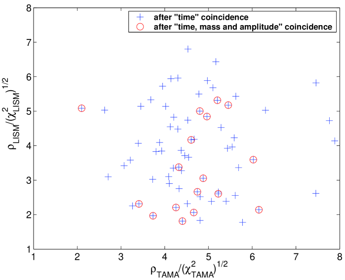
Figure 16: ($\rho_{\mbox{\rm\tiny TAMA}}/\sqrt{\chi^{2}_{\mbox{\rm\tiny TAMA}}}$ ,$\rho_{\mbox{\rm\tiny LISM}}/\sqrt{\chi^{2}_{\mbox{\rm\tiny LISM}}}$) scatter plots in the case $\Delta t=3.28$sec, The crosses (+) are the events survived after the time selection, and the circled crosses ($\oplus$) are the events survived after the time, mass and amplitude selections.

Results of independent matched filtering searches
	TAMA300	LISM
Number of events	158,437	142,465
Results of coincidence analysis
	$n_{\rm obs}$	$\bar{n}_{\rm acc}\pm\bar{\sigma}_{\rm acc}$
after time selection	70	$75.0\pm 8.6$
after time and mass selection	18	$18.8\pm 4.1$
after time, mass and amplitude selection	17	$17.9\pm 3.8$

Table 5: Results of coincidence analysis in the case $\Delta t=3.28$sec. $n_{\rm obs}$ is the number of coincidence events. $\bar{n}_{\rm acc}$, $\bar{\sigma}_{\rm acc}$ are the estimated number of accidental coincidence and its variance.

Appendix C Sidereal time distribution

In this appendix, we examine the sidereal time distribution of the events. In Fig. 17 (a), we plot the number of coincident events as a function of the local sidereal hour at the location of TAMA300. The estimated number of accidental coincidences are also plotted, which are obtained by the same time shift method used in Section V.3 but for data within each bin of the sidereal hour. If the gravitational wave sources are sharply concentrated in the Galactic disk, we would detect more events when the zenith direction of the detector coincides with the direction to the Galactic plane than the rest of time. The zenith direction faces to the Galactic disk at around 6:00 and 18:00 in the sidereal hour. Since LISM is only sensitive to sources within a few kpc, we may not be able to see any significant excess of the events in the Galactic disk within this distance unless the concentration of the sources to the Galactic disk is very strong. Even in this case, it is useful to investigate the sidereal time distribution to look for signatures of real events.

We find that the distribution of coincident events is consistent with accidentals, although there are a few hours in which the agreement is not very good. Thus, we conclude that the result of the sidereal hour distribution is consistent with the number of accidentals, and there is no signature of gravitational wave event.

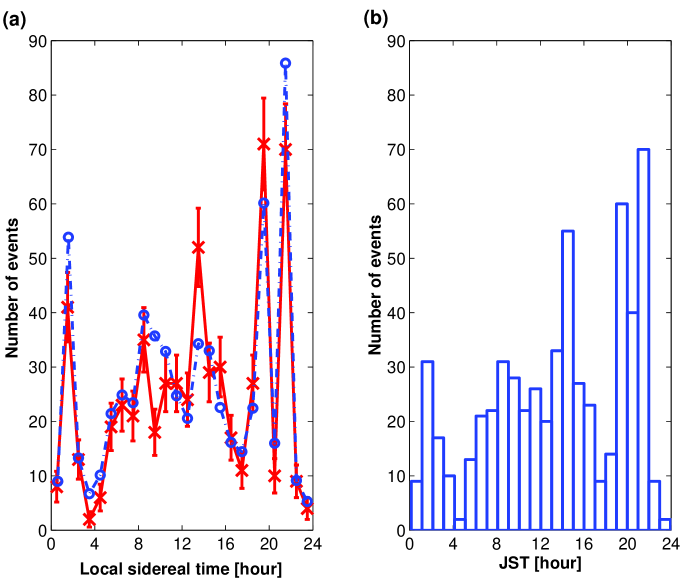
Figure 17: (a) The event distribution as a function of the local sidereal time. The solid line represents the number of coincident events per one sidereal hour. The dot-dashed line represents the estimated number of accidentals. (b) The number of coincident events as a function of the Japanese Standard Time.

In Fig. 17 (b), we also plot the number of coincident events as a function of the Japanese Standard Time (JST). Since the deviation of the local sidereal time from JST is not very large during the period of observation, this figure is very similar to Fig. 17 (a). The reason that there are many coincident events during 20:00 to 22:00 JST is due to a large number of events recorded by LISM during that period. During the DT6 observation, there were some activities in the Kamioka mine from 20:00 to 22:00 JST, and trucks went through the tunnel of the mine during that period. We suspect this caused fake events in LISM.

Appendix D Parameter estimation errors induced by detector noise

In this appendix, we briefly review the theory of the parameter estimation error developed in ref:Cutler . This is used in determining the parameter windows for the coincidence analysis in this paper.

In the matched filtering, for a given incident gravitational wave, different realizations of the noise will give rise to somewhat different best-fit parameters. For a large $SNR$, the best-fit parameters will have Gaussian distributions centered on the correct values. Specifically, let $\tilde{\theta^{i}}$ be the correct values of the parameters, and let $\tilde{\theta^{i}}+\Delta\theta^{i}$ be the best-fit parameters in the presence of a realization of noise. Then for large $SNR$, the parameter estimation errors $\Delta\theta^{i}$ have the Gaussian probability distribution

$$p(\Delta\theta^{i})=\mathcal{N}e^{-\frac{1}{2}\Gamma_{ij}{\Delta\theta^{i}\Delta\theta^{j}}}.$$ (26)

where $\Gamma_{ij}$ is the called Fisher Information matrix defined by

$$\Gamma_{ij}\equiv\Big{(}\frac{\partial h}{\partial\theta^{i}},\frac{\partial h}{\partial\theta^{j}}\Big{)},$$ (27)

and $\mathcal{N}=\sqrt{{\rm det}(\mathbf{\Gamma}/2\pi)}$ is the normalization factor. It follows that the root-mean-square errors in $\theta^{i}$ is given by

$$\sigma_{i}=\sqrt{((\Delta\theta^{i})^{2})}=\sqrt{\Sigma^{ii}},$$ (28)

where $\mathbf{\Sigma}\equiv\mathbf{\Gamma}^{-1}$, and the correlation coefficient between parameters $\theta^{i}$ and $\theta^{j}$ is given by

$$c^{ij}=\frac{<\Delta\theta^{i}\Delta\theta^{j}>}{\sigma_{i}\sigma_{j}}=\frac{\Sigma^{ij}}{\sqrt{\Sigma^{ii}\Sigma^{jj}}}.$$ (29)

By definition, each $c^{ij}$ lies in the range $(-1,1)$.

As given in Section III.1, an inspiraling signal in the frequency domain is given by

$$\tilde{h}(f)=\mathcal{A}f^{-7/6}e^{i\psi(f)}.$$ (30)

Here we consider the phase $\psi(f)$ up only to the second post-Newtonian order but including the effect of the spins of stars. Note that this is slightly different from the template formula (4) used in our analysis. The phase $\psi(f)$ is given by

$$\psi(f) = 2\pi ft_{c}-\phi_{c}-\frac{\pi}{4}+\frac{3}{128}(\pi\mathcal{M}f)^{-5/3}\Big{[}1+\frac{20}{9}\Big{(}\frac{743}{336}+\frac{11}{4}\eta\Big{)}(\pi Mf)^{2/3}-4(4\pi-\beta)(\pi Mf)$$ (31)

$${}+10\Big{(}\frac{3058673}{1016064}+\frac{5429}{1008}\eta+\frac{617}{144}\eta^{2}-\sigma\Big{)}(\pi Mf)^{4/3}\Big{]}.$$

In the above, $\beta$ is the spin-orbit parameter given by

$$\beta=\frac{1}{12}\sum_{i=1}^{2}[113(m_{i}/M)+75\eta]\hat{\mathbf{L}}\cdot\mbox{\boldmath$\chi$}_{i},$$ (32)

and $\mbox{\boldmath$\chi$}_{i}=\mathbf{S}_{i}/m^{2}_{i}$, and $\mathbf{S}_{i}$ is the spin angular momentum of each star, and $\hat{\mathbf{L}}$ is the unit vector along the orbital angular momentum vector. The spin-spin parameter $\sigma$ is given by

$$\sigma=\frac{\eta}{48}(-247\mbox{\boldmath$\chi$}_{1}\cdot\mbox{\boldmath$\chi$}_{2}+721\hat{\mathbf{L}}\cdot\mbox{\boldmath$\chi$}_{1}\hat{\mathbf{L}}\cdot\mbox{\boldmath$\chi$}_{2}).$$ (33)

We define

$$\rho^{2}=4\mathcal{A}^{2}\int^{f_{\rm max}}_{0}\frac{f^{-7/3}}{S_{n}(f)}df.$$ (34)

We also define the frequency moments $\bar{f}_{\alpha}$ of the noise spectrum density:

$$f_{7/3} \equiv \int_{0}^{f_{\rm max}}df\quad[f^{7/3}S_{n}(f)]^{-1}$$ (35)

$$\bar{f}_{\alpha} \equiv f_{7/3}^{-1}\int_{0}^{f_{\rm max}}df\quad[f^{\alpha}S_{n}(f)]^{-1}.$$ (36)

In order to evaluate the Fisher matrix, we calculate the derivatives of $\tilde{h}(f)$ with respect to the seven parameters

$$\mbox{\boldmath$\theta$}=(\ln{\mathcal{A}},f_{0}t_{c},\phi_{c},\ln{\cal M},\ln\eta,\beta,\sigma),$$ (37)

where $f_{0}$ is a fiducial frequency which is taken to be the frequency at which $S_{n}(f)$ becomes minimum. We obtain

$$\frac{\partial\tilde{h}(f)}{\partial\ln\mathcal{A}} = \tilde{h}(f),$$

$$\frac{\partial\tilde{h}(f)}{\partial f_{0}t_{c}} = 2\pi i\Big{(}\frac{f}{f_{0}}\Big{)}\ \tilde{h}(t),$$

$$\frac{\partial\tilde{h}(f)}{\partial\phi_{c}} = -i\tilde{h}(f),$$

$$\frac{\partial\tilde{h}(f)}{\partial\ln\mathcal{M}} = -\frac{5i}{128}(\pi\mathcal{M}f)^{-5/3}\big{\{}1+A_{4}(\pi Mf)^{2/3}-B_{4}(\pi Mf)+C_{4}(\pi Mf)^{4/3}\big{\}}\ \tilde{h}(f),$$

$$\frac{\partial\tilde{h}(f)}{\partial\ln\eta} = -\frac{i}{96}(\pi\mathcal{M}f)^{-5/3}\big{\{}A_{5}(\pi Mf)^{2/3}-B_{5}(\pi Mf)+C_{5}(\pi Mf)^{4/3}\big{\}}\ \tilde{h}(f),$$

$$\frac{\partial\tilde{h}(f)}{\partial\beta} = \frac{3i}{32}\eta^{-3/5}(\pi\mathcal{M}f)^{-2/3}\tilde{h}(f),$$

$$\frac{\partial\tilde{h}(f)}{\partial\sigma} = -\frac{15i}{64}\eta^{-4/5}(\pi\mathcal{M}f)^{-1/3}\tilde{h}(f).$$ (38)

Here we have defined

$$A_{4} = \frac{4}{3}\Big{(}\frac{743}{336}+\frac{11}{4}\eta\Big{)},$$

$$B_{4} = \frac{8}{5}(4\pi-\beta),$$

$$C_{4} = 2\Big{(}\frac{3058673}{1016064}+\frac{5429}{1008}\eta+\frac{617}{144}\eta^{2}-\sigma\Big{)},$$ (39)

and

$$A_{5} = \frac{743}{168}-\frac{33}{4}\eta,$$

$$B_{5} = \frac{27}{5}(4\pi-\beta),$$

$$C_{5} = 18\Big{(}\frac{3058673}{1016064}+\frac{5429}{4032}\eta+\frac{617}{96}\eta^{2}-\sigma\Big{)}.$$ (40)

Finally, the components of $\Gamma$ can be obtained by evaluating Eq. (27). They can be expressed in terms of the parameters $\theta$, the signal-to-noise ratio $\rho$, and the frequency moments $\bar{f}_{\beta}$. The components of $\Gamma_{ij}$ are given by

$$\Gamma_{\ln\mathcal{A}j} = \delta_{\ln\mathcal{A}j}\rho^{2},\qquad(j=\ln\mathcal{A},f_{0}t_{c},\phi_{c},\ln\mathcal{M},\ln\eta,\sigma,\beta),$$ (41)

$$\Gamma_{t_{c}t_{c}} = (2\pi)^{2}\frac{1}{f_{0}}\bar{f}_{1/3}\ \rho^{2},$$ (42)

$$\Gamma_{t_{c}\phi_{c}} = -2\pi\frac{1}{f_{0}}\bar{f}_{4/3}\ \rho^{2},$$ (43)

$$\Gamma_{t_{c}\ln\mathcal{M}} = -\frac{5\pi}{64f_{0}}(\pi\mathcal{M})^{-5/3}\Big{(}\bar{f}_{3}+A_{4}(\pi M)^{2/3}-B_{4}(\pi M)\bar{f}_{2}+C_{4}(\pi M)^{4/3}\bar{f}_{5/3}\Big{)}\ \rho^{2},$$ (44)

$$\Gamma_{t_{c}\ln\eta} = -\frac{\pi}{48f_{0}}(\pi\mathcal{M})^{-5/3}\Big{(}A_{5}(\pi M)^{2/3}-B_{5}(\pi M)\bar{f}_{2}+C_{5}(\pi M)^{4/3}\bar{f}_{5/3}\Big{)}\ \rho^{2},$$ (45)

$$\Gamma_{t_{c}\ln\beta} = \frac{3\pi}{16f_{0}}\eta^{-3/5}(\pi\mathcal{M})^{-2/3}\bar{f}_{2}\ \rho^{2},$$ (46)

$$\Gamma_{t_{c}\sigma} = -\frac{15\pi}{32f_{0}}\eta^{-4/5}(\pi\mathcal{M})^{-1/3}\bar{f}_{5/3}\ \rho^{2},$$ (47)

$$\Gamma_{\phi_{c}t_{c}} = \Gamma_{t_{c}\phi_{c}},$$ (48)

$$\Gamma_{\phi_{c}\phi_{c}} = \rho^{2},$$ (49)

$$\Gamma_{\phi_{c}\ln\mathcal{M}} = \frac{5}{128}(\pi\mathcal{M})^{-5/3}\Big{(}\bar{f}_{4}+A_{4}(\pi M)^{2/3}\bar{f}_{10/3}-B_{4}(\pi M)\bar{f}_{3}+C_{4}(\pi M)^{4/3}\bar{f}_{8/3}\Big{)}\ \rho^{2},$$ (50)

$$\Gamma_{\phi_{c}\ln\eta} = \frac{1}{96}(\pi\mathcal{M})^{-5/3}\Big{(}A_{5}(\pi M)^{2/3}\bar{f}_{10/3}-B_{5}(\pi M)\bar{f}_{3}+C_{5}(\pi M)^{4/3}\bar{f}_{8/3}\Big{)}\ \rho^{2},$$ (51)

$$\Gamma_{\phi_{c}\beta} = -\frac{3}{32}\eta^{-3/5}(\pi\mathcal{M})^{-2/3}\bar{f}_{3}\ \rho^{2},$$ (52)

$$\Gamma_{\phi_{c}\sigma} = \frac{15}{64}\eta^{-4/5}(\pi\mathcal{M})^{-1/3}\bar{f}_{8/3}\ \rho^{2},$$ (53)

$$\Gamma_{\ln\mathcal{M}t_{c}} = \Gamma_{t_{c}\ln\mathcal{M}},$$ (54)

$$\Gamma_{\ln\mathcal{M}\phi_{c}} = \Gamma_{\phi_{c}\ln\mathcal{M}},$$ (55)

$$\Gamma_{\ln\mathcal{M}\ln\mathcal{M}} = \frac{25}{16384(\pi\mathcal{M})^{10/3}}\Big{(}A_{4}^{2}(\pi M)^{4/3}\bar{f}_{17/3}\bar{f}_{13/3}+2A_{4}(\pi M)^{2/3}\Big{\{}\bar{f}_{15/3}-B_{4}\pi M\bar{f}_{4}$$ (56)

$${}+C_{4}(\pi M)^{4/3}\bar{f}_{11/3}+\pi M(B_{4}^{2}\pi M\bar{f}_{11/3}-2B_{4}(\bar{f}_{14/3}$$

$${}+C_{4}(\pi M)^{4/3}\bar{f}_{10/3}))\Big{\}}\Big{)}\ \rho^{2},$$

$$\Gamma_{\ln\mathcal{M}\ln\eta} = \frac{1}{12288\pi^{8/3}\mathcal{M}^{10/3}}\Big{(}5M^{2/3}(A_{5}\Big{\{}\bar{f}_{15/3}+A_{4}(\pi M)^{2/3}\bar{f}_{13/3}-B_{4}\pi M\bar{f}_{4}$$ (57)

$${}+C_{4}(\pi M)^{4/3}\bar{f}_{11/3}+(\pi M)^{1/3}(C_{5}(\pi M)^{1/3}(\bar{f}_{13/3}+A_{4}(\pi M)^{2/3}\bar{f}_{11/3}$$

$${}-B_{4}\pi M\bar{f}_{10/3}+C_{4}(\pi M)^{4/3}\bar{f}_{3})-B_{5}(\bar{f}_{114/3}+A_{4}(\pi M)^{2/3}\bar{f}_{4}$$

$${}-B_{4}\pi M\bar{f}_{11/3}+C_{4}(\pi M)^{4/2}\bar{f}_{10/3})))\Big{\}}\Big{)}\ \rho^{2},$$

$$\Gamma_{\ln\mathcal{M}\beta} = -\frac{15}{4096}\eta^{-3/5}(\pi\mathcal{M})^{-7/3}\Big{(}\bar{f}_{14/3}+A_{4}(\pi M)^{2/3}\bar{f}_{4}-B_{4}(\pi M)\bar{f}_{11/3}$$ (58)

$${}+C_{4}(\pi M)^{4/3}\bar{f}_{10/3}\Big{)}\ \rho^{2},$$

$$\Gamma_{\ln\mathcal{M}\sigma} = \frac{75}{8192}\eta^{-4/5}(\pi\mathcal{M})^{-2}\Big{(}\bar{f}_{13/3}+A_{4}(\pi M)^{2/3}\bar{f}_{11/3}-B_{4}(\pi M)\bar{f}_{10/3}$$ (59)

$${}+C_{4}(\pi M)^{4/3}\bar{f}_{3}\Big{)}\ \rho^{2},$$

$$\Gamma_{\ln\eta t_{c}} = \Gamma_{t_{c}\ln\eta},$$ (60)

$$\Gamma_{\ln\eta\phi_{c}} = \Gamma_{\phi_{c}\ln\eta},$$ (61)

$$\Gamma_{\ln\eta\ln\mathcal{M}} = \Gamma_{\ln\mathcal{M}\ln\eta},$$ (62)

$$\Gamma_{\ln\eta\ln\eta} = \frac{1}{9216\pi^{2}\mathcal{M}^{10/3}}\Big{(}M^{4/3}\Big{\{}A_{5}^{2}\bar{f}_{13/3}-2A_{5}B_{5}(\pi M)^{1/3}\bar{f}_{4}+B_{5}^{2}(\pi M)^{2/3}\bar{f}_{11/3}$$ (63)

$${}+2A_{5}B_{5}(\pi M)^{2/3}\bar{f}_{11/3}-2B_{5}C_{5}\pi M\bar{f}_{10/3}+C_{5}^{2}(\pi M)^{4/3}\bar{f}_{3}\Big{\}}\Big{)}\ \rho^{2},$$

$$\Gamma_{\ln\eta\beta} = -\frac{1}{1024}\eta^{-3/5}(\pi\mathcal{M})^{-7/3}\Big{(}A_{5}(\pi M)^{2/3}\bar{f}_{4}-B_{5}(\pi M)\bar{f}_{11/3}$$ (64)

$${}+C_{5}(\pi M)^{4/3}\bar{f}_{10/3}\Big{)}\ \rho^{2},$$

$$\Gamma_{\ln\eta\sigma} = \frac{5}{2048}\eta^{-4/5}(\pi\mathcal{M})^{-2}\Big{(}A_{5}(\pi M)^{2/3}\bar{f}_{11/3}-B_{5}(\pi M)\bar{f}_{10/3}$$ (65)

$${}+C_{5}(\pi M)^{4/3}\bar{f}_{3}\Big{)}\ \rho^{2},$$

$$\Gamma_{\beta t_{c}} = \Gamma_{t_{c}\beta},$$ (66)

$$\Gamma_{\beta\phi_{c}} = \Gamma_{\phi_{c}\beta},$$ (67)

$$\Gamma_{\beta\ln\mathcal{M}} = \Gamma_{\ln\mathcal{M}\beta},$$ (68)

$$\Gamma_{\beta\ln\eta} = \Gamma_{\ln\eta\beta},$$ (69)

$$\Gamma_{\beta\beta} = \frac{9}{1024}\eta^{-6/5}(\pi\mathcal{M})^{-4/3}\bar{f}_{11/3}\ \rho^{2},$$ (70)

$$\Gamma_{\beta\sigma} = -\frac{45}{2048}\eta^{-7/5}(\pi\mathcal{M})^{-1}\bar{f}_{10/3}\ \rho^{2},$$ (71)

$$\Gamma_{\sigma t_{c}} = \Gamma_{t_{c}\sigma},$$ (72)

$$\Gamma_{\sigma\phi_{c}} = \Gamma_{\phi_{c}\sigma},$$ (73)

$$\Gamma_{\sigma\ln\mathcal{M}} = \Gamma_{\ln\mathcal{M}\sigma},$$ (74)

$$\Gamma_{\sigma\ln\eta} = \Gamma_{\ln\eta\sigma},$$ (75)

$$\Gamma_{\sigma\beta} = \Gamma_{\beta\sigma},$$ (76)

$$\Gamma_{\sigma\sigma} = \frac{225}{4096}\eta^{-8/5}(\pi\mathcal{M})^{-2/3}\bar{f}_{3}\ \rho^{2}.$$ (77)

It is ensured by these formulas that the eigenvalues of the Fisher matrix are always positive definite.

The variance-covariance matrix $\Sigma^{ij}$ can now be obtained from $\mbox{\boldmath$\Sigma$}=\mbox{\boldmath$\Gamma$}^{-1}$, and the root-mean square errors and the correlation coefficients are computed from Eqs. (28) and (29).

For example, using a typical noise spectrum density of TAMA300, the root-mean square errors of the parameters in the case $\rho=10$ and $\beta=\sigma=0$ are evaluated to be $\Delta{\cal A}^{\rm TAMA}/{\cal A}^{\rm TAMA}=0.10$, $\Delta t_{c}^{\rm TAMA}=0.65$msec, $\Delta\phi_{c}^{\rm TAMA}=6.88$radians, $\Delta\mathcal{M}^{\rm TAMA}/\mathcal{M}^{\rm TAMA}=1.43\times 10^{-2}$, and $\Delta\eta^{\rm TAMA}/\eta^{\rm TAMA}=2.47\times 10^{-1}$.

References

- (1) B. Abbott et al. (The LIGO Scientific Collaboration), Nucl. Instrum. Meth. A517, 154 (2004) , gr-qc/0308043.
- (2) B.Caron et al., in Gravitational Wave Experiments, edited by E. Coccia, G. Pizzella, and F. Ronga, (World Scientific, Singapore, 1995).
- (3) K. Danzmann et al.,in Gravitational Wave Experiments, edited by E. Coccia,G. Pizzella, and F. Ronga,(World Scientific, Singapore,1995).
- (4) S. Kawamura and N. Mio eds., Gravitational Wave Detection II ,(Proceedings of the 2nd TAMA workshop on Gravitational Wave Detection), (Univ. Acad. Press, Tokyo, 2000).
- (5) M. Ando et al., (The TAMA Collaboration), Phys.Rev.Lett., 86, 3950 (2001).
- (6) D. Nicholson et al., Phys. Lett. A, 218, 175 (1996).
- (7) B. Allen et al., Phys. Rev. Lett. 83, 1489 (1999).
- (8) H. Tagoshi et al., (The TAMA Collaboration), Phys. Rev. D 63, 062001 (2001).
- (9) B. Abbott et al., (The LIGO Scientific Collaboration), Phys. Rev. D 69, 122001 (2004) ..
- (10) P. Astone et al. (International Gravitational Event Collaboration), Phys. Rev. D 68, 022001 (2003).
- (11) S. Sato et al., Applied Optics 39, 4616 (2000).
- (12) S. Sato et al. (The LISM Collaboration), Phys. Rev. D 69, 102005 (2004) .
- (13) S. Droz, D.J. Knapp, E. Poisson, and B.J. Owen, Phys. Rev. D59, 124016 (1999).
- (14) L. Blanchet, T. Damour, B.R. Iyer, C.M. Will, and A.G. Wiseman, Phys. Rev. Lett. 74, 3515 (1995); L. Blanchet, B.R. Iyer, C.M. Will, and A.G. Wiseman, Class. Quant. Grav. 13, 575 (1996); L. Blanchet, Phys. Rev. D54, 1417 (1996).
- (15) T. Tanaka and H. Tagoshi, Phys. Rev. D 62, 082001 (2000).
- (16) S.J. Curran and D.R. Lorimer, Mon. Not. R. Astron. Soc. 276, 347 (1995).
- (17) For example, Particle Data Group, Review of Particle Physics, Phys. Lett. B204 (1988), 81; ibid. Euro. Phys. J. C3, (1998), 172-177, and references cited there.
- (18) E. Amaldi et al.,Astron. Astrophys. 216, 325 (1989).
- (19) P. Astone et al., Phys. Rev. D 59, 122001 (1999).
- (20) M. Ando et al., in preparation.
- (21) B. Allen ed. ”Users manual of GRASP: a data analysis package for gravitational wave detection”, version 1.9.4. , B. Allen, accepted by Phys. Rev. D http://arxiv.org/gr-qc/0405045.
- (22) H. Tagoshi, H. Takahashi et al.,in preparation.
- (23) C. Cutler and É. E. Flanagan, Phys. Rev. D 49, 082001 (1994).
- (24) N. Kanda et al., work in progress.