Gravitational-wave astronomy: the high-frequency window

Abstract

As several large scale interferometers are beginning to take data at sensitivities where astrophysical sources are predicted, the direct detection of gravitational waves may well be imminent. This would (finally) open the long anticipated gravitational-wave window to our Universe, and should lead to a much improved understanding of the most violent processes imaginable; the formation of black holes and neutron stars following core collapse supernovae and the merger of compact objects at the end of binary inspiral. Over the next decade we can hope to learn much about the extreme physics associated with, in particular, neutron stars.

This contribution is divided in two parts. The first part provides a text-book level introduction to gravitational radiation. The key concepts required for a discussion of gravitational-wave physics are introduced. In particular, the quadrupole formula is applied to the anticipated “bread-and-butter” source for detectors like LIGO, GEO600, EGO and TAMA300: inspiralling compact binaries. The second part provides a brief review of high frequency gravitational waves. In the frequency range above (say) 100 Hz, gravitational collapse, rotational instabilities and oscillations of the remnant compact objects are potentially important sources of gravitational waves. Significant and unique information concerning the various stages of collapse, the evolution of protoneutron stars and the details of the supranuclear equation of state of such objects can be drawn from careful study of the gravitational-wave signal. As the amount of exciting physics one may be able to study via the detections of gravitational waves from these sources is truly inspiring, there is strong motivation for the development of future generations of ground based detectors sensitive in the range from hundreds of Hz to several kHz.

1 Introduction

One of the central predictions of Einsteins’ general theory of relativity is that gravitational waves will be generated as masses are accelerated. Despite decades of effort these ripples in spacetime have still not been observed directly. Yet we have strong indirect evidence for their existence from the excellent agreement between the observed inspiral rate of the binary pulsar PSR1913+16 and the theoretical prediction (better than 1% in the phase evolution). This provides confidence in the theory and suggests that “gravitational-wave astronomy” should be viewed as a serious proposition. Provided that i) detectors with the required sensitivity can be constructed, and ii) the significant data analysis challenge can be dealt with, this new window to the Universe promises to bring unprecedented insights into the most violent events imaginable; supernova explosions, binary mergers and the big bang itself. A key reason for this expectation follows from a comparison between gravitational and electromagnetic waves:

• While electromagnetic waves are radiated by individual particles, gravitational waves are due to non-spherical bulk motion of matter. In essence, this means that the information carried by electromagnetic waves is stochastic in nature, while the gravitational waves provide insights into coherent mass currents.

• The electromagnetic waves will have been scattered many times. In contrast, gravitational waves interact weakly with matter and arrive at the Earth in pristine condition. This means that gravitational waves can be used to probe regions of space that are opaque to electromagnetic waves, It is, of course, a blessing in disguise since the weak interaction with matter also makes the gravitational waves fiendishly hard to detect.

• Standard astronomy is based on deep imaging of small fields of view, while gravitational-wave detectors cover virtually the entire sky.

• Electromagnetic radiation has a wavelength smaller than the size of the emitter, while the wavelength of a gravitational wave is usually larger than the size of the source. This means that we cannot use gravitational-wave data to create an image of the source. In fact, gravitational-wave observations are more like audio than visual.

Morale: Gravitational waves carry information which would be very difficult to glean by other means. By analysing gravitational-wave data we can expect to learn a lot about the extreme physics governing compact objects. This should lead to answers to many outstanding questions in astrophysics, for example,

• What is the black-hole population of the Universe? Observations of the nonlinear spacetime dynamics associated with binary merger, as well as the quasinormal mode (QNM) ringing which is likely to dominate the radiation at late times, should provide direct proof of the presence of a black hole, as well as a measure of it’s mass and spin.

• Are astrophysical black holes, indeed, described by the Kerr metric? By studying the inspiral of a low-mass object into a supramassive black hole (as anticipated at the centre of most galaxies) we can hope to construct a detailed map of the exterior black-hole spacetime.

• What is the supranuclear neutron star equation of state? This is a very difficult question, which potentially involves an understanding of the role of exotic phases of matter, like deconfined quarks, superfluidity/conductivity, extreme magnetic fields etcetera. At an immediate level, gravitational-wave observations of the various oscillation modes of a compact star may be used to solve the “inverse problem” for parameters like the mass and the radius of the star. At a more subtle level, the spectrum of the star depends on the internal physics. For example, strong composition gradients which affect the gravity g-modes significantly, and superfluidity which leads to the existence of new classes of oscillations associated with the more or less decoupled additional degrees of freedom of such a system. Finally, the internal physics also plays a crucial role in determining the extent to which various rotational instabilities will be able to grow to an interesting amplitude. In the case of the Coriolis driven r-modes, their instability may be severely suppressed by the presence of hyperons in the stars core. A key role is also played by the internal magnetic fields.

At the time of writing, the new generation of interferometric gravitational-wave detectors (in particular LIGO and GEO600) is already collecting data at a sensitivity at least one order of magnitude better than that of the operating resonant detectors. In the first instance, the broadband detectors will be sensitive in a range of frequencies between 50 and a few hundred Hz. This frequency window is of great interest since an inspiraling compact binary will move through it during the last few minutes before merger. Such sources are the natural “bread and butter” source for the detectors. The next generation of interferometers will broaden the bandwidth somewhat but will still not be very sensitive to frequencies above 500-600 Hz, unless they are operated in a narrow-band configuration ThorneCutler ; GEO600 . There are also interesting suggestions for wide band resonant detectors in the kHz band Cerdonio . The move towards higher frequencies is driven by the wealth of exciting sources that radiate in the range from a few hundred Hz up to several kHz.

Our contribution to these proceedings is divided in two parts. The first part describes gravitational-wave physics at an introductory level. The second part provides a brief review of the main sources that radiate in the frequency band above a few hundred Hz. We believe that these sources are the natural targets for a third generation of ground based detectors. As we will discuss, there are a variety of sources associated with very interesting physics in this high-frequency window. These sources clearly deserve special attention, and if either resonant or narrow-band interferometers can achieve the required sensitivity, a plethora of unique information can be gathered.

2 Einstein’s elusive waves

The aim of the first part of our contribution is to provide a condensed text-book level introduction to gravitational waves. Although in no sense complete this description should prepare the reader for the discussion of high-frequency sources which follows.

2.1 The nature of the waves

The first aspect of gravitational waves that we need to appreciate is their tidal nature. This is important because it implies that they can only be measured through the relative motion of bodies. That this should be the case is easy to understand. In general relativity we can always construct a local inertial frame associated with a given observer. In this local frame, spacetime will by construction be flat which means that we cannot hope to observe the local deformations which would correspond to a gravitational wave.

Figure 1: An illustration of the two test particles discussed in the text. If a gravitational wave passes through, particle $A$ will observe particle $B$ oscillating back and forth.

Consider two test particles, $A$ and $B$, that are initially at rest. Assume that they are separated by a purely spatial vector $\xi^{j}$ (hereafter latin indices are spatial and run from 1–3, while greek indices are spacetime and run from 0–4), and use the local inertial frame in which particle $A$ remains at the origin for the calculation. In this case the equation of geodesic deviation can be written

$$\frac{\partial^{2}\xi^{j}}{\partial t^{2}}=-R^{j}_{\ 0k0}\xi^{k}$$ (1)

where $R_{\mu\nu\delta\gamma}$ is the Riemann tensor. Here it represents the curvature induced by the gravitational wave. Letting $\xi^{j}=x_{0}^{j}+\delta x^{j}$, with $\delta x^{j}$ the small displacement away from the original position, we get

$$\frac{\partial^{2}\delta x^{j}}{\partial t^{2}}\approx-R^{j}_{\ 0k0}x_{0}^{k}=-R_{j0k0}x_{0}^{k}$$ (2)

Now it is natural to define the gravitational wave-field $h_{jk}$ through

$$R_{j0k0}\equiv-{1\over 2}{\partial^{2}h_{jk}\over\partial t^{2}}\longrightarrow{\partial^{2}\delta x_{j}\over\partial t^{2}}\approx{1\over 2}{\partial^{2}h_{jk}\over\partial t^{2}}x_{0}^{k}$$ (3)

which integrates to

$$\delta x_{j}={1\over 2}h_{jk}x_{0}^{k}\quad\mbox{or}\quad h\approx{\Delta L\over L}$$ (4)

where $h$ is the dimensionless gravitational-wave strain. From this exercise we learn that, in order to detect gravitational waves we need to monitor (with extreme precision) the relative motion of test masses.

Figure 2: The two gravitational-wave polarisations $h_{+}$ and $h_{\times}$.

Let us now assume that the waves propagate in the $z$-direction, i.e. that we have $h_{jk}=h_{jk}(t-z)$. Then one can show that we have only two independent components;

$$h_{+}=h_{xx}^{\mathrm{TT}}=-h_{yy}^{\mathrm{TT}}\qquad h_{\times}=h_{xy}^{\mathrm{TT}}=h_{yx}^{\mathrm{TT}}$$ (5)

What effect does $h_{+}$ have on matter? Consider a particle initially located at $(x_{0},y_{0})$ and let $h_{\times}=0$ to find that

$$\delta x = {1\over 2}h_{+}x_{0}$$ (6)

$$\delta y = -{1\over 2}h_{+}y_{0}$$ (7)

That is, if $h_{+}$ is oscillatory (a wave!) then an object will first experience a stretch in the $x$-direction accompanied by a squeeze in the $y$-direction. One half-cycle later, the squeeze is in the $x$-direction and the stretch in the $y$-direction. It is straightforward to show that the effect of $h_{\times}$ is the same, but rotated by 45 degrees. This is illustrated in Fig. 2. A general wave will be a linear combination of the two polarisations.

But wait a second! We are discussing the effect of gravitational waves without actually having proven that Einstein’s theory predicts their existence. To remedy this, consider small perturbations away from a flat spacetime. That is, use $g_{\alpha\beta}=\eta_{\alpha\beta}+h_{\alpha\beta}$ to get the (linearised) Ricci tensor:

$$R_{\mu\nu}={1\over 2}(h_{\alpha\nu,\mu}^{\ \ \ \ \ \alpha}+h_{\mu\alpha\ \ \ \nu}^{\ \ \ ,\alpha}-h^{\alpha}_{\ \ \alpha,\mu\nu}-h_{\mu\nu,\alpha}^{\ \ \ \ \alpha})$$ (8)

In vacuum, Einstein’s equations are equivalent to requiring that

$$R_{\mu\nu}=0$$ (9)

Now consider what happens if we make a coordinate transformation. For

$$x^{\alpha}\rightarrow x^{\alpha}+\xi^{\alpha}$$ (10)

we get

$$h_{\mu\nu}\rightarrow h_{\mu\nu}-\xi_{\mu,\nu}-\xi_{\nu,\mu}$$ (11)

Use this freedom to impose the harmonic gauge condition $h_{\mu\alpha}^{\ \ \ ,\alpha}=0$. Since the gauge remains unchanged for any transformation such that $\Box\xi_{\mu}=0$, we can impose further conditions. We take one of these to be $h_{\alpha}^{\ \alpha}=0$, to get

$$h_{\mu\nu,\alpha}^{\ \ \ \ \ \alpha}=\Box h_{\mu\nu}=0$$ (12)

That is, the metric variations are governed by a standard wave equation. Finally, use $h_{00}=h_{j0}=h_{0j}=0$ to get $h_{jk}=h_{jk}^{\mathrm{TT}}$ as before. The set of coordinates we have introduced is known as TT-gauge.

Before we move on to discuss the modelling of various gravitational-wave sources, it is worth elucidating an issue that caused serious debate until the late 1960s. We need to demonstrate that gravitational waves carry energy. This is a tricky problem because, as we have already pointed out, one can only deduce the presence of a wave from the relative effect on two (or more) test particles. This means that one cannot localize the wave to individual points in space, and hence cannot directly “measure” its energy. In order to construct a meaningful energy expression we need to average over one (or more) wavelengths. Defining perturbations with respect to an averaged spacetime metric, i.e. using

$$g_{\mu\nu}^{(\mathrm{B})}=\left<g_{\mu\nu}\right>\longrightarrow g_{\mu\nu}=g_{\mu\nu}^{(\mathrm{B})}+h_{\mu\nu}$$ (13)

and expanding in powers of $h$ (which is presumed small), we have the (schematic) Einstein equations,

$$\left<G_{\mu\nu}\right>=G_{\mu\nu}^{\mathrm{B}}+\underbrace{\left<G_{\mu\nu}^{(1)}\right>}_{O(h_{\mu\nu})}+\underbrace{\left<G_{\mu\nu}^{(2)}\right>}_{O(h_{..}h_{..})}=0$$ (14)

Here, the term that is linear in $h$ will vanish if we average over a wavelength. This means that we can deduce an expression for the stress energy-tensor for gravitational waves:

$$G_{\mu\nu}^{\mathrm{B}}=-8\pi\left<{G_{\mu\nu}^{(2)}\over 8\pi}\right>\equiv 8\pi T_{\mu\nu}^{\mathrm{GW}}$$ (15)

Working out the algebra one can show that, in TT-gauge we will have

$$T_{\mu\nu}^{\mathrm{GW}}={1\over 32\pi}\left<h^{\mathrm{TT}}_{ij,\mu}h^{\mathrm{TT}ij}_{\ \ \ \ ,\nu}\right>$$ (16)

In particular, the energy propagating in the $z$-direction then follows from

$$T^{\mathrm{GW}}_{0z}=-T_{00}^{\mathrm{GW}}=-{1\over 16\pi}\left<\dot{h}_{+}^{2}+\dot{h}_{\times}^{2}\right>\longrightarrow\dot{E}=-T^{\mathrm{GW}}_{0z}={\omega^{2}\over 16\pi}\left<h_{+}^{2}+h_{\times}^{2}\right>$$ (17)

where the frequency of the wave is $\omega$. Finally assuming that $h_{+}\sim h_{\times}\sim h\sin\omega(t-z)$, and integrating over a sphere with radius $r$, we get

$$\dot{E}={\omega^{2}r^{2}\over 4}h^{2}\rightarrow|\dot{h}|^{2}={4G\over c^{3}r^{2}}\dot{E}$$ (18)

As we will now demonstrate, this is a very useful relation.

2.2 Estimating the gravitational-wave amplitude

We can use the expression (18) to infer the gravitational-wave strain associated with typical gravitational-wave sources. Let us characterise a given event by a timescale $\tau$ and assume that the signal is monochromatic (with frequency $f$). Then we can use $dE/dt\approx E/\tau$ and $\dot{h}\approx 2\pi fh$ to deduce that

$$h\approx 5\times 10^{-22}\left({E\over 10^{-3}M_{\odot}c^{2}}\right)^{1/2}\left({\tau\over 1\mbox{ ms}}\right)^{-1/2}\left({f\over 1\mbox{ kHz}}\right)^{-1}\left({r\over 15\mbox{ Mpc}}\right)^{-1}$$ (19)

If the signal analysis is based on matched filtering, the effective amplitude improves roughly as the square root of the number of observed cycles $n$. Using $n\approx f\tau$ we get

$$h_{\rm c}\approx 5\times 10^{-22}\left({E\over 10^{-3}M_{\odot}c^{2}}\right)^{1/2}\left({f\over 1\mbox{ kHz}}\right)^{-1/2}\left({r\over 15\mbox{ Mpc}}\right)^{-1}$$ (20)

This is a crucial expression. We see that the “detector sensitivity” essentially depends only on the radiated energy, the characteristic frequency and the distance to the source. That is, in order to obtain a rough estimate of the relevance of a given gravitational-wave source at a given distance we only need to estimate the frequency and the radiated energy. Alternatively, if we know the energy released can work out the distance at which these sources can be detected.

It is quite easy to obtain a rough idea of the frequencies involved. The dynamical frequency of any self-bound system with mass $M$ and radius $R$ is

$$f\approx{1\over 2\pi}\sqrt{{GM\over R^{3}}}$$ (21)

Thus, the natural frequency of a (non-rotating) black hole should be

$$f_{\rm BH}\approx 10^{4}\left({M_{\odot}\over M}\right)\mbox{ Hz}$$ (22)

Medium sized black holes, with masses in the range $10-100M_{\odot}$, will be prime sources for ground-based interferometers, while black holes with masses $\sim 10^{6}M_{\odot}$ should radiate in the LISA bandwidth. Meanwhile, neutron stars, with a mass of $1.4M_{\odot}$ compressed inside a radius of 10 km, will radiate at

$$f_{\rm NS}\approx 2\mbox{ kHz}$$ (23)

This means that one would expect neutron physics to be in the range for ground based detectors. In fact, given the likely need to detect signals with frequencies above 1 kHz, neutron star signals provide a strong motivation for the development of (third generation) high-frequency detectors.

Given that the weak signals are going to be buried in detector noise, we need to obtain as accurate theoretical models as possible. The rough order of magnitude estimates we just derived will certainly not be sufficient, even though they provide an indication as to whether it is worth spending the time and effort required to build a detailed model. Such source models are typically obtained using either

• approximate perturbation techniques, eg. expansions in small perturbations away from a known solution to the Einstein equations, the archetypal case being black-hole and neutron star oscillations.

• post-Newtonian approximations, essentially an expansion in the ratio between a characteristic velocity of the system and the speed of light, most often used to model the inspiral phase of a compact binary system.

• numerical relativity, where the Einstein equations are formulated as an initial-value problem and solved on the computer. This is the only way to make progress in situations where the full nonlinearities of the theory must be included, eg. in the merger of black holes and neutron stars or a supernova core collapse.

Here we will only describe the first step beyond a Newtonian description, where the gravitational radiation is described by the so-called quadrupole formula. For a source with weak internal gravity we have (in TT-gauge)

$$\Box h_{\mu\nu}=-16\pi T_{\mu\nu}$$ (24)

We can solve this equation using the standard retarded Green’s function to get

$$h_{\mu\nu}(t,\vec{x})=4\int{T_{\mu\nu}(\vec{x}^{\prime},t^{\prime}=t-|\vec{x}-\vec{x}^{\prime}|)\over|\vec{x}-\vec{x}^{\prime}|}d^{3}x$$ (25)

Matching of the near-zone solution to an outgoing wave solution far away leads to the expression

$$h_{jk}^{\mathrm{TT}}={2G\over rc^{4}}\ddot{{\cal I}\kern-5.0pt\raise 1.07639pt\hbox{--}}^{\mathrm{TT}}_{jk}(t-r)$$ (26)

where

$${\cal I}\kern-5.0pt\raise 1.07639pt\hbox{--}_{jk}\equiv\int\rho\left(x_{j}x_{k}-{1\over 3}r^{2}\delta_{jk}\right)d^{3}x$$ (27)

is the reduced quadrupole moment of the source. Consider a system of mass $M$ with typical internal velocity $v$. Then we see that

$$h\approx\left({2GM\over c^{2}}\right)\left({v\over c}\right)^{2}{1\over r}$$ (28)

which shows (no surprise!) that in order to generate strong gravitational waves we need large masses moving at high speeds.

From the formulas we derived earlier, we find that energy is radiated at a rate

$${dE\over dt}=-{G\over 5c^{5}}\left<\dddot{{\cal I}\kern-5.0pt\raise 1.07639pt\hbox{--}}_{jk}\dddot{{\cal I}\kern-5.0pt\raise 1.07639pt\hbox{--}}^{jk}\right>$$ (29)

The radiated angular momentum follows from the (usually) weaker current multipole radiation, which is governed by a similar expression.

Figure 3: A schematic illustration of a compact binary system.

Let us now apply the above results to the potentially most important gravitational-wave source, a compact binary system. Gravitational waves are emitted as the stars (or black holes) orbit each other and as a result the binary separation decreases. Consider a binary system with individual masses $M_{1}$ and $M_{2}$ and separation $2R$. Introduce the total and reduced masses

$$M=M_{1}+M_{2}\qquad\mbox{ and }\qquad\mu={M_{1}M_{2}\over M}\longrightarrow M_{1}a_{1}=M_{2}a_{2}=\mu R$$ (30)

and work in the coordinate system illustrated in figure 3. Working out the required (time-varying) components of the quadrupole moment, we have

$${\cal I}\kern-5.0pt\raise 1.07639pt\hbox{--}_{xx}=-{\cal I}\kern-5.0pt\raise 1.07639pt\hbox{--}_{yy}={\mu R^{2}\over 2}\cos 2\phi\quad\mbox{ and }\quad{\cal I}\kern-5.0pt\raise 1.07639pt\hbox{--}_{xy}={\cal I}\kern-5.0pt\raise 1.07639pt\hbox{--}_{yx}={\mu R^{2}\over 2}\sin 2\phi$$ (31)

and we find that

$${dE\over dt}={G\over 5c^{5}}\left<\dddot{{\cal I}\kern-5.0pt\raise 1.07639pt\hbox{--}}_{jk}\dddot{{\cal I}\kern-5.0pt\raise 1.07639pt\hbox{--}}^{jk}\right>={32\over 5}{G\over c^{5}}\mu^{2}R^{4}\Omega^{6}$$ (32)

Next, determining the orbital rotation frequency from Kepler’s law $\Omega^{2}={M/R^{3}}$, and introducing the so-called “chirp mass” ${\cal M}=\mu^{3/5}M^{2/5}$ we have the final result

$${dE\over dt}={32\over 5}{G^{4}\over c^{5}}({\cal M}\Omega)^{10/3}$$ (33)

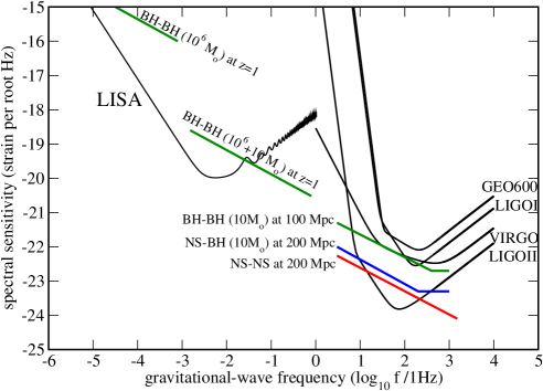
Figure 4: Estimated signal strengths for various inspiralling binaries relevant for ground- and space-based detectors.

Moreover, from

$$h_{xx}^{\mathrm{TT}}\approx-{2{\cal M}^{5/3}\Omega^{2/3}\over r}\cos 2\Omega(t-r)$$ (34)

we can estimate the effective amplitude of the binary signal:

$$h_{c}\approx\sqrt{ft}\ h\sim{M\over r}\left({R\over M}\right)^{1/4}$$ (35)

This shows that, even though the actual signal gets stronger, its detectability decreases as the orbit shrinks. Figure 4 compares our estimated gravitational-wave strain to the predicted noise-curves for various gravitational-wave detectors. Essentially, one would expect that

• Advanced LIGO may observe several binary systems per year.

• The space-based LISA detector may suffer an “embarrassment of riches”, with a large number of known galactic binaries leading to detectable signals (most likely generating to a “binary noise” which will be difficult to filter out).

To predict the rate at which the binary orbit shrinks as a result of gravitational-wave emission we need to estimate to total energy of the system:

$$E={M_{1}v_{1}^{2}\over 2}+{M_{2}v_{2}^{2}\over 2}-{GM_{1}M_{2}\over R}=-{G\mu M\over 2R}=-G{{\cal M}^{5/3}\Omega^{2/3}\over 2}$$ (36)

From this we find that the period $P$ of the system changes as

$${\dot{P}\over P}=-{96\over 5}{G^{3}\over c^{5}}{\cal M}^{5/3}\Omega^{8/3}$$ (37)

For the binary pulsar 1913+16, the predicted change in orbital period agrees with the theoretical prediction to within 1%. This indirect proof that gravitational waves exist led to Hulse and Taylor being awarded the 1993 Nobel prize in physics.

Finally, note that that the chirp-mass $\cal M$ plays a key role in our various expressions. From

$${\dot{P}\over P}\sim{\cal M}^{5/3}\Omega^{8/3}\quad\mbox{ and }\quad h\sim{{\cal M}^{5/3}\Omega^{2/3}\over r}$$ (38)

we see that this is the only combination of the two masses that can be infered from the signal (at this level of approximation: higher order post-Newtonian corrections depend on the individual masses, the spins etcetera). Suppose that we detect both the change in the amplitude $h$ and the shift in the frequency. Then one can infer both the chirp mass and the distance to the source, and in effect coalescing binaries are standard candles which can be used to constrain cosmological parameters.

One often classifies gravitational-wave sources by the nature of the waves. This is convenient because the different classes require different approaches to the data-analysis problem;

• Chirps. As a binary system radiates gravitational waves and loses energy the two constituents spiral closer together. As the separation decreases the gravitational-wave amplitude increases, leading to a characteristic “chirp” signal.

• Bursts. Many scenarios lead to burst-like gravitational waves. A typical example would be black-hole oscillations excited during binary merger.

• Periodic. Systems where the gravitational-wave backreaction leads to a slow evolution (compared to the observation time) may radiate persistent waves with a virtually constant frequency. This would be the gravitational-wave analogue of the radio pulsars.

• Stochastic. A stochastic (non-thermal) background of gravitational waves is expected to have been generated following the Big Bang. One may also have to deal with stochastic gravitational-wave signals when the sources are too abundant for us to distinguish them as individuals.

3 High-frequency gravitational wave sources

Having introduced the key concepts required for a discussion of gravitational-wave physics we will now focus our attention on sources that radiate above a hundred Hz or so, i.e. which may at least in principle be detectable from the ground. As we will see there are strong motivations for constructing detectors which are sensitive up to (ideally) several kHz.

3.1 Radiation from binary systems

It is easy to understand why binary systems are considered the “best” sources of gravitational waves. They emit copious amounts or gravitational radiation, and for a given system we know quite accurately the amplitude and frequency of the gravitational waves in terms of the masses of the two bodies and their separation (see section 2.2).

The gravitational-wave signal from inspiraling binaries is approximatelly sinusoidal, see equation (34), with a frequency which is twice the orbital frequency of the binary. As the binary system evolves the orbit shrinks and the frequency increases in the characteristic chirp. Eventually, depending on the masses of the binaries, the frequency of the emitted gravitational waves will enter the bandwidth of the detector at the low-frequency end and will evolve quite fast towards higher frequencies. A system consisting of two neutron stars will be detectable by LIGO when the frequency of the gravitational waves is $\sim$10Hz until the final coalescence around 1 kHz. This process will last for about 15 min and the total number of observed cycles will be of the order of $10^{4}$, which leads to an enhancement of the detectability by a factor 100 (remember $h_{c}\sim\sqrt{n}h$). Binary neutron star systems and binary black hole systems with masses of the order of 50M_⊙ are the primary sources for LIGO. Given the anticipated sensitivity of LIGO, binary black hole systems are the most promising sources and could be detected as far as 200 Mpc away. For the present estimated sensitivity of LIGO the event rate is probably a few per year, but future improvements of detector sensitivity (the LIGO II phase) could lead to the detection of at least one event per month. Supermassive black hole systems of a few million solar masses are the primary source for LISA. These binary systems are rare, but due to the huge amount of energy released, they should be detectable from as far away as the boundaries of the observable universe. Finally, the recent discovery of the highly relativistic binary pulsar J0737-3039 Burgay03 enchanced considerably the expected coalescence event rate of NS-NS binaries Kalogera04 . The event rate for initial LIGO is in the best case 0.2 per year while advanced LIGO might be able to detect 20-1000 events per year.

3.2 Gravitational collapse

One of the most spectacular events in the Universe is the supernova (SN) collapse to create a neutron star (NS) or a black hole (BH). Core collapse is a very complicated event and a proper study demands a deep understanding of neutrino emission, amplification of the magnetic fields, angular momentum distribution, pulsar kicks, etc. There are many viable models for each of the above issues but it is still not possible to combine all of them together into a consistent explanation. Gravitational waves emanating from the very first moments of the core collapse might shed light on all the above problems and help us understand the details of this dramatic event. Gravitational collapse compresses matter to nuclear densities, and is responsible for the core bounce and the shock generation. The event proceeds extremely fast, lasting less than a second, and the dense fluid undergoes motions with relativistic speeds ($v/c\sim 0.2-0.4$). Even small deviations from spherical symmetry during this phase can generate significant amounts of gravitational waves. However, the size of these asymmetries is not known. From observations in the electromagnetic spectrum we know that stars more massive than $\sim 8M_{\odot}$ end their evolution in core collapse and that $\sim 90\%$ of them are stars with masses $\sim 8-20M_{\odot}$. During the collapse most of the material is ejected and if the progenitor star has a mass $M\lesssim 20M_{\odot}$ it leaves behind a neutron star. If $M\gtrsim 20M_{\odot}$ more than 10% falls back and pushes the proto-neutron-star (PNS) above the maximum NS mass leading to the formation of a black hole (type II collapsars). Finally, if the progenitor star has a mass $M\gtrsim 40M_{\odot}$ no supernova takes place. Instead, the star collapses directly to a BH (type I collapsars).

A significant amount of the ejected material can fall back, subsequently spinning up and reheating the nascent NS. Instabilities can be excited during such a process. If a BH was formed, its quasi-normal modes (QNM) can be excited for as long as the process lasts. “Collapsars” accrete material during the very first few seconds, at rates $\sim 1-2M_{\odot}$/sec. Later the accretion rate is reduced by an order of magnitude but still material is accreted for a few tenths of seconds. Typical frequencies of the emitted gravitational waves are in the range 1-3kHz for $\sim 3-10M_{\odot}$ BHs. If the disk around the central object has a mass $\sim 1M_{\odot}$ self-gravity becomes important and gravitational instabilities (spiral arms, bars) might develop and radiate gravitational waves. Toroidal configurations can be also formed around the collapsed object. Their instabilities and oscillations might be an interesting source of gravitational wavesZannoti . There is also the possibility that the collapsed material might fragment into clumps, which orbit for some cycles like a binary system (fragmentation instability Fryer2001 ).

The supernova event rate is 1-2 per century per galaxy Cappellaro and about 5-40% of them produce BHs through the fallback material FryerKalogera . Conservation of angular momentum suggests that the final objects should rotate close to the mass shedding limit, but this is still an open question, since there is limited knowledge of the initial rotation rate of the final compact object. Pulsar statistics suggest that the initial periods are probably considerably shorter than $20$ ms. This strong increase of rotation during the collapse has been observed in many numerical simulations (see e.g. FryerHeger ; DFM2002b ).

Core collapse as a potential source of gravitational waves has been studied for more than three decades (some of the most recent calculations can be found in Finn90 ; Zwerger1997 ; Rampp1998 ; Fryer2002 ; DFM2002b ; Ott2003 ; Kotake2003 ; Shibata03 ; Whisky ). All these numerical calculations show that signals from Galactic supernova ($d\sim 10$kpc) are detectable even with the initial LIGO/EGO sensitivity at frequencies $\lesssim$1kHz. Advanced interferometers can detect signals from distances of 1 Mpc but it will be difficult with the designed broadband sensitivity to resolve signals from the Virgo cluster ($\sim$15Mpc). The typical gravitational wave amplitude from the 2D numerical simulations DFM2002b ; Ott2003 for an observer located on the equatorial plane of the source is

$$h\approx 9\times 10^{-21}\varepsilon\left({10{\rm kpc}\over d}\right)$$ (39)

where $\varepsilon\sim 1$ is the normalized gravitational wave amplitude. The total energy radiated in gravitational waves during the collapse is $\lesssim 10^{-6}-10^{-8}M_{\odot}c^{2}$. However, these numerical estimates are not yet conclusive, as important aspects such as 3D hydrodynamics combined with proper spacetime evolution have been neglected. The influence of the magnetic fields have been ignored in most calculations. The proper treatment of these issues might not change the above estimates by orders of magnitude but it will provide a conclusive answer. There are also issues that need to be understood such as the pulsar kicks (velocities even higher than 1000 km/s) which suggest that in a fraction of newly-born NSs (and BHs) the process may be strongly asymmetric Caraveo93 ; Burrows1996 ; Muller97 ; Spruit98 ; Loveridge . Also, the polarization of the light spectra in supernovae indicates significant asymmetries Wheeler1999 . Better treatment of the microphysics and construction of accurate progenitor models for the angular momentum distributions are needed. All these issues are under investigation by many groups.

Accretion Incuded Collapse (AIC) is also a possible source of high frequency gravitational waves. AIC takes place when a white dwarf (WD) exceeds the Chandrasekhar limit due to accretion of material and begins to collapse. The cooling via neutrino emission does not reduce the heating significantly and the collapsing WDs reach appropriate temperatures for ignition of nuclear burning (Type Ia supernova). Estimates suggest that about $0.1M_{\odot}$ material is ejected. Since the WD is pushed over the Chandrasekhar limit due to accretion, it will rotate fast enough to allow various types of instabilities Lindblom01 . The galactic rate of accretion induced collapse is about $10^{-5}$/yr which means that AIC are about 1000 times rarer than core collapse SN.

3.3 Rotational instabilities

Newly born neutron stars are expected to rotate rapidly enough to be subject to rotation induced instabilities. These instabilities arise from non-axisymmetric perturbations having angular dependence $e^{im\varphi}$. Early Newtonian estimates have shown that a dynamical bar-mode ($m=2$) instability is excited if the ratio $\beta=T/W$ of the rotational kinetic energy $T$ to the gravitational binding energy $W$ is larger than $\beta_{\rm dyn}=0.27$. The instability develops on a dynamical time scale (the time that a sound wave needs to travel across the star) which is about one rotation period, and may last from 1 to 100 rotations depending on the degree of differential rotation in the PNS. Another class of instabilities are those driven by dissipative effects such as fluid viscosity or gravitational radiation. Their growth time is much longer (many rotational periods) but they can be excited for significantly lower rotational rates, $\beta\gtrsim 0.14$ in the case of the fundamental modes of oscillation of the star.

3.4 Bar-mode instability

The dynamical bar-mode instability can be excited in a hot PNS, a few milliseconds after the core-bounce, given a sufficiently large $\beta$. It might also be excited a few tenths of seconds later, when the NS cools enough due to neutrino emission and contracts still further ($\beta\sim 1/R$). The amplitude of the emitted gravitational waves can be estimated as $h\sim MR^{2}\Omega^{2}/d$, where $M$ is the mass of the body, $R$ its size, $\Omega$ the rotational rate and $d$ the distance from Earth. This leads to an estimate of the gravitational wave amplitude

$$h\approx 9\times 10^{-23}\left({\epsilon\over 0.2}\right)\left({f\over 3{\rm kHz}}\right)^{2}\left({15{\rm Mpc}\over d}\right)M_{1.4}R_{10}^{2}.$$ (40)

where $\epsilon$ measures the ellipticity of the bar. Note that the gravitational wave frequency $f$ is twice the rotational frequency $\Omega$. Such a signal is detectable only from sources in our galaxy or the nearby ones (our Local Group). If the sensitivity of the detectors is improved in the kHz region, then signals from the Virgo cluster may be detectable. If the bar persists for many ($\sim$ 10-100) rotation periods, then even signals from distances considerably larger than the Virgo cluster could be detectable, cf. Figure 5. The event rate is of the same order as the SN rate (a few events per century per galaxy): this means that given the appropriate sensitivity at frequencies between 1-3kHz we might be able to observe a few events per year. The bar-mode instability may also be excited during the merger of NS-NS, BH-NS, BH-WD and even in type II collapsars (see discussion in Kobayasi2003 ).

In general, the above estimates rely on Newtonian hydrodynamics calculations; GR enhances the onset of the instability slightly, $\beta_{\rm dyn}\sim 0.24$ SBS2000 and $\beta_{\rm dyn}$ may be even lower for large values of the compactness (larger $M/R$). The bar-mode instability may be excited for significantly smaller $\beta$ if centrifugal forces produce a peak in the density off the sources rotational centerCentrella2001 . Rotating stars with a high degree of differential rotation are also dynamically unstable for significantly lower $\beta_{\rm dyn}\gtrsim 0.01$ Shibata2002 ; Shibata2003 . In this scenario the unstable neutron star settles down to a non-axisymmetric quasistationary state which is a strong emitter of quasi-periodic gravitational waves

$$h_{\rm eff}\approx 3\times 10^{-22}\left({R_{\rm eq}\over 30{\rm km}}\right)\left({f\over 800{\rm Hz}}\right)^{1/2}\left({100{\rm Mpc}\over d}\right)M_{1.4}^{1/2}.$$ (41)

The bar-mode instability of differentially rotating neutron stars could be an excellent source of gravitational waves provided that the dissipation of non-axisymmetric perturbations by viscosity and magnetic fields is negligible. That this is the case is far from clear. Magnetic fields might actually enforce the uniform rotation of the star on a dynamical timescale and the persistent non-axisymmetric structure might not have time to develop at all.

Numerical simulations have shown that the $m=1$ one-armed spiral mode might become dynamically unstable for considerably lower rotational rates Centrella2001 ; SBM2003 . This $m=1$ instability depends critically on the softness of the equation of state (EoS) and the degree of differential rotation.

3.5 CFS instability, f- and r-modes

After the initial bounce, neutron stars may maintain a considerable amount of deformation. They settle down to an axisymmetic configuration mainly due to emission of gravitational waves, viscosity and magnetic fields. During this phase QNMs are excited. Technically speaking, an oscillating non-rotating star has equal values $\pm|\sigma|$ (the frequency of a mode) for the forward and backward propagating modes (corresponding to $m=\pm|m|$). Rotation changes the mode frequency by an amount $\delta\sigma\sim m\Omega$ and both the prograde and retrograde modes will be dragged forward by the stellar rotation. If the star spins sufficiently fast, the originally retrograde mode will appear to be moving forwards in the inertial frame (according to an observer at infinity), but still backwards in the rotating frame (for an observer rotating with the star). Thus, an inertial observer sees gravitational waves with positive angular momentum emitted by the retrograde mode, but since the perturbed fluid rotates slower than it would in absence of the perturbation, the angular momentum of the mode itself is negative. The emission of gravitational waves consequently makes the angular momentum of the mode increasingly negative leading to an instability. From the above, one can easily conclude that a mode will be unstable if it is retrograde in the rotating frame and prograde for a distant observer measuring a mode frequency $\sigma-m\Omega$ i.e. the criterion will be $\sigma(\sigma-m\Omega)<0$.

This class of frame-dragging instabilities is usually referred to as Chandra-sekhar–Friedman–Schutz (CFS) Chandra70 ; FS78 instabilities. For the high frequency ($f$ and $p$) modes the instability is possible only for large values of $\Omega$ or for quite large $m$. In general, for every mode there will always be a specific value of $\Omega$ for which the mode will become unstable, although only modes with $|m|<5$ have an astrophysically significant growth time. The CFS mechanism is not only active for fluid modes but also for the spacetime or the so-called w-modesKRA2002 . It is easy to see that the CFS mechanism is not unique to gravitational radiation: any radiative mechanism will have the same effect.

In GR, the f-mode ($l=m=2$) becomes unstable for $\beta\approx 0.06-0.08$ SF1998 . If the star has significant differential rotation the instability is excited for somewhat higher values of $\beta$ (see e.g. Yoshida ; Stergioulas2003 ). The $f$-mode instability is an excellent source of gravitational waves. After the brief dynamical phase, the PNS becomes unstable and the instability deforms the star into a non-axisymmetric configuration via the $l=2$ bar mode. Since the star loses angular momentum it spins down, and the gravitational wave frequency sweeps from 1 kHz down to about 100 Hz LaiShapiro95 . If properly modelled such a signal can be detected from a distance of 100 Mpc (if the mode grows to a large nonlinear amplitude).

Rotation not only shifts the frequencies of the various modes; it also gives rise to the Coriolis force, and an associated new family of rotational or inertial modes. Inertial modes are primarily velocity perturbations. Of special interest is the quadrupole inertial mode ($r$-mode) with $l=m=2$. The frequency of the $r$-mode in the rotating frame of reference is $\sigma=2\Omega/3$. Using the CFS criterion for stability we can easily show that the $r$-mode is unstable for any rotation rate of the star. For temperatures between $10^{7}-10^{9}$K and rotation rates larger than 5-10% of the Kepler limit, the growth time of the unstable mode is much shorter than the damping times due to bulk and shear viscosity. The mode grows until it saturates due to non-linear effects LOM98 ; Owen98 ; AKS99 . The strength of the emitted gravitational waves depends on the saturation amplitude $\alpha$. Mode coupling might not allow the growth of the instability to amplitudes larger than $\alpha\approx 10^{-2}-10^{-3}$ Arras2002 . The existence of a crust Bildsten99 ; LOU2000 or of hyperons in the core LO2002 and strong magnetic fields Rezzolla2000 , affect the efficiency of the instability (for extended reviews see AK2001 ; Nils2003 ). For newly-born neutron stars the amplitude of gravitational waves might not be such that the signals will be detectable only from the local group of galaxies ($d<1$Mpc)

$$h(t)\approx 10^{-21}\alpha\left({\Omega\over 1{\rm kHz}}\right)\left({100{\rm kpc}\over d}\right)$$ (42)

see Figure 5.

If the compact object is a strange star, then the r-mode instability will not reach high amplitudes ($\alpha\sim 10^{-3}-10^{-4}$) but it will persist for a few hundred years and in this case there might be up to ten unstable stars per galaxy radiating gravitational waves at any time AJK2002 . Integrating data for a few weeks can then lead to an effective amplitude $h_{\rm eff}\sim 10^{-21}$ for galactic signals at frequencies $\sim 700-1000$Hz. The frequency of the signal changes only slightly on a timescale of a few months, so the radiation is practically monochromatic.

Old accreting neutron stars, radiating gravitational waves due to the $r$-mode instability, at frequencies 400-700Hz, are probably a better source AKS1999 ; AJKS2000 ; Heyl ; Wagoner . Still, the efficiency and the actual duration of the process depends on the saturation amplitude $\alpha$. If the accreting compact object is a strange star or has a hyperon core then it might be a persistent source which radiates gravitational waves for as long as accretion lasts AJK2002 ; Reisenegger .

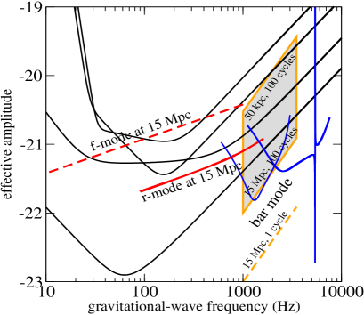
Figure 5: The estimated strength of gravitational waves from the dynamical bar-mode instability and the CFS instability of the f- and r-modes. The estimates are compared to the predicted noise of the various interferometers and also the possible noise curve for a dual cylinder detector.

3.6 Oscillations of black holes and neutron stars

Black-hole ringing. The merger of two neutron stars or black holes or the collapse of a supermassive star (collapsar of type I or II) will produces a black hole. The newly formed black hole will ring, emitting a characteristic signal until it settles down to the stationary Kerr state. This characteristic signal, the so-called quasi-normal mode oscillation, will be a unique probe of the black hole’s existence. Although the ringing phase does not last very long (a few tenths of a ms), the ringing due to the excitation by the fallback material might last for secsAraya03 ; Nagar04 . The frequency and damping time of the black-hole ringing for the $l=m=2$ oscillation mode can be estimated via the relations Echeverria

$$\sigma \approx 3.2{\rm kHz}\ M_{10}^{-1}\left[1-0.63(1-a/M)^{3/10}\right]$$ (43)

$$Q = \pi\sigma\tau\approx 2\left(1-a\right)^{-9/20}$$ (44)

These relations together with similar ones either for the 2nd QNM or the $l=2$, $m=0,\pm 1$ can uniquely determine the mass $M$ and angular momentum $a$ of the BH if the frequency and the damping time of the signal have been accurately extracted Finn ; Dryer . The amplitude of the ring-down waves depends on the BH’s initial distortion. If the excitation of the BH is due to infalling material then the energy is roughly $\Delta E\gtrsim\epsilon\mu c^{2}(\mu/M)$ where $\epsilon\gtrsim 0.01$ Davis1971 . This leads to an effective gravitational wave amplitude

$$h_{\rm eff}\approx 2\times 10^{-21}\left({\epsilon\over 0.01}\right)\left({10{\rm Mpc}\over d}\right)\left({\mu\over M_{\odot}}\right)$$ (45)

This approximate result has been verified by more detailed full non-linear simulations Anninos

Neutron star ringing. If the collapse leaves behind a compact star, various types of oscillation modes might be excited which can help us estimate parameters of the star such as radius, mass, rotation rate and EoSAK1998 ; KAA2001 ; AC2001 . This gravitational wave asteroseismology is a unique way to find the radius and the EoS of compact stars. One can derive approximate formulas in order to connect the observable frequencies and damping times of the various stellar modes to the stellar parameters. For example, for the fundamental oscillation ($l=2$) mode ($f$-mode) of non-rotating stars we get AK1998

$$\sigma({\rm kHz}) \approx 0.8+1.6M_{1.4}^{1/2}R_{10}^{-3/2}+\delta_{1}m{\bar{\Omega}}$$ (46)

$$\tau^{-1}({\rm secs}^{-1}) \approx M_{1.4}^{3}R_{10}^{-4}\left(22.9-14.7M_{1.4}R_{10}^{-1}\right)+\delta_{2}m{\bar{\Omega}}$$ (47)

where ${\bar{\Omega}}$ is the normalized rotation frequency of the star, and $\delta_{1}$ and $\delta_{2}$ are constants estimated by sampling data from various EoS. The typical frequencies of the NS modes are higher than 1 kHz. On the other hand, 2D simulations of rotating core-collapse have shown that if a rapidly rotating NS is created, then the dominant mode is the quasi-radial mode (“$l=0$”), radiating through its $l=2$ piece at frequencies $\sim$ 800Hz-1kHz DFM2002b . Since each type of mode is sensitive to the physical conditions where the amplitude of the mode eigenfunction is greatest, the more information we get from the various classes of modes the better we will understand the details of the star.

Concluding, we should mention that the tidal disruption of a NS by a BH Vallisneri or the merging of two NSs Rasio may give valuable information for the radius and the EoS if we can detect the signal at frequencies higher than 1 kHz.

This work has been supported by the EU Programme ’Improving the Human Research Potential and the Socio-Economic Knowledge Base’ (Research Training Network Contract HPRN-CT-2000-00137). KK acknowledges support throught the Center of Gravitational Wave Physics, which is funded by the NSF number cooperative agreement PHY 01-14375.

References

- (1) C. Cutler, K.S. Thorne: in proceedings of GR16 (Durban South Africa, 2001), gr-qc/0204090
- (2) R. Schnabel, J. Harms, K.A Strain, K. Danzmann: Class. Quantum Grav. 21, S1155 (2004)
- (3) M. Bonaldi, M. Cerdonio, L. Conti, G.A. Prodi, L. Taffarello, J.P. Zendri: Class. Quantum Grav. 21, S1155 (2004)
- (4) M. Burgay, N. D’Amico, A. Possenti, R.N. Manchester, A.G. Lyne, B.C. Joshi, M.A. McLaughlin, M. Kramer, J.M. Sarkissian, F. Camilo, V. Kalogera, C. Kim, D.R. Lorimer: Nature, 426, 531 (2003)
- (5) V. Kalogera, C. Kim, D.R. Lorimer, M. Burgay, N. D’Amico, A. Possenti, R.N. Manchester, A.G. Lyne, B.C. Joshi, M.A. McLaughlin, M. Kramer, J.M. Sarkissian, F. Camilo: Astrophys.J. 601, L179 (2004)
- (6) E. Cappellaro, M. Turatto, D.Yu. Tsvetov, O.S. Bartunov, C. Pollas, R. Evans and M. Hamuy: A&A 351, 459 (1999)
- (7) O. Zanotti, L. Rezzolla, J. A. Font: M.N.R.A.S., 341 832 (2003)
- (8) C.L. Fryer, S.E. Woosley, A. Heger: Astrophys. J. 550, 372 (2001)
- (9) C.L. Fryer, V. Kalogera: Astrophys. J. 554, 548 (2001)
- (10) C.L. Fryer, A. Heger: Astrophys. J. 541 1033 (2000)
- (11) H. Dimmelmeier, J.A. Font, E. Muller: A& A 393, 523 (2002)
- (12) S.L. Finn, C.R. Evans: Astrophys. J, 351, 588 (1990)
- (13) T. Zwerger, E. Müller: A & A 320, 209 (1997)
- (14) M. Rampp, E. Müller, M. Ruffert: A& A 332, 969 (1998)
- (15) C.L. Fryer, D.E. Holz, S.A. Hudges: Astrophys. J. 565, 430 (2002)
- (16) C.D. Ott, A. Burrows, E. Livne, R. Walder: Astrophys. J. 600, 834 (2004)
- (17) K. Kotake, S. Yamada, K. Sato K: Phys. Rev. D 68, 044023 (2003)
- (18) M. Shibata: Astrophys. J. 595, 992 (2003)
- (19) L. Baiotti, I. Hawke, P. . Montero, F. Löffler, L. Rezzolla, N. Stergioulas, J.A. Font, E. Seidel, gr-qc/0403029
- (20) P.A. Caraveo: Astrophys. J. 415, L111 (1993)
- (21) A. Burrows, J. Hayes: Phys. Rev. Lett. 76, 1037 (1996)
- (22) E. Müller, H.-Th. Janka: A& A 317, 140 (1997)
- (23) H.C. Spruit, E.S. Phinney: Nature 393, 139 (1998)
- (24) L.C. Loveridge: Phys. Rev. D 69,024008 (2004)
- (25) P. Hoeflich, A. Khokhlov, L. Wang, J.C. Wheeler, D. Baade: IAU Symposium 212 on Massive Stars, D. Reidel Conf. Series, ed. E. van den Hucht, astro-ph/0207272
- (26) Y.T Liu, L. Lindblom: M.N.R.A.S. 324, 1063 (2001)
- (27) S. Kobayasi, P. Meszaros: Astrophys. J. 589,861 (2003)
- (28) M. Shibata, T.W. Baumgarte, S.L. Shapiro: Astrophys. J. 542, 453 (2000)
- (29) J.M. Centrella, K.C.B. New, L.L. Lowe, J.D. Brown: Astrophys. J. Lett. 550 193 (2001)
- (30) M. Shibata, S. Karino, Y. Eriguchi: M.N.R.A.S. 334, L27 (2002)
- (31) M. Shibata, S. Karino, Y. Eriguchi: M.N.R.A.S. 343, 619 (2003)
- (32) M. Saijo, T.W. Baumgarte, S.L. Shapiro: Astrophys. J. 595, 352 (2002)
- (33) K.D. Kokkotas, J. Ruoff, N. Andersson: gr-qc/0212419
- (34) S. Chandrasekhar: Phys. Rev. Lett. 24, 611 (1970)
- (35) J.L. Friedman, B.F. Schutz: Astroph. J. 222, 281 (1978)
- (36) N. Stergioulas, J.L. Friedman: Astrophys. J. 492, 301 (1998)
- (37) S. Yoshida, L. Rezzolla, S. Karino, Y. Eriguchi: Astrophys. J. Lett. 568, 41 (2002)
- (38) N. Stergioulas: Living Reviews in Relativity 6 3 (2003)
- (39) D. Lai, S.L. Shapiro: Astrophys. J. 442, 259 (1995)
- (40) L. Lindblom, B.J. Owen, S.M. Morsink, Phys. Rev. Lett. 80 4843 (1998)
- (41) B. Owen, L. Lindblom, C. Cutler, B.F. Schutz, A. Vecchio, N. Andersson: Phys. Rev. D 58, 084020 (1998)
- (42) N. Andersson, K.D. Kokkotas, B.F. Schutz: Astrophys. J. 510, 846 (1999)
- (43) L. Bildsten, G. Ushomirsky: Astrophys. J. 529, L33 (2000)
- (44) L. Lindblom, B.J. Owen, G. Ushomirsky: Phys. Rev. D 62, 084030 (2000)
- (45) A.K. Schenk, P. Arras, E.E. Flanagan, S.A. Teukolsky, I. Wasserman: Phys. Rev. D 65, 024001 (2002)
- (46) L. Rezzolla, F.K. Lamb, S.L. Shapiro: Astrophys. J. 531, L139 (2000)
- (47) L. Lindblom, B. Owen: Phys. Rev. D 65, 063006 (2002)
- (48) N. Andersson and K. D. Kokkotas: I.J.M.P. D10,381 (2001)
- (49) N. Andersson: Class. Quantum Grav. 20 R105 (2003)
- (50) N. Andersson, K.D. Kokkotas, N. Stergioulas: Astrophys. J. 307, 314 (1999)
- (51) N. Andersson, D.I. Jones, K.D. Kokkotas, N. Stergioulas: Astrophys. J. Lett. 534 L75 (2000)
- (52) J. Heyl: Astrophys. J. Lett. 574 L57 (2002)
- (53) R.V. Wagoner: Astrophys. J. Lett. 578 L63 (2002)
- (54) N. Andersson, D.I. Jones, K.D. Kokkotas: M.N.R.A.S. 337 1224 (2002)
- (55) A. Reisenegger, A. Bonacic: Phys. Rev. Lett. 91, 201103 (2003)
- (56) R.A. Araya-Góchez astro-ph/0311001
- (57) A. Nagar, G. Diaz, J.A. Pons, J.A.Font gr-qc/0403077)
- (58) E. Echeverria: Phys. Rev. D 40 3194 (1988)
- (59) L.S. Finn: Phys. Rev. D 8 3308 (1992)
- (60) O. Dryer, B. Kelly, B. Krishnan, L.S. Finn, D. Garrison, R. Lopez-Aleman: Class. Quantum Grav. 21, 787 (2004)
- (61) M. Davis, R. Ruffini, W.H. Press, R.H. Price: Phys. Rev. Lett.27, 1466 (1971)
- (62) P. Anninos, R.H. Price, J. Pullin, E. Seidel, W.-M. Suen: Phys. Rev. D 52, 4462 (1995)
- (63) N. Andersson, K.D. Kokkotas: M.N.R.A.S. 299, 1059 (1998)
- (64) K.D. Kokkotas, T. Apostolatos, N. Andersson: M.N.R.A.S. 320 307 (2001)
- (65) N. Andersson, G.L. Comer: Phys. Rev. Lett.87, 241101 (2001)
- (66) M. Vallisneri: Phys. Rev. Lett. 84 3519 (2000)
- (67) J.A. Faber, P. Grandclement, F.A. Rasio, K. Taniguchi: Phys. Rev. Lett. 89 231102 (2002)