Long term study of the seismic environment at LIGO

Abstract

The LIGO experiment aims to detect and study gravitational waves using ground based laser interferometry. A critical factor to the performance of the interferometers, and a major consideration in the design of possible future upgrades, is isolation of the interferometer optics from seismic noise. We present the results of a detailed program of measurements of the seismic environment surrounding the LIGO interferometers. We describe the experimental configuration used to collect the data, which was acquired over a 613 day period. The measurements focused on the frequency range 0.1–10 Hz, in which the secondary microseismic peak and noise due to human activity in the vicinity of the detectors was found to be particularly critical to interferometer performance. We compare the statistical distribution of the data sets from the two interferometer sites, construct amplitude spectral densities of seismic noise amplitude fluctuations with periods of up to 3 months, and analyze the data for any long term trends in the amplitude of seismic noise in this critical frequency range.

1 Introduction

The LIGO laboratory has constructed three long-baseline laser interferometers whose object is the direct detection and subsequent study of gravitational radiation from astrophysical sources [1].

The LIGO interferometers are located at two sites in the U.S.A., two interferometers of arm lengths 2km and 4km at the Department of Energy Hanford Site near Hanford, Washington, and a single 4km arm length interferometer located in Livingston Parish, Louisiana. We refer to these two observatories subsequently as Hanford and Livingston. Figure 1 shows greatly simplified schematics of the interferometers.

Figure 1: A simplified schematic diagram showing the layout of the LIGO interferometers, and the approximate positions of the seismometers at the sites. Note that the cartesian axes define the three components of velocity relative to the interferometer arms. The direction of true north with respect to the interferometer arms for each site is indicated by the arrow labelled with N. By true north, we mean the direction parallel to the line of constant longitude passing through the corner station building of the LIGO site in question.

The LIGO detectors have been described in detail elsewhere [2]. Each detector consists of a Michelson interferometer with the two interferometer arms at right angles. Each arm consists of a 2 or 4 kilometer long Fabry-Perot resonant cavity. A laser beam is split into two components which coherently excite one resonant mode of each Fabry-Perot cavity. At resonance, where the cavity length $L$ is a multiple of half the laser wavelength $\lambda$, there is no phase shift between the beam incident on the near-end mirror of each cavity and the beam passing back towards the beam splitter from this same near-end mirror. For small deviations, $\Delta L$, from the resonant length, the phase shift is linear in $\Delta L$, as long as $\Delta L$ is small compared with $\mathrm{\Gamma_{L}=\lambda/2}\mathcal{F}$, where $\mathcal{F}$ is the finesse of the cavity. The LIGO interferometers have $\mathrm{\lambda=1.06~{}\mu m}$ and $\mathcal{F}\sim\mathrm{100}$, so $\mathrm{\Gamma_{L}\sim 5~{}nm}$. The detectors are designed to be sensitive to gravitational waves in the frequency range 50 Hz to 7 kHz.

Gravitational waves passing through the detectors would cause oscillatory perturbations in components of the metric. Consider first a simplified case, where the mirrors are freely floating, initially at fixed separation. Metric perturbations due to gravitational waves would cause the lengths of the two Fabry-Perot cavities in each interferometer to oscillate in antiphase. The amplitude of these oscillations from anticipated sources of gravitational waves are not known, but they are not expected to exceed $\Delta L/L=10^{-21}$. These oscillations would give rise to phase modulations of opposite signs in the light beams reflected from the near end of the two Fabry-Perot cavities back towards the beam splitter. By recombining these beams coherently at the beam splitter, we can measure the phase difference between them.

The response of the LIGO interferometers to gravitational waves is more complex than for the ideal case discussed above. Each mirror is supported against the Earth’s gravitational field. The reaction forces in this support system must be taken into account in calibrating the response of the LIGO interferometers to gravitational waves. Secondly, the LIGO interferometers utilize multiple feedback [3] and feedforward [4] control systems to minimize residual fluctuations in the lengths of the Fabry-Perot cavities. These control systems utilize electromagnetic actuators to exert forces on the LIGO mirrors to ensure that fluctuations in the arm lengths over the full interferometer bandwidth are sufficiently small to maintain linearity of the interferometer and readout electronics. The reaction of these control systems to gravitational waves must also be accounted for in calibration of the interferometers [3, 5].

There are more stringent constraints on the magnitude of interferometer arm length fluctuations than the $\mathrm{\pm 5~{}nm}$ required to ensure linearity in the response of the phase of the recombined signal at the beam splitter to length fluctuations. The interferometer optics are configured for a light intensity at the output photodetectors commensurate with high sensitivity to the small arm length fluctuations expected from gravitational waves. In this configuration, the photodetectors saturate for arm length fluctuations exceeding $\mathrm{1~{}pm}$. Furthermore, length fluctuations approaching this photodiode limit can result in excess noise in the gravitational wave band through bilinear coupling of laser amplitude and frequency noise into the interferometer. Fluctuations in the arm lengths are maintained to within these stringent limits by the servo controls described above.

A problem of great practical importance is lock acquisition, the process of bringing the mirrors from initially unconstrained motion on their supports, into a state where their residual motions are sufficiently small that the interferometer outputs are linear in changes in the arm lengths due to mirror displacements, and control systems are operating to maintain the resonant, high sensitivity state of the instrument [6]. We refer to loss of this sensitive instrument state as lock loss. When lock loss occurs, the interferometers are unuseable as gravitiational wave detectors until lock is re-acquired. The operation of the LIGO interferometers is largely concerned with maintaining lock for the largest possible percentage of the time.

A significant noise source for LIGO is seismic noise in the ground acting through the mirror supports and shaking the mirrors. In order to be sensitive to gravitational waves, the amplitude spectral density of noise fluctuations on the mirrors due to seismic noise over the 50–7000 Hz band should be significantly less than the expected signal amplitude of $\mathrm{\sim 10^{-18}~{}m}$. Secondly, the root mean square (r.m.s.) noise amplitude at each mirror over all frequencies should be significantly less than the $\mathrm{10^{-12}}$ m required to maintain lock.

As part of the LIGO scheme to meet these displacement noise requirements, each mirror support incorporates a multi-stage vibration isolation system. This system consists of a passive isolation stack [7] in series with a steel wire, single loop pendulum for which the mirror substrate forms the suspended mass. Both of these systems have natural resonant frequencies below the gravitational wave detection band. The 0.74 Hz pendulum resonance is damped using a local feedback control system. The passive isolation stack has several resonances between 1 and 15Hz, characterized by Qs of about 10–30.

In this paper we present results of a long term study of seismic noise at the two LIGO sites. The seismometer data recorded for this study reflect motion of the concrete slabs under the LIGO optic support structures. The results given here are not intended as a study of the seismic environment in the ground. To reflect this, we use the terms slab velocity and slab motion throughout this paper to denote the measured ground velocity on the concrete floors of the LIGO lab buildings, as opposed to measurements of ground velocity in a seismic vault that would be used by a geologist or geophysicist to study the geophysical properties of the local earth’s crust.

The data for this analysis were taken over a 613 day period between April 2nd 2001 and December 10th 2002. The analysis focuses on the frequency band 0.1–10 Hz. A central goal of this type of analysis is to study periodicities in the seismic environment at the sites and any correlations they might have with performance of the interferometers. It became clear during this analysis that slab noise in different parts of this frequency band was a good predictor of interferometer functionality. Furthermore, this analysis has demonstrated conclusively that the seismic environment at the Livingston interferometer is more challenging to ground-based gravitational wave interferometry than that at the Hanford site.

2 Locations and Environments of the LIGO Detectors

Herein follows a brief summary of the location of each of the two LIGO interferometer sites and environmental information about the two sites which is relevant to our analysis of the seismic data.

The Hanford interferometers are located on semi-arid shrub and grassland east of the Cascade mountains in Washington State on the Columbia Plateau, 370 km from the nearest point on the Pacific coast. The vertex latitude and longitude of the Hanford laboratory are $46^{\circ}27^{\prime}18.5^{\prime\prime}$ N, $119^{\circ}24^{\prime}27.6^{\prime\prime}$ W, and the x arm orientation is $324.0^{\circ}$ (NW). The plateau rests on a sequence of volcanic basalt flows called the Columbia River Basalt Group. These basalt formations are folded and faulted, and the resulting basins have filled with alluvial sedimentary deposits. The Hanford interferometers rest on the sediment of one of the larger basins known as the Pasco basin. The sediment depth exceeds the depth of the water table, which is approximately 120 m below the surface [9]. The nearest substantial population centers to the site are the cities of Richland, Pasco, and Kennewick, which in 2002 had a combined population of 124,000 [10]. The three cities are 20, 33, and 35 kilometers from the LIGO site. The LIGO Hanford laboratory is also located 15 km from sites 200E and 200W, facilities run by the Department of Energy which are currently carrying out extensive environmental cleanup operations which involve use of heavy earth moving machinery. The Hanford site climatology is described in detail in [8]. The average annual rainfall 18 cm. During the summer months, the site is subject to strong day-night air temperature fluctuations. In July and August the maximum daytime and minimum nighttime temperatures are typically $\mathrm{32~{}^{\circ}C}$ and $\mathrm{16~{}^{\circ}C}$. Strong wind gusts, which can cause increased motion of the concrete slabs supporting the LIGO instruments, are observed. Peak wind gusts speeds in a one month period are typically between $\mathrm{29~{}m/s}$ and $\mathrm{36~{}m/s}$. Gusts above $\mathrm{18~{}m/s}$ are more frequent in the months January to April.

The Livingston site is located in managed pine forest and more general forested land in southeastern Louisiana, 54 km from the nearest point on Lake Ponchatrain, and 130 km from the nearest point on the Gulf of Mexico. The vertex latitude and longitude of the Livingston laboratory are $30^{\circ}33^{\prime}46.4^{\prime\prime}$ N, $90^{\circ}46^{\prime}27.3^{\prime\prime}$ W, and the x arm orientation is $252.3^{\circ}$ (WSW). The geology local to the site consists of silt, sand, and mud alluvium, deposited by the Mississippi river. The bulk of this material was deposited before 2 million years ago when the Gulf coast moved south to approximately its present position along with the bulk of new Mississippi silt deposits. The water table is less than a meter below the ground, so the interferometer buildings rest on earth banking, consisting of the local silt and sand, raised several meters above the natural ground level. The Livingston interferometer corner station is 7 km from the center of the town of Livingston, which in 2000 had a population of 1,342 [10]. Climatological data is available from [12]. The average annual rainfall in Livingston Parish is 152 cm. Violent rain and windstorms occur frequently, especially during August and September. Winter minimum and summer maximum temperatures are around $\mathrm{0~{}^{\circ}C}$ and $\mathrm{33~{}^{\circ}C}$ respectively. A particularly important environmental factor for seismic noise is the use of local land for timber harvesting. The heavy machinery used for logging adjacent to the site is a significant source of seismic noise for the interferometer. A second important environmental factor affecting seismic noise at the instruments is the passage of cargo trains along the railroad track 7km to the south of the interferometer corner station. Large trains that run past the site twice every evening currently disrupt the operation of the interferometer for around 40 minutes out of every day. For this paper we do not attempt to separate data from the Livingston site into that taken during the passage of trains and that without. We present instead a broad statistical overview of the seismic environment over a long time period.

Figure 2: Data flow from ground to blrms data file. The filters used to band limit the decimated data are autoregressive, meaning that they use previous values of output data from the filter as well as input data to determine each new output data value. These filters have the useful property that the reciprocal of the lower pass band edge frequency of the filter can be longer than the time duration of the data segment used to calculate the filtered data output. The sampling rate in the decimated data is chosen to be over twice the upper pass band edge frequency of the filter. For example, the 0.1–0.3 Hz filter uses input data decimated to a sampling rate of 1 Hz, and 8 samples each of input and previous output data are used to determine each new filtered data point. For this example, only 8 seconds worth of data is needed to implement the lower band edge at a frequency of 1/10 Hz.

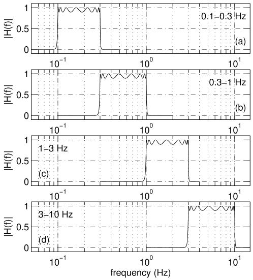
Figure 3: Magnitudes of the transfer functions of the four time domain bandpass filters applied to the seismometer data. The vertical axis is the ratio of the amplitudes of the filter output to the filter input for a test sinusoidal signal applied to the filter input, in the frequency range indicated on the horizontal axis. Each filter is a 16th order elliptic type having 1dB of passband ripple and 80dB of stopband attenuation.

3 Data Acquisition

Data for this analysis were acquired using seismometers and acquisition hardware installed as part of the LIGO data acquisition system. Figure 1 shows the approximate locations of the 8 seismometers at the two LIGO sites used in this experiment. The seismometers are Guralp CMG-40T three-axis types [14], whose outputs are proportional to the three cartesian components of slab velocity for disturbances in the frequency range 0.1–10 Hz. Figure 2 is a schematic of the data acquisition and the processing applied to the data. The voltage output of each seismometer channel is passed through an antialiasing lowpass filter with a knee frequency of 900 Hz, and is then digitized by an ICS-110B 16 bit A.D.C. [16] at a sampling rate of 2048Hz. The A.D.C. is housed in a V.M.E. crate controlled by an 800MHz pentium-based CPU running VxWorks [17], a real time operating system. A time stamp is added to the data using a brandywine GPS receiver [15] installed in the V.M.E. crate.

The data acquired by the real time system are sent via fiber to a shared memory partition on the backplane of a sun microsystems server which provides an online data analysis environment [13] under UNIX. Software running in this environment performs the analysis in real time. The data are decimated to successively lower sampling rates, and passed through a bank of time-domain, bandpass filters. The filter frequency bands are 0.1–0.3 Hz, 0.3–1 Hz, 1–3 Hz, and 3–10 Hz. Figure 3 shows the magitudes of the filter transfer functions for the four bands. The sum of the squares of the filtered data bins is measured once a second, and 60 of these measurements taken in successive seconds are used to compute the r.m.s. slab velocity at 1 minute intervals. The r.m.s. data are written to disk.

4 Results

4.1 The 0.1–0.3 Hz Frequency Band

With the exception of short time periods during earthquakes, seismic noise in this band is dominated by ‘secondary microseisms’ [18]. They consist of travelling surface waves in the earth’s crust. The sources of these waves are complex, but they are thought to originate in the pressure from counter-propagating ocean waves against the ocean bottom near the coasts of the land masses, as well as from more distant deep-ocean storms. Their frequency content peaks in the range 0.05 - 0.5 Hz, but the position and shape of the peak is highly non-stationary within this range. Large amplitude secondary microseisms are often observed during costal storms.

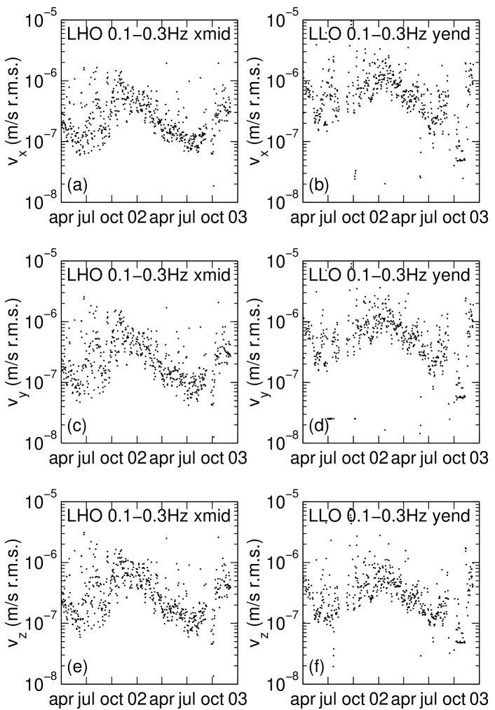
Figure 4: Time series of the three cartesian components of ground velocity in $\mathrm{ms^{-1}}$ at the $x$ midstation at Hanford (left column) and the $y$ endstation at Livingston (right column). The $x$ and $y$ components are parallel to the ground, the $z$ component is vertical. Each point represents the r.m.s. in the frequency band 0.1–0.3 Hz over one day. The independent variable ticks represent midnight on the first of every third month, with the beginnings of years labelled by the year number. These ticks are not evenly spaced because successive three month intervals do not all contain the same number of days.

Figure 5: A cumulative histogram of r.m.s. velocity in the 0.1–0.3 Hz band. The ordinate of the curve is the fraction of minute-duration data segments having r.m.s. velocity greater than the abscissa, The plot on the left gives results for a horizontal ($x$) and the vertical ($z$) components measured by the Livingston corner station seismometers. The right hand plot gives results for a horizontal ($x$) and the vertical ($z$) componenets measured by the Hanford corner station seismometer. The number of points in the histograms is 704150 (710212) for the Livingston horizontal (vertical) axis histograms and 674286 (685362) for the Hanford horizontal (vertical) axis histograms.

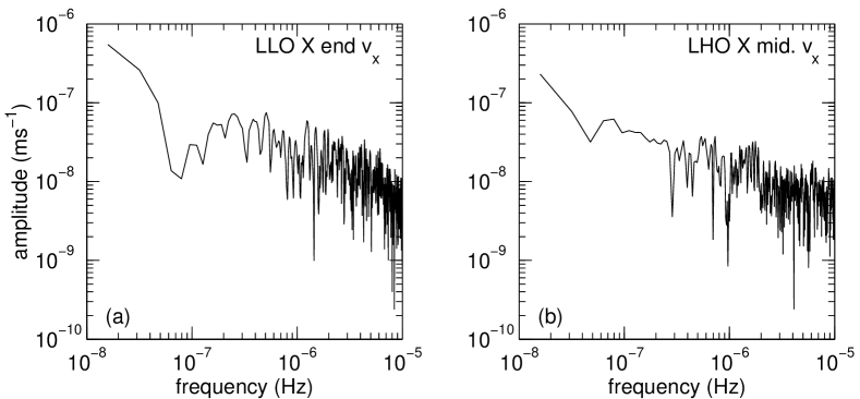
Figure 6: Amplitude spectra of the time series output of the 0.1–0.3 Hz filtered r.m.s. measurements from the $x$ axes horizontal output of the Livingston X endstation and Hanford X midstation seismometers.

Figure 4 shows r.m.s. in the 0.1 - 0.3 Hz band over 613 days. All the data exhibit a marked annual modulation, with the peaks of the modulation in the winter months and the troughs in the summer. Figure 5 shows cumulative histograms of all the velocity measurements taken over the 613 day period. Since the two horizontal velocity components are similar, and we do not see significant differences between the results for different seismometers at the same LIGO site in this band, results are given for a single horizontal component and vertical velocity for each site. Table 1 shows summary data for the 0.1–0.3 Hz band from each axis of 3 seismometers from each site. The percentile values represent the velocities below which the given percentage of readings of the r.m.s. came over the 613 days of measurements.

Seismometers located in different buildings, but at the same site, gave similar results in this frequency band. This is as expected, since the microseismic wave amplitudes should not differ significantly over a distance of order 4km. The results in table 1, and Figure 5 indicate that the Hanford site is noisier than the Livingston site in this band by a factor of 2-3 in the horizontal components. In the vertical components, the ratio is different at the 50th percentile level than at the 90th or 95th percentile level. The 50th percentile noise levels are a factor of 1-2 higher at Livingston than at Hanford. At the 90th and 95th percentile levels, a long tail in the cumulative statistics from Hanford implies that 5 to 10 percent of the time the Hanford site is at least 80% as noisy as the Livingston site.

It is interesting to note that the vertical components of seismic noise at Livingston are less than the horizontal components by almost a factor of 2, at all percentile levels, where at Hanford the vertical components equal or slightly exceed the horizontal components. Simplified theoretical models [18] treat the Earth’s crust as an isotropic half space of uniform composition, and contain two classes of traveling surface waves. Rayleigh waves are elliptically polarized in the plane whose normal is perpendicular to the wave vector and parallel to the Earth’s surface, and therefore produce both horizontal and vertical slab motion. Love waves are linearly polarized parallel to the plane of the Earth’s surface and perpendicular to the direction of propagation of the wave. Therefore Love waves produce only horizontal motion. Assuming that the site slab motion can be decomposed into two components, due to Rayleigh waves and Love waves, we conclude that differences in the sources and the geology through which the waves have travelled to reach the sites cause the ellipticity of the Rayleigh waves, the relative intensities of Rayleigh to Love waves, or a combination of these factors, to differ between the sites. The data do not allow us to make a direct comparison between the relative amplitudes of the Rayleigh and Love wave components at the two sites.

Figure 6 shows the amplitude spectral densities of the time series of measurements of r.m.s. slab velocity in the $x$ axes of the Livingston X end station and Hanford X mid station seismometers. The annual modulation apparent from the time series of figure 4 corresponds to a frequency of $\mathrm{3.17\times 10^{-8}}$ Hz. The resolution bandwidth of the power spectra are too low to resolve this peak from the zero frequency component, so accurate estimates of the amplitude of annual modulation of the microseism cannot be made without more data. There is no evidence for other, shorter periodicities. These amplitude spectra are typical of those from the full set of seismometers and seismometer axes. The amplitude spectral density of slab motion fluctuations drop as the inverse square root of frequency starting at $\mathrm{4\times 10^{-7}}$ Hz, corresponding to a 28 day period.

Table 1: Table of 50th, 90th, and 95th percentile measured r.m.s. ground velocities in three locations at each LIGO site, after applying a 0.1–0.3 Hz bandpass filter. In the percentage of one minute measurements given at the head of each column, the measured ground velocity in this band was less than the tabulated value.

• 0.1–0.3 Hz band
  site	building	axis	velocity percentile ($\mu\rm m\,s^{-1}$)
  			50%	90%	95%
  Livingston	Corner	$x$	0.49	1.2	1.7
  		$y$	0.53	1.3	1.7
  		$z$	0.27	0.69	0.91
  	X end	$x$	0.50	1.2	1.7
  		$y$	0.51	1.3	1.7
  		$z$	0.25	0.67	0.89
  	Y end	$x$	0.53	1.3	1.7
  		$y$	0.50	1.3	1.6
  		$z$	0.25	0.66	0.89
  Hanford	Corner	$x$	0.13	0.45	0.60
  		$y$	0.12	0.43	0.58
  		$z$	0.16	0.58	0.78
  	X mid.	$x$	0.15	0.47	0.66
  		$y$	0.13	0.46	0.64
  		$z$	0.17	0.64	0.90
  	Y mid.	$x$	0.15	0.49	0.67
  		$y$	0.13	0.45	0.63
  		$z$	0.13	0.45	0.63

4.2 The 0.3–1 Hz Frequency Band

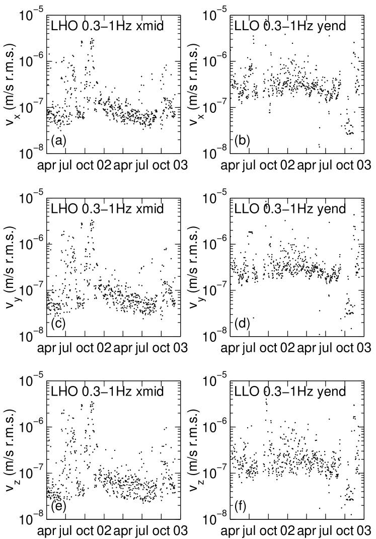
Figure 7: Time series of the three cartesian components of ground velocity at the X midstation at Hanford (left column) and the Y endstation at Livingston (right column) in the 0.3–1 Hz frequency band. Each point is the r.m.s. over 1 day. The labeling of the dependent variable axis on the plots are the same as described in the caption of figure 4.

Figure 8: A cumulative histogram of the fraction of 1 minute duration measurements of r.m.s. velocity in the 0.3–1 Hz band yielding a result greater than the abscissa. The results are for the same seismometers and directions as described in the caption for figure 5 The number of points in the histograms is 705302 (710434) for the Livingston horizontal (vertical) histograms and 678407 (678531) for the Hanford horizontal (vertical) histograms.

Figure 7 shows the three components of r.m.s. slab velocity in this band measured by the Hanford X midstation and the Livingston Y endstation seismometers. Figure 8 gives cumulative histograms of the $x$ and $z$ components of slab velocity in the Livingston and Hanford corner stations, which were representative of the results from the other buildings. Table 2 shows summary data for all seismometers and axes, using the same percentile values as measured for the 0.1–0.3 Hz band described above.

There is some evidence for a component of the slab motion having an annual modulation, which is expected given that this frequency band encompasses the upper part of the frequency band for secondary microseisms. The percentile velocities from the table are a factor of 2–3 larger at Livingston than at Hanford. The ratio of vertical to horizontal noise amplitude is about 1.5 for both sites. The two components of horizontal motion at each seismometer have about the same amplitude for each seismometer.

The time series plots from Hanford show some large positive excursions, a factor of 10–30 in r.m.s. parallel to all axes between May and October 2001. We speculate that these excursions may have been caused by off site earth moving equipment near the Hanford interferometer, although we are unable to provide further evidence in support of this possibility. The Livingston time series data shows a period of lower amplitude in September 2002. These are bad data due to some intrusive repairs and upgrades in the data acquisition system.

Table 2: Table of 50th, 90th, and 95th percentile measured r.m.s. ground velocities in three locations at each LIGO site, after applying a 0.3–1 Hz bandpass filter. In the percentage of one minute measurements given at the head of each column, the measured ground velocity in this band was less than the tabulated value.

• 0.3–1 Hz band
  site	building	axis	velocity percentile ($\mu\rm m\,s^{-1}$)
  			50%	90%	95%
  Livingston	Corner	$x$	0.23	0.45	0.63
  		$y$	0.22	0.45	0.63
  		$z$	0.14	0.38	0.56
  	X end	$x$	0.22	0.45	0.65
  		$y$	0.21	0.44	0.63
  		$z$	0.13	0.36	0.57
  	Y end	$x$	0.25	0.59	0.83
  		$y$	0.25	0.70	1.4
  		$z$	0.15	0.41	0.61
  Hanford	Corner	$x$	0.051	0.10	0.13
  		$y$	0.041	0.093	0.12
  		$z$	0.031	0.066	0.088
  	X mid.	$x$	0.060	0.12	0.17
  		$y$	0.046	0.11	0.14
  		$z$	0.035	0.071	0.098
  	Y mid.	$x$	0.057	0.19	0.29
  		$y$	0.044	0.15	0.22
  		$z$	0.032	0.065	0.081

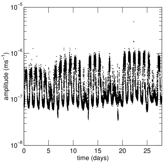
Figure 9: Time series of r.m.s. noise in the 1–3 Hz band taken from a horizontal ($x$) axis of the Livingston X endstation seismometer. The duration of the plot is 28 days. The spikes correspond to daytime, the smaller spikes every 7 days are Sundays. The start time of the plot is November 6th 2001, UTC 07:39:56. The large spikes are in groups of 6 for the weekdays plus Saturday, with the exception of the 3rd group for which the 4th spike is unusually small. This is Thanksgiving day.

Figure 10: Time series of the three cartesian components of ground velocity at the X midstation at Hanford (left column) and the Y endstation at Livingston (right column) in the 1–3 Hz frequency band. Each point is the r.m.s. over 1 day. The labeling of the dependent variable axes of the plots is the same as described in the caption of figure 4.

Figure 11: Cumulative histograms of the fraction of 1 minute duration measurements of r.m.s. velocity in the 1–3 Hz band yielding a result greater than the abscissa. The four plots compare the slab velocity components at parallel to the interferometer arms at the Livingston and Hanford corner stations, and the same components at the Livingston end stations and the Hanford mid stations. The plot legends give the number of events populating the histograms.

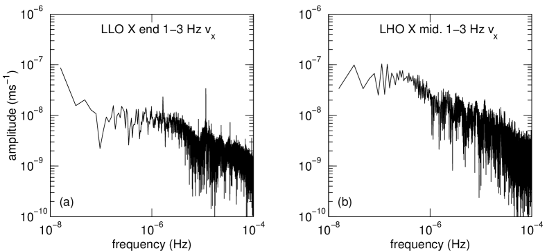
Figure 12: Amplitude spectra of the time series output of the 1–3 Hz filtered r.m.s. measurements from a horizontal ($x$) component of the Livingston X endstation seismometer and a horizontal ($x$) component of the Hanford X midstation seismometers.

Table 3: Table of 50th, 90th, and 95th percentile measured r.m.s. ground velocities in three locations at each LIGO site, after applying a 1–3 Hz bandpass filter. In the percentage of one minute measurements given at the head of each column, the measured ground velocity in this band was less than the tabulated value.

• 1–3 Hz band
  site	building	axis	velocity percentile ($\mu\rm m\,s^{-1}$)
  			50%	90%	95%
  Livingston	Corner	$x$	0.087	0.32	0.40
  		$y$	0.093	0.30	0.38
  		$z$	0.12	0.56	0.75
  	X end	$x$	0.12	0.34	0.47
  		$y$	0.21	0.40	0.53
  		$z$	0.13	0.39	0.55
  	Y end	$x$	0.16	0.65	1.1
  		$y$	0.16	0.75	1.7
  		$z$	0.20	0.72	1.1
  Hanford	Corner	$x$	0.042	0.079	0.12
  		$y$	0.042	0.083	0.12
  		$z$	0.020	0.059	0.097
  	X mid.	$x$	0.035	0.077	0.13
  		$y$	0.033	0.077	0.12
  		$z$	0.019	0.045	0.077
  	Y mid.	$x$	0.037	0.15	0.31
  		$y$	0.032	0.10	0.36
  		$z$	0.033	0.10	0.36

4.3 The 1–3 Hz Frequency Band

Slab motion in the 1–3 Hz band contains no appreciable contribution from secondary microseisms. The dominant contribution to slab motion in this band derives from human activies involving vehicles and machinery in the vicinity of the sites. Figure 9 shows one minute measurements of the $x$ component of slab velocity in the Livingston Y endstation over 28 days commencing at 07:39:56 UTC on November 6th 2001. The measured velocity is dominated by a strong day night modulation whose amplitude decreases for one day per week. The higher noise level in the daytime is due to human activity. The lower amplitude of the daytime peak is on Sundays. The 16th day of this data set was Thanksgiving, which has a lower level of daytime slab noise than on the other weekdays.

This frequency band is particularly important to the interferometers, since two of the resonances of the vibration isolation stack under each LIGO optic are at 1.2 Hz and 2.1 Hz. Excess ground motion in this frequency range can ring up these resonances, adding to the force noise on the mirrors, which increases the fraction of the dynamic reserve of the control systems utilized in surpressing mirror motions. By this mechanism, 1–3 Hz ground motion often causes lock loss, particularly at Livingston. Also, even when lock is not lost, the resultant increased r.m.s. deviation from the dark fringe adds shot noise and increases the sensitivity to other technical noises.

Figure 10 shows time series of the cartesian components of slab velocity for one seismometer at each site. There is no evidence for annual modulation. Because each data point on these plots represents an r.m.s. reading over a whole day, the modulation during the day due to human activity is invisible. On the noisiest days at Livingston, the slab velocity averages $\mathrm{3~{}\mu m/s}$. There are also obvious periods of increased human activity lasting on the order of a month. It is now known that the Livingston excess noise is caused primarily by logging activities in the vicinity of the site. There is also a contribution from the town of Livingston. There is no evidence here for a trend towards increasing r.m.s. slab velocity over the 613 days of this measurement.

Figure 11 shows cumulative histograms of 1–3 Hz seismic noise. The four plots give results from the two seismometer axes parallel to each interferometer arm at each site. Table 3 gives percentile velocities in all seismometers and axes. The noisiest station is the Y endstation at Livingston. Measuring parallel to the beam pipe, the 90th percentile slab velocity is 0.75, a factor of 5 greater than the noisiest data from Hanford, which is the $x$ axis of the Y midstation velocity. The ratio of the 90th percentile velocities of the noisiest horizontal Livingston seismometer axis to the quietest horizontal Hanford seismometer axis is about 10.

Figure 12 shows amplitude spectra from the $x$ axes of the Livingston X endstation and the Hanford X midstation. The strong peaks at frequencies of $\mathrm{12\mu Hz}$ and $\mathrm{1.6\mu Hz}$ correspond to periods of 1 day and 1 week respectively. One day and one week periodicities are not evident in the data fron the Hanford X midstation. This is the seismometer that is furthest from the roads out of the three used in this study. Some day-night variation can be seen in time series from the Y midstation, but it is much weaker than that seen at Livingston.

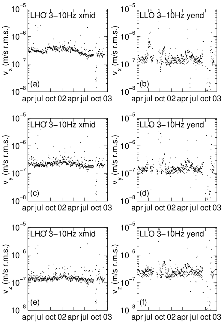
Figure 13: Time series of the three cartesian components of ground velocity at the X midstation at Hanford (left column) and the Y endstation at Livingston (right column) in the 3–10 Hz frequency band. Each point is the r.m.s. over 1 day. The labeling of the dependent variable of the plots is the same as described in the caption of figure 4.

Figure 14: A cumulative histogram of the fraction of 1 minute duration measurements of r.m.s. velocity in the 3–10 Hz band yielding a result greater than the abscissa. The plot on the left gives results for a horizontal ($x$) and the vertical ($z$) component measured in the Livingston corner station. The plot on the right gives results for a horizontal ($x$) and the vertical ($z$) component at the Hanford corner station. The number of points in the histograms is 726730 (727500) for the Livingston horizontal (vertical) axis histograms and 699145 (703879) for the Hanford horizontal (vertical) axis histograms.

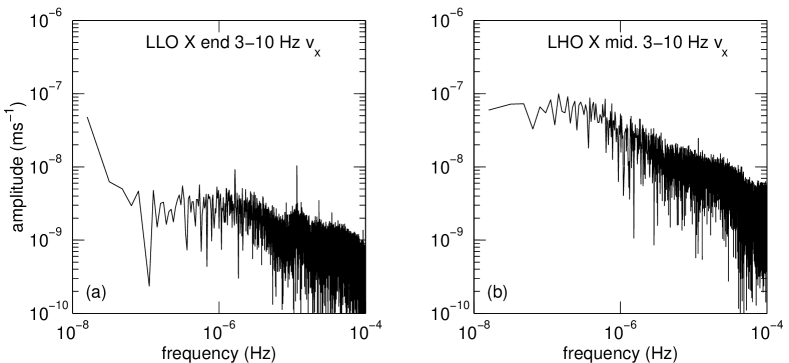
Figure 15: Amplitude spectra of the time series output of the 3–10 Hz filtered r.m.s. measurements for a horizontal ($x$) axis of the Livingston X endstation and the Hanford X midstation seismometers.

4.4 The 3–10 Hz Frequency Band

Like the 1–3 Hz band, the 3–10 Hz encompasses a resonance, at 6.3 Hz, of the vibration isolation stack. This frequency band shows the day night modulation associated with human activity, but at a lower level than was seen in the 1–3 Hz band. Figure 13 shows r.m.s. measured over one day of 3–10 Hz slab velocity in the Hanford X midstation and the Livingston Y endstation. Table 4 shows the 50th, 90th, and 95th percentile slab velocities in all seismometers and axes. Figure 14 shows the cumulative histograms of slab velocities at the Livingston and Hanford corner station $x$ and $z$ axes.

In the 3–10 Hz band, slab velocities at Hanford are 5–50 % higher than at Livingston. There is much larger variation between the slab velocities measured in different buildings at the same site than for the other bands. We also see greater difference between measured velocity percentiles along different axes of the same seismometer, suggesting that specific close sources of vibration might be the cause of ground motion at these frequencies. At Livingston, in contrast to the other frequency bands, the vertical component of slab velocity is at least as large as the horizontal components. The most extreme case, the Livingston corner station, is illustrated in figure 14, where the $z$ component of slab motion is three times higher than the $x$ and $y$ components. An anomolously large vertical slab motion in the corner station is also seen at Hanford. This pattern suggests that some local source of vibration is exciting the slab in the corner stations at both sites. The corner buildings contain more mechanical equipment than the arm buildings. We do not think it likely that this effect is due to movement and activity of the LIGO scientists in the corner stations. In our experience, human activities would also lead to an excess in the 1–3 Hz band, which is not seen.

Table 4: Table of 50th, 90th, and 95th percentile measured r.m.s. ground velocities in three locations at each LIGO site, after applying a 3–10 Hz bandpass filter. In the percentage of one minute measurements given at the head of each column, the measured ground velocity in this band was less than the tabulated value.

• 3–10 Hz band
  site	building	axis	velocity percentile ($\mu\rm m\,s^{-1}$)
  			50%	90%	95%
  Livingston	Corner	$x$	0.060	0.11	0.16
  		$y$	0.081	0.13	0.20
  		$z$	0.25	0.38	0.61
  	X end	$x$	0.15	0.24	0.33
  		$y$	0.22	0.30	0.39
  		$z$	0.25	0.38	0.46
  	Y end	$x$	0.094	0.34	0.52
  		$y$	0.099	0.28	0.45
  		$z$	0.15	0.39	0.56
  Hanford	Corner	$x$	0.10	0.15	0.21
  		$y$	0.11	0.17	0.23
  		$z$	0.20	0.28	0.40
  	X mid.	$x$	0.29	0.41	0.44
  		$y$	0.20	0.28	0.32
  		$z$	0.12	0.17	0.21
  	Y mid.	$x$	0.15	0.26	0.57
  		$y$	0.19	0.28	0.66
  		$z$	0.14	0.19	0.21

5 Conclusions and Future Work

We have presented a detailed study of the ground noise properties of the slabs supporting the LIGO vacuum system and optical components. For the lower frequency bands investigated, between 0.1 and 1 Hz, the noise is dominated by microseismic waves. Between 1 and 10 Hz, the dominant noise sources are due to human activity in the vicinity of the instruments.

The most critical band for operation of the interferometer is the 1–3 Hz band, in which the r.m.s. slab velocity parallel to the interferometer arms is typically four times as high at Livingston as at Hanford. The noise level increases in the daytime, and is due to human activity, particularly logging machinery close to the Livingston site. We see no long term trend of increasing slab velocity over the 613 day duration of these measurements at Livingston. Slab velocity in the Livingston Y endstation is a factor of 2 to 2.5 larger than in the X endstation or the corner station. Seismic filtering retrofits [19] should take into account the particularly noisy environment in this building.

In the 3–10 Hz band the effects of human activity are still seen, but are typically at a lower level than in the 1–3 Hz band. Slab noise parallel to the ground appears less isotropic than in the 1–3 Hz band, and slab velocities are typically larger in the arm buildings than the corner stations at both sites.

In both the 1–3 Hz and 3–10 Hz bands at Livingston, the vertical component of slab velocity is equal to or larger than the horizontal components. For these same bands at Hanford, the vertical component is larger in the corner stations but smaller in the arm buildings than the horizontal components.

The two frequency bands below 1 Hz are dominated by the secondary microseism. We see evidence for annual modulation of the slab velocity in this band. A longer data set is needed to determine the amplitude and stationarity of this annual modulation. The ratio of vertical to horizontal slab motion at Livingston is 0.5 to 0.7 in the 0.1–0.3 Hz band, whereas at Hanford this ratio is 1–1.3. In the 0.3–1 Hz band, the 90th percentile vertical component of slab velocity is typically smaller than the horizontal components at both sites.

Future enhancements of this analysis are planned. A detailed study of the ratio of peak slab velocities to the r.m.s. levels determined in this study would be useful in designing upgrades to improve isolation of the LIGO optics from the ground. A specialized study focusing on ground motion in the 1–3 Hz frequency band at Livingston during train passages is planned, and would provide useful data for instrument upgrades designed to improve interferometer isolation from ground disturbances.

References

References

- [1] Abramovici A, Althouse W, Drever R W P ,Gursel Y, Kawamura S, Raab F J, Shoemaker D, Sievers L, Spero R, Thorne K S, Vogt R E, Weiss R, Whitcomb S E and Zucker M E 1992 Science 256 325
- [2] Abbott B et al15th August 2003 gr-qc/0308043.
- [3] Fritschel P, Bork R, Gonzalez G, Mavalvala N, Ouimette D, Rong H, Sigg D and Zucker M 2001 Applied Optics 40 4988
- [4] Giaime J A, Daw E J, Weitz M, Adhikari R, Fritschel P, Abbott R, Bork R and Heefner J 2003 Rev. Sci. Instrum.44 218
- [5] Adhikari R, Gonzalez G, Landry M and O’Reilly B 2003 Class. Quantum Grav.20 S903-S914
- [6] Evans M, Mavalvala N, Fritschel P, Bork R, Bhawal B, Gustafson R, Kells W, Landry M, Sigg D Weiss R, Whitcomb S, Yamomoto H 2002 Optics Letters 27 no. 8 598-600
- [7] Giaime J, Saha P, Shoemaker D and Sievers L 1996 Rev. Sci. Instrum.67 no. 1 208-214
- [8] Hoitink D J, Burk K W, Ramsdell J V and Shaw W J 2003 Hanford Site Climatological Summary 2002 with Historical Data PNL-14242, Pacific Northwest Laboratory, Richland, Washington.
-
[9]
Data from the Hanford Groundwater Monitoring Project, Battelle’s Pacific
Northwest Division, P.O. Box 999, MSIN K6-96, Richland, WA 99352.
http://hanford-site.pnl.gov/groundwater/reports/gwrep98/images/f33-1f.gif -
[10]
Population data taken from the 2000 U.S. census.
Livingston data at http://www.epodunk.com/cgi-bin/popInfo.php?locIndex=3451,
Tri Cities data at
http://kennewick.areaconnect.com/statistics.htm,
http://richland.areaconnect.com/statistics.htm,
http://pasco.areaconnect.com/statistics.htm. - [11] Data supplied by the Louisiana Geological Survey, Louisiana State University, Baton Rouge, LA, 70803, http://www.lgs.lsu.edu/gengeo.htm
- [12] Data supplied by the Louisiana Office of State Climatology, Louisiana State University, Baton Rouge, LA, 70803, http://www.losc.lsu.edu
- [13] Bork R, Shoemaker D, Sigg D and Zweizig J 1999, LIGO internal technical report LIGO-T990018-A-D.
- [14] Guralp Systems, Unit 2-3 Midas House, Calleva Park, Aldermaston, Reading, Berkshire, U.K.
- [15] Brandywine Communications, 2230 South Fairview Street, Santa Ana, CA, U.S.A.
- [16] ICS Ltd., 5430 Canotek Road, Gloucester, Ontario, Canada.
- [17] Wind River, 500 Wind River Way, Alameda, California, U.S.A.
- [18] Cessaro R, 1994, B.S.S.A. 84 no. 1 142-148
- [19] Abbot R et al2003 ‘Seismic Isolation Enhancements for Initial and Advanced LIGO’ Class. Quantum Grav.20, ISSN 0264-9381. In Press.