BAROTROPIC FRW COSMOLOGIES WITH A DIRAC-LIKE PARAMETER

H.C. ROSU   and R. LÓPEZ-SANDOVAL

Potosinian Institute of Science and Technology,

IPICyT, Apdo Postal 3-74 Tangamanga, 78231 San Luis Potosí, Mexico

Using the known connection between Schroedinger-like equations and Dirac-like equations in the supersymmetric context, we discuss an extension of FRW barotropic cosmologies in which a Dirac mass-like parameter is introduced. New Hubble cosmological parameters $\rm H_{K}(\eta)$ depending on the Dirac-like parameter are plotted and compared with the standard Hubble case $\rm H_{0}(\eta)$. The new $\rm H_{K}(\eta)$ are complex quantities. The imaginary part is a supersymmetric way of introducing dissipation and instabilities in the barotropic FRW hydrodynamics.

1 - Introduction

The scale factor ${\rm a(t)}$ of a FRW metric is a function of the comoving time ${\rm t}$ obeying the Einstein-Friedmann dynamical equations supplemented by the (barotropic) equation of state of the cosmological fluid

$${\rm\frac{\ddot{a}}{a}=-\frac{4\pi G}{3}(\rho+3p)}~{},$$ (1)

$${\rm\left(\frac{\dot{a}}{a}\right)^{2}=\frac{8\pi G\rho}{3}-\frac{\kappa}{a^{2}}~{},}$$ (2)

$${\rm p=(\gamma-1)\rho,}$$ (3)

where $\rho$ and ${\rm p}$ are the energy density and the pressure, respectively, of the perfect fluid of which a classical universe is usually assumed to be made of, $\kappa=0,\pm 1$ is the curvature index of the flat, closed, open universe, respectively, and $\gamma$ is the constant adiabatic index of the cosmological fluid. A simple Riccati route of solving the system of eqs. (1)-(3) proposed by Faraoni,^? has been used by Rosu to develop a factorization (nonrelativistic supersymmetry) approach of the barotropic FRW cosmologies,^? in which a simple explanation for a currently accelerating universe,^? in terms of ‘Darboux fluids’ with effective adiabatic indices is possible.

In this work, we first briefly review the supersymmetric factorization methods for barotropic FRW cosmologies in section 2. Next, in section 3, we present Dirac-like (first-order) coupled differential equations and their associated second-order differential equations. This allows a simple extension of barotropic FRW cosmologies that include a Dirac mass-like constant parameter ${\rm K}$.

2 - Supersymmetric methods

Combining the equations (1)-(3) and using the conformal time variable $\eta$ defined by ${\rm dt=a(\eta)d\eta}$ one gets the equation

$${\rm\frac{a^{{}^{\prime\prime}}}{a}+(c-1)\left(\frac{a^{{}^{\prime}}}{a}\right)^{2}+c\kappa=0~{}.}$$ (4)

where ${\rm c=\frac{3}{2}\gamma-1}$. The case $\kappa=0$ is directly integrable,^? and will be skipped henceforth. The logarithmic derivative ${\rm H_{0}=\frac{a^{{}^{\prime}}}{a}}$ is the Hubble parameter of the universe which is a fundamental cosmological quantity ever since Hubble’s discovery of the expansion of the universe in1929. Interestingly, passing to the function ${\rm H_{0}}$ in Eq. (4) the following Riccati equation is obtained

$${\rm H^{{}^{\prime}}_{0}+cH^{2}_{0}+\kappa c=0~{}.}$$ (5)

Employing now ${\rm H_{0}=\frac{1}{c}\frac{w^{{}^{\prime}}_{\kappa}}{w_{\kappa}}}$ one gets the very simple second order differential equation

$${\rm w^{{}^{\prime\prime}}_{\kappa}+\kappa c^{2}w_{\kappa}=0~{}.}$$ (6)

For $\kappa=1$ the solution of the latter is ${\rm w_{1}=W_{1}\cos(c\eta+d)}$ , where ${\rm d}$ is an arbitrary phase, implying ${\rm a_{1}(\eta)=A_{1}[\cos(c\eta+d)]^{1/c}~{},}$ whereas for $\kappa=-1$ one gets ${\rm w_{-1}=W_{-1}{\rm sinh}(c\eta)}$ and therefore ${\rm a_{-1}(\eta)=A_{-1}[{\rm sinh}(c\eta)]^{1/c}}~{},$ where ${\rm W_{\pm 1}}$ and ${\rm A_{\pm 1}}$ are amplitude parameters.

The point now is that the particular Riccati solutions ${\rm H_{0}^{+}=-\tan c\eta}$ and ${\rm H_{0}^{-}={\rm coth}c\eta}$ for $\kappa=\pm 1$, respectively, are closely related to the common factorizations of the Schrödinger equation. Indeed, Eq. (6) can be written

$${\rm w^{{}^{\prime\prime}}-c(-\kappa c)w=0}$$ (7)

and also in factorized form using Eq. (6) one gets

$${\rm\left(\frac{d}{d\eta}+cH_{0}\right)\left(\frac{d}{d\eta}-cH_{0}\right)w=w^{{}^{\prime\prime}}-c(H_{0}^{{}^{\prime}}+cH_{0}^{2})w=0}~{}.$$ (8)

To fix the ideas, we shall call Eq. (8) the bosonic equation. On the other hand, the supersymmetric partner (or fermionic) equation of Eq. (8) will be

$${\rm\left(\frac{d}{d\eta}-cH_{0}\right)\left(\frac{d}{d\eta}+cH_{0}\right)w_{f}=w^{{}^{\prime\prime}}_{f}-c(-H_{0}^{{}^{\prime}}+cH_{0}^{2})w_{f}={\rm w^{{}^{\prime\prime}}_{f}-c\cdot c_{\kappa,susy}w_{f}=0}}~{}.$$ (9)

Thus, one can write

$${\rm c_{\kappa,susy}(\eta)=-H_{0}^{{}^{\prime}}+cH_{0}^{2}=\left\{\begin{array}[]{ll}c(1+2{\rm tan}^{2}c\eta)&\mbox{if $\kappa=1$}\\ c(-1+2{\rm coth}^{2}c\eta)&\mbox{if $\kappa=-1$}\end{array}\right.}$$

for the supersymmetric partner adiabatic index. The solutions are $\rm w_{f}=\frac{c}{\cos(c\eta+d)}$ and $\rm w_{f}=\frac{c}{sinh(c\eta)}$ for $\kappa=1$ and $\kappa=-1$, respectively.

3 - Dirac-like formalism

The Dirac equation in the susy nonrelativistic formalism has been discussed by Cooper et al,^? already in 1988. They showed that the Dirac equation with a Lorentz scalar potential is associated with a susy pair of Schroedinger Hamiltonians. This result has been used later by many other authors. Here we make an application to barotropic FRW cosmologies that we find not to be a trivial exercise except for the uncoupled ‘zero-mass’ case (subsection 3.1).

3.1- Let’s introduce now the following two Pauli matrices

$$\alpha=-i\sigma_{y}=-i\left(\begin{array}[]{cc}0&-i\\ i&0\end{array}\right)\qquad{\rm and}\quad\beta=\sigma_{x}=\left(\begin{array}[]{cc}0&1\\ 1&0\end{array}\right)$$

and write a cosmological Dirac equation

$${\rm{\cal H}_{0}^{{\rm FRW}}W=[\sigma_{y}D_{\eta}+\sigma_{x}(icH_{0})]W=0}~{},$$ (10)

where $W=\left({\rm\begin{array}[]{cc}w_{1}\\ w_{2}\end{array}}\right)$ is a two component ‘zero-mass’ spinor. This is equivalent to the following decoupled equations

$${\rm D}_{\eta}w_{1}+{\rm cH_{0}}w_{1}=0$$ (11)

$$-{\rm D}_{\eta}w_{2}+{\rm cH_{0}}w_{2}=0~{}.$$ (12)

Solving these equations one gets $w_{1}\propto 1/\cos({\rm c}\eta)$ and $w_{2}\propto\cos({\rm c}\eta)$ for $\kappa=1$ cosmologies and $w_{1}\propto 1/{\rm sinh}({\rm c}\eta)$ and $w_{2}\propto{\rm sinh}({\rm c}\eta)$ for $\kappa=-1$ cosmologies. Thus, we obtain

$$W=\left({\rm\begin{array}[]{cc}w_{1}\\ w_{2}\end{array}}\right)=\left({\rm\begin{array}[]{cc}{\rm w_{f}}\\ {\rm w_{b}}\end{array}}\right)~{}.$$

This shows that the matrix ‘zero-mass’ Dirac equation is equivalent to the two Schroedinger equations for the bosonic and fermionic components.

3.2- Consider now a “massive” Dirac equation

$${\rm H_{K}^{FRW}W=[\sigma_{y}D_{\eta}+\sigma_{x}(icH_{p}+K)]W=KW}~{},$$ (13)

where $\rm K$ may be considered the mass parameter of the Dirac spinor. Eq. (13) is equivalent to the following system of coupled equations

$${\rm D_{\eta}w_{1}+(i{\rm cH_{0}+K})w_{1}={\rm K}w_{2}}$$ (14)

$$-{\rm D_{\eta}w_{2}+({\rm icH_{0}+K})w_{2}={\rm K}w_{1}}~{}.$$ (15)

These two coupled first-order equations are equivalent to second order differential equations for the two spinor components:

The fermionic spinor component can be found directly as solutions of

$${\rm D^{2}_{\eta}w_{1}^{+}-\Big{[}c^{2}(1+2\tan^{2}c\eta)+2icK\tan c\eta\Big{]}w_{1}^{+}=0}\qquad{\rm for}\,\kappa=1$$ (16)

and

$${\rm D^{2}_{\eta}w_{1}^{-}-\Big{[}c^{2}(-1+2{\rm coth}^{2}c\eta)-2icK{\rm coth}\,c\eta\Big{]}w_{1}^{-}=0}\qquad{\rm for}\,\kappa=-1~{},$$ (17)

whereas the bosonic components are solutions of

$${\rm D^{2}_{\eta}w_{2}^{+}+\Big{[}c^{2}-2icK\tan c\eta\Big{]}w_{2}^{+}=0}\qquad{\rm for}\quad\kappa=1$$ (18)

and

$${\rm D^{2}_{\eta}w_{2}^{-}+\Big{[}-c^{2}+2icK{\rm coth}\,c\eta\Big{]}w_{2}^{-}=0}\qquad{\rm for}\quad\kappa=-1~{}.$$ (19)

The solutions of the bosonic equations are expressed in terms of the Gauss hypergeometric functions ${\rm{}_{2}F_{1}}$ in the variables ${\rm y=e^{ic\eta}}$ and ${\rm y=e^{c\eta}}$, respectively

$${\rm w_{2}^{+}=Ay^{-p}\,_{2}F_{1}\Big{[}-\frac{1}{2}(p+iq);-\frac{1}{2}(p-iq),1-p;-y^{2}\Big{]}}+$$

$${\rm By^{p}\,_{2}F_{1}\Big{[}\frac{1}{2}(p-iq),\frac{1}{2}(p+iq),1+p;-y^{2}\Big{]}}$$ (20)

and

$${\rm w_{2}^{-}=C(-1)^{-\frac{i}{2}r}y^{-ir}\,_{2}F_{1}\Big{[}-\frac{i}{2}(r+s),-\frac{i}{2}(r-s),1-r;y^{2}\Big{]}}+$$

$${\rm D(-1)^{\frac{i}{2}r}y^{ir}\,_{2}F_{1}\Big{[}\frac{i}{2}(r-s),\frac{i}{2}(r+s),1+r;y^{2}\Big{]}}~{},$$ (21)

respectively. The parameters are the following:

$${\rm p=(-1-\frac{2K}{c})^{\frac{1}{2}},\quad q=(1-\frac{2K}{c})^{\frac{1}{2}},\quad r=(-1-i\frac{2K}{c})^{\frac{1}{2}},\quad s=(-1+i\frac{2K}{c})^{\frac{1}{2}}},$$

whereas ${\rm A}$, ${\rm B}$, ${\rm C}$, ${\rm D}$ are superposition constants.

Based on these ${\rm K}$- modes, we can introduce bosonic Hubble parameters depending on the parameter ${\rm K}$

$${\rm H^{+}_{K}=\frac{1}{c}\left(\frac{D}{D\eta}\log w_{2}^{+}\right)}$$ (22)

and

$${\rm H^{-}_{K}=\frac{1}{c}\left(\frac{D}{D\eta}\log w_{2}^{-}\right)}~{},$$ (23)

and similarly for the fermionic components by changing ${\rm w_{2}^{\pm}}$ to ${\rm w_{1}^{\pm}}$ in eqs. (22) and (23), respectively.

In the small ${\rm K}$ limit, ${\rm K\rightarrow 0}$, the ordinary FRW barotropic cosmologies are obtained. The Hubble parameters corresponding to the $\rm K$- dependent bosonic modes are plotted in the Figures (1) -(4).

4 - Conclusions

We come now to the interpretation of the mathematical results that we displayed in the previous sections. The parameter $\rm K$ introduces an imaginary part in the cosmological Hubble parameter $\rm H$. Since the latter is the logarithmic derivative of the scale factor of the universe one comes to the conclusion that the supersymmetric techniques presented here are a way to consider dissipation and instabilities of barotropic FRW cosmologies.

References

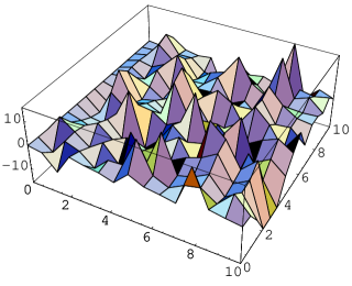
Figure 1: The real part of ${\rm H^{+}_{K}}$ obtained from the logderivative of the bosonic mode ${\rm w_{2}^{+}(y;\frac{1}{2},\frac{1}{2}})$ for ${\rm\eta}\in[0,10]$ and ${\rm K\in[0,10]}$ in the case of a radiation dominated universe (${\rm c=1}$) .

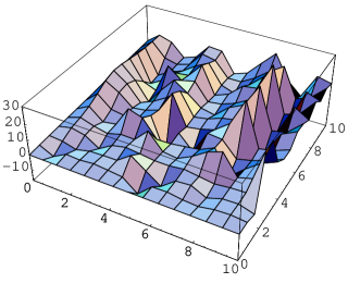
Figure 2: The imaginary part of ${\rm H^{+}_{K}}$ for the same case.

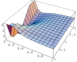
Figure 3: The real part of ${\rm H^{-}_{K}}$ calculated from the bosonic mode ${\rm w_{2}^{-}(y;\frac{1}{2},\frac{1}{2}})$ for ${\rm\eta}\in[0,1]$ and ${\rm K\in[0,2]}$ and a radiation dominated universe.

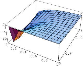
Figure 4: The imaginary part of ${\rm H^{-}_{K}}$ for the same case.

References

[1] V. Faraoni, “Solving for the dynamics of the universe”,
Am. J. Phys. 67, 732 (1999) [physics/9901006].
[2] H.C. Rosu, “Darboux class of cosmological fluids with time-dependent adiabatic indices”,
Mod. Phys. Lett. A 15, 979 (2000).
[3] S. Perlmutter et al., “Cosmology from type Ia supernovae”,
Bull. Am. Astron. Soc. 29, 1351
(1997) [astro-ph/9812473], and “Measurements of Omega and Lambda from 42
high-redshift supernovae”, astro-ph/9812133.
[4] F. Cooper, A. Khare, R. Musto, A. Wipf, “Supersymmetry and the Dirac equation”,
Ann. Phys. 187, 1 (1988). See also, R.J. Hughes, V. Alan Kostelecký, M.M. Nieto,
“Susy quantum mechanics in a first-order Dirac equation”, Phys. Rev. D 34, 1100 (1986);
Y. Nogami and F.M. Toyama, “Supersymmetry aspects of the
Dirac equation in one dimension with a Lorentz scalar potential”, Phys. Rev. A 47, 1708 (1993).