Reissner-Nordström Black Holes and Thick Domain Walls

Abstract

We solve numerically equations of motion for real self-interacting scalar fields in the background of Reissner-Nordström black hole and obtained a sequence of static axisymmetric solutions representing thick domain walls charged black hole systems. In the case of extremal Reissner-Nordström black hole solution we find that there is a parameter depending on the black hole mass and the width of the domain wall which constitutes the upper limit for the expulsion to occur.

I Introduction

Relics of cosmological phase transitions are considered to play an important role in cosmology [2]. They are signs of the high-energy phenomena which are beyond the range of contemporary accelerators. Such topological defects as cosmic strings attracted great interests due to the motivation of the uniqueness theorems for black holes and Wheeler’s conjecture black holes have no hair. Black hole cosmic string configurations were studied from different points of view [3] revealing that cosmic string could thread it or could be expelled from black hole. As far as the dilaton gravity was concerned it was also justified [4, 5] that a vortex could be treated by the remote observer as a hair on the black hole. On the other hand, for the extreme dilaton black hole one has always the expulsion of the Higgs field (the so-called Meissner effect). The problem of vortices in de Sitter (dS) background was analyzed in Ref.[6], while the behaviour of Abelian Higgs vortex solutions in Schwarzschild anti de Sitter (AdS), Kerr, Kerr-AdS and Reissner-Nordström AdS was studied in Refs.[7, 8]. The vortex solution for Abelian Higgs field Eqs. in the background of four-dimensional black string was obtained in Ref.[9].

In order to investigate the behaviour of the domain walls or cosmic strings configurations in curved spacetime a number of works use a thin wall or string approximations, i.e., infinitely thin non-gravitating membrane described by the Nambu-Goto Lagrangian. Dynamics of scattering and capture process of an infinitely thin cosmic string in the spacetime Schwarzshild black hole were elaborated in Ref.[10]. Christensen et al. [11] revealed that there existed a family of infinitely thin walls intersecting black hole event horizon. Then, the considerations were applied to the scattering of inifitely long cosmic string by a rotating black hole [12].

Nowadays, the idea that the Universe is embedded in higher-dimensional spacetime acquires much attention. The resurgence of the idea is motivated by the possibility of resolving the hierarchy problem [19], i.e., the difference in magnitudes of the Planck scale and the electroweak scales. Also the most promising candidate for a unified theory of Nature, superstring theory predicts the existence of the so-called D-branes which in turn renews the idea of brane worlds. From this theory point of view the model of brane world stems from the idea presented by Horava and Witten [20]. Namely, the strong coupling limit of $E_{8}\times E_{8}$ heterotic string theory at low energy is described by eleven-dimensional supergravity with eleventh dimension compactified on an orbifold with $Z_{2}$ symmetry. The two boundaries of spacetime are ten-dimensional planes, to which gauge theories are confined. Next in Refs.[21, 22] it was argued that six of the eleven dimensions could be consistently compactified and in the limit spacetime looked five-dimensional with four-dimensional boundary brane.
Then, it is intriguing to study the interplay between black holes and domain walls (branes). Nowadays, this challenge acquires more attention. The problem of stability of a Nambu-Goto membrane in Reissner-Nordsröm de Sitter (RN-dS) spacetime was studied in Ref.[13], while the gravitationally interacting system of a thick domain wall and Schwarschild black hole was considered in [14, 15]. Emparan et al. [16] elaborated the problem of a black hole on a topological domain wall. In [17] the dilaton black hole-domain wall system was studied analytically and it was revealed that for the extremal dilaton black hole one had to do with the expulsion of the scalar field from the black hole (the so-called Meissner effect). The numerical studies of domain wall in the spacetime of dilaton black hole was considered in Ref.[18], where the thickness of the domain wall and a potential of the scalar field $\varphi^{4}$ and sine-Gordon were taken into account.

In our paper we try to provide some continuity with the previous works [17, 18] concerning the behaviour of dilaton black hole domain wall systems, namely we shall consider the thick domain wall in the background of RN black hole.

The paper is organized as follows. Sec.II is devoted to the basic equations of the considered problem. In Sec.III we studied the RN-domain wall system both for $\varphi^{4}$ and sine-Gordon potential. We pay special attention to the extremal RN black hole case and reveal that there is an expulsion of the domain wall fields under certain conditions. In Sec.IV we concluded our investigations.

II Reissner-Nordström black hole domain wall system

In our paper we shall consider the spherically symmetric solution of Einstein-Maxwell equations described by the RN black hole metric of the form

$$ds^{2}=-\left(1-{2M\over r}+{Q^{2}\over r^{2}}\right)dt^{2}+{dr^{2}\over{\left(1-{2M\over r}+{Q^{2}\over r^{2}}\right)}}+r^{2}(d\theta^{2}+\sin^{2}\theta d\varphi^{2}).$$ (1)

The metric is asymptotically flat in the sense that the spacetime contains a data set $(\Sigma_{end},g_{ij},K_{ij})$ with gauge fields such that $\Sigma_{end}$ is diffeomorphic to ${\bf R}^{3}$ minus a ball and the following asymptotic conditions are fulfilled:

$$|g_{ij}-\delta_{ij}|+r|\partial_{a}g_{ij}|+...+r^{k}|\partial_{a_{1}...a_{k}}g_{ij}|+r|K_{ij}|+...+r^{k}|\partial_{a_{1}...a_{k}}K_{ij}|\leq{\cal O}\bigg{(}{1\over r}\bigg{)},$$ (2)

$$|F_{\alpha\beta}|+r|\partial_{a}F_{\alpha\beta}|+...+r^{k}|\partial_{a_{1}...a_{k}}F_{\alpha\beta}|\leq{\cal O}\bigg{(}{1\over r^{2}}\bigg{)}.$$ (3)

RN black hole spacetime will be the background metric on which we shall consider the domain wall equations of motion built of a self-interacting scalar field. In our investigations we use a general matter Lagrangian with real Higgs field and the symmetry breaking potential of the form as follows:

$${\cal L}_{dw}=-{1\over 2}\nabla_{\mu}\varphi\nabla^{\mu}\varphi-U(\varphi),$$ (4)

where $\varphi$ real Higgs field and the symmetry breaking potential $U(\varphi)$ has a discrete set of degenerate minima. The energy-momentum tensor for scalar field may be written as follows:

$$T_{ij}(\varphi)=-{1\over 2}g_{ij}\nabla_{m}\varphi\nabla^{m}\varphi-U(\varphi)g_{ij}+\nabla_{i}\varphi\nabla_{j}\varphi.$$ (5)

It is turned out that for the convenience we can scale out parameters via transformation $X={\varphi/\eta}$ and $\epsilon=8\pi G\eta^{2}$ [16]. The parameter $\epsilon$ is responsible for the gravitational strength and it is also connected with the gravitational interaction of the considered Higgs field. One can also define the potential $V(X)={U(\varphi)\over V_{F}}$, where $V_{F}=\lambda\eta^{4}$. All these quantities enable us to rewrite the Lagrangian for the domain wall fields in a more suitable form. Namely, it now reads

$$8\pi G{\cal L}_{dw}=-{\epsilon\over w^{2}}\bigg{[}w^{2}{\nabla_{\mu}X\nabla^{\mu}X\over 2}+V(X)\bigg{]},$$ (6)

where $w=\sqrt{{\epsilon\over 8\pi GV_{F}}}$ represents the inverse mass of the scalar after symmetry breaking. It characterizes the width of the wall defect. Just using Eq.(6) we arrive at the following expression for $X$ field:

$$\nabla_{\mu}\nabla^{\mu}X-{1\over w^{2}}{\partial V\over\partial X}=0.$$ (7)

As in Ref.[18] we shall take into account for two cases of potentials with a discrete set of degenerate minima, namely the $\varphi^{4}$ potential described by the relation

$$U_{1}(\varphi)={\lambda\over 4}(\varphi^{2}-\eta^{2})^{2},$$ (8)

and the sine-Gordon potential in the form of

$$U_{2}(\varphi)=\lambda\eta^{4}\left[1+\cos(\varphi/\eta)\right].$$ (9)

III Boundary conditions

A Boundary conditions for $\varphi^{4}$ potential

As we mentioned RN black hole spacetime is asymptotically flat, thus the asymptotic boundary solution of equation of motion for potential (8) will be the solution of equation of motion in flat spacetime. It reads as

$$\varphi_{1}(z)=\eta\tanh(\sqrt{\lambda/2}\eta z),$$ (10)

or rewritten in our units implies the following:

$$X(r,\theta)=\tanh\bigg{(}{r\cos\theta\over\sqrt{2}w}\bigg{)}$$ (11)

Thus, the equation of motion (7) for the scalar field $X$ in the considered background has the form of

$${1\over r^{2}}\partial_{r}\bigg{[}\big{(}r^{2}-2Mr+Q^{2}\big{)}\partial_{r}X\bigg{]}+{1\over r^{2}\sin\theta}\partial_{\theta}\bigg{[}\sin\theta\partial_{\theta}X\bigg{]}-{1\over w^{2}}X(X^{2}-1)=0.$$ (12)

and the energy density yields

$$E=\bigg{[}-{1\over 2}\big{(}\partial_{r}X\big{)}^{2}\bigg{(}1-{2M\over r}+{Q^{2}\over r^{2}}\bigg{)}-{1\over 2}\big{(}\partial_{\theta}X\big{)}^{2}{1\over r^{2}}\bigg{]}{w^{2}}-{1\over 4}(X^{2}-1)^{2}.$$ (13)

On the horizon of the RN black hole relation (12) gives the following boundary condition:

$${r_{+}-r_{-}\over r_{+}^{2}}\partial_{r}X\big{|}_{r=r_{+}}=-{1\over r_{+}^{2}\sin\theta}\partial_{\theta}\left[\sin\theta\partial_{\theta}X\right]+{1\over w^{2}}X(X^{2}-1),$$ (14)

where $r_{+}=M+\sqrt{M^{2}-Q^{2}}$ and $r_{-}=M-\sqrt{M^{2}-Q^{2}}$ are respectively the outer and the inner horizon of the RN black hole.
As in Ref.[18] we shall investigate only the case when the core of the wall is located in the equatorial plane $\theta=\pi/2$ of the black hole, we impose the Dirichlet boundary condition at the equatorial plane

$$X\big{|}_{\theta=\pi/2}=0,$$ (15)

as well as the regularity of the scalar field on the symmetric axis requires the Neumann boundary condition on the z-axis:

$${\partial X\over\partial\theta}\bigg{|}_{\theta=0}=0.$$ (16)

For the asymptotical flatness of the RN black hole solution we should have far from the black hole the flat spacetime solution (10). But we are limited by our computational grid which is finite, then we require the following boundary condition ought to be satisfy at the boundary of the grid

$$X\big{|}_{r=r_{max}}=\tanh\bigg{(}{r_{max}\cos\theta\over\sqrt{2}w}\bigg{)}.$$ (17)

B Boundary conditions for the sine-Gordon potential.

As far as the sine-Gordon potential (9) is concerned the flat spacetime solution is given by

$$\varphi_{2}(z)=\eta\left\{4\arctan\left[\exp(\sqrt{\lambda}\eta z)\right]-\pi\right\},$$ (18)

or in our units this is equivalent to following:

$$X(r,\theta)=4\arctan\bigg{[}\exp\bigg{(}{r\cos\theta\over w}\bigg{)}\bigg{]}-\pi.$$ (19)

In this case $V(X)=1+\cos(X)$ and $\partial V/\partial X=-\sin(X)$, and thus the equation of motion (7) takes the form

$${1\over r^{2}}\bigg{[}\partial_{r}\bigg{(}r^{2}-2Mr+Q^{2}\bigg{)}\partial_{r}X\bigg{]}+{1\over r^{2}\sin\theta}\partial_{\theta}\bigg{[}\sin\theta\partial_{\theta}X\bigg{]}+{1\over w^{2}}\sin(X)=0,$$ (20)

while the energy density is given by the relation

$$E=\bigg{[}-{1\over 2}\big{(}\partial_{r}X\big{)}^{2}\bigg{(}1-{2M\over r}+{Q^{2}\over r^{2}}\bigg{)}-{1\over 2}\big{(}\partial_{\theta}X\big{)}^{2}{1\over r^{2}}\bigg{]}{w^{2}}-1-\cos(X).$$ (21)

On the horizon from Eq.(20) one has the boundary condition as follows:

$${r_{+}-r_{-}\over r_{+}^{2}}\partial_{r}X\big{|}_{r=r_{+}}=-{1\over r_{+}^{2}\sin\theta}\partial_{\theta}\left[\sin\theta\partial_{\theta}X\right]-{1\over w^{2}}\sin(X).$$ (22)

Of course, this must be accompanied by the Dirichlet boundary conditions at the equatorial plane of the black hole (15), and the Neumann boundary condition on the symmetry axis (16), and at the outer edge of the grid

$$X\big{|}_{r=r_{max}}=4\arctan\bigg{[}\exp\bigg{(}{r_{max}\cos\theta\over w}\bigg{)}\bigg{]}-\pi.$$ (23)

Another interesting problem that should attract attention to is the case of extremal RN black hole domain wall configuration. As was revealed analitycally in Ref.[16] that for some range of parameters we should have the expulsion of the domain wall, contrary to the situation which takes places in extremal dilaton black holes [17, 18]. Simple arguments given in Ref.[16] it was revealed that for at least very small extremal black hole sitting inside the domain wall, the black hole would expel it. The mass bound for the extremal RN black hole for the expulsion was also found. For $w=1$ the black hole mass have to satisfy the condition $M^{2}<{1\over 2}$.

When $r_{+}=r_{-}$ we have to do with the extremal RN black hole and it implies the condition $Q=M$. For this case the metric has the following form:

$$ds^{2}=-\left(1-{M\over r}\right)^{2}dt^{2}+{dr^{2}\over{\left(1-{M\over r}\right)^{2}}}+r^{2}(d\theta^{2}+\sin^{2}\theta d\varphi^{2}).$$ (24)

Equation of motion for the domain wall’s scalar fields in the background of RN extremal black hole yields

$${1\over r^{2}}\partial_{r}\bigg{[}\big{(}r-M\big{)}^{2}\partial_{r}X\bigg{]}+{1\over r^{2}\sin\theta}\partial_{\theta}\bigg{[}\sin\theta\partial_{\theta}X\bigg{]}={1\over w^{2}}{\partial V\over\partial X},$$ (25)

while the relation for energy implies the following:

$$E=\bigg{[}-{1\over 2}\big{(}\partial_{r}X\big{)}^{2}\bigg{(}1-{M\over r}\bigg{)}^{2}-{1\over 2}\big{(}\partial_{\theta}X\big{)}^{2}{1\over r^{2}}\bigg{]}{w^{2}}-V(X).$$ (26)

IV Numerical calculations

A Reissner-Nordström black hole

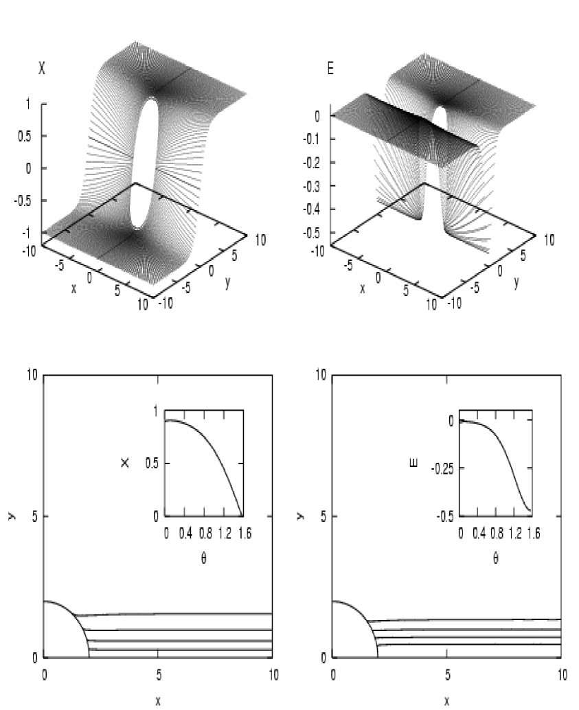
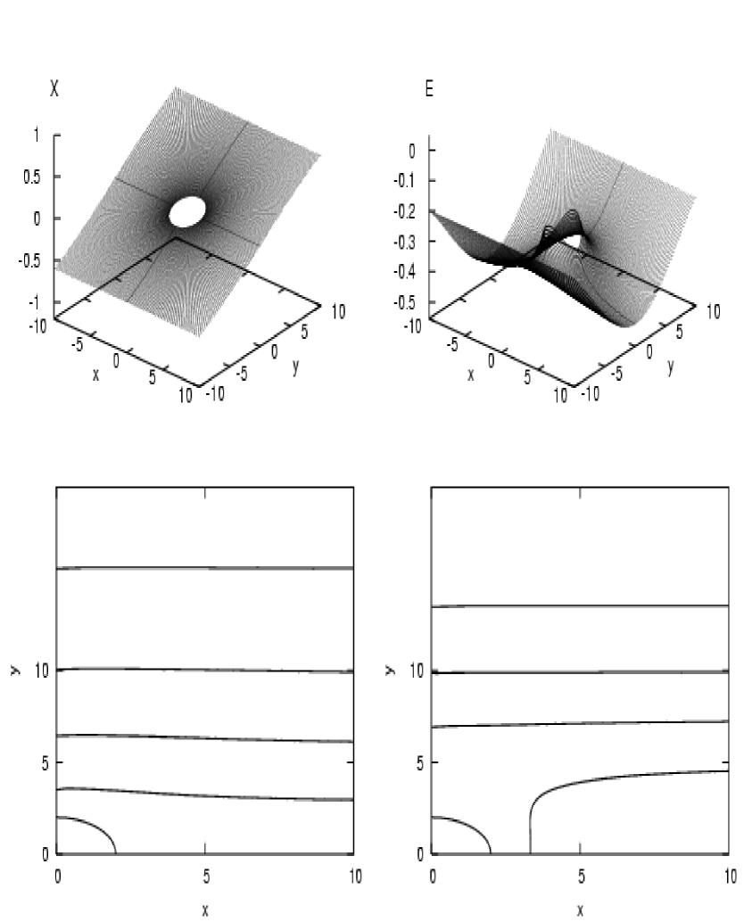
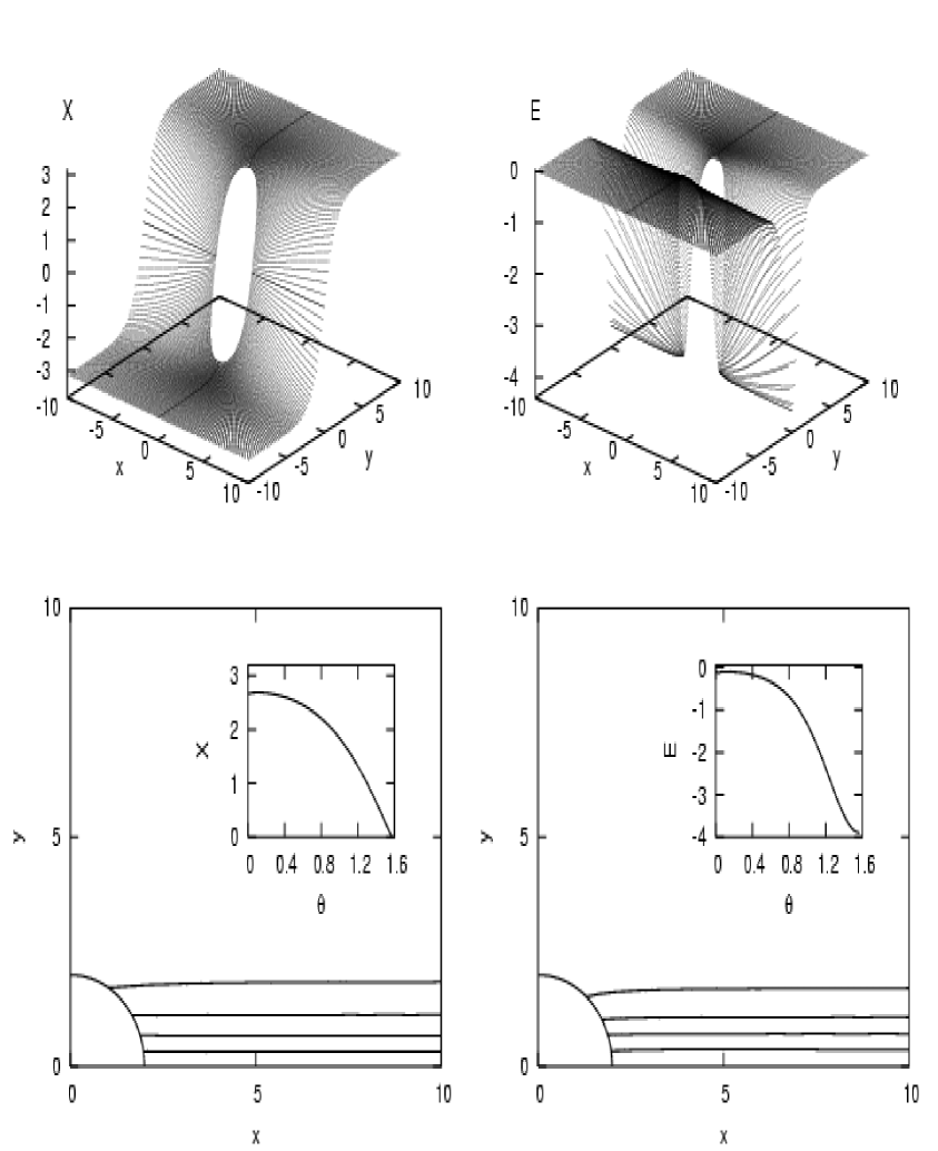
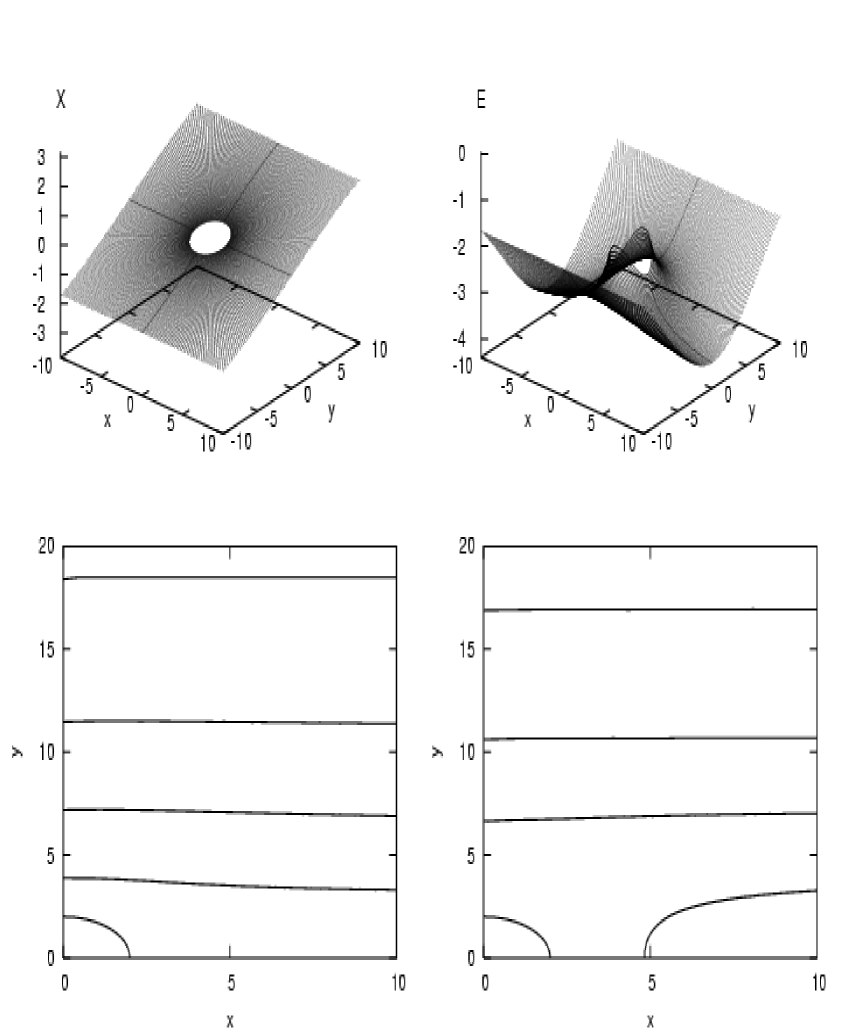
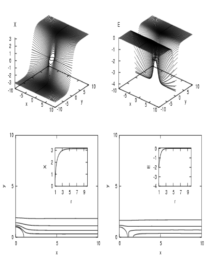
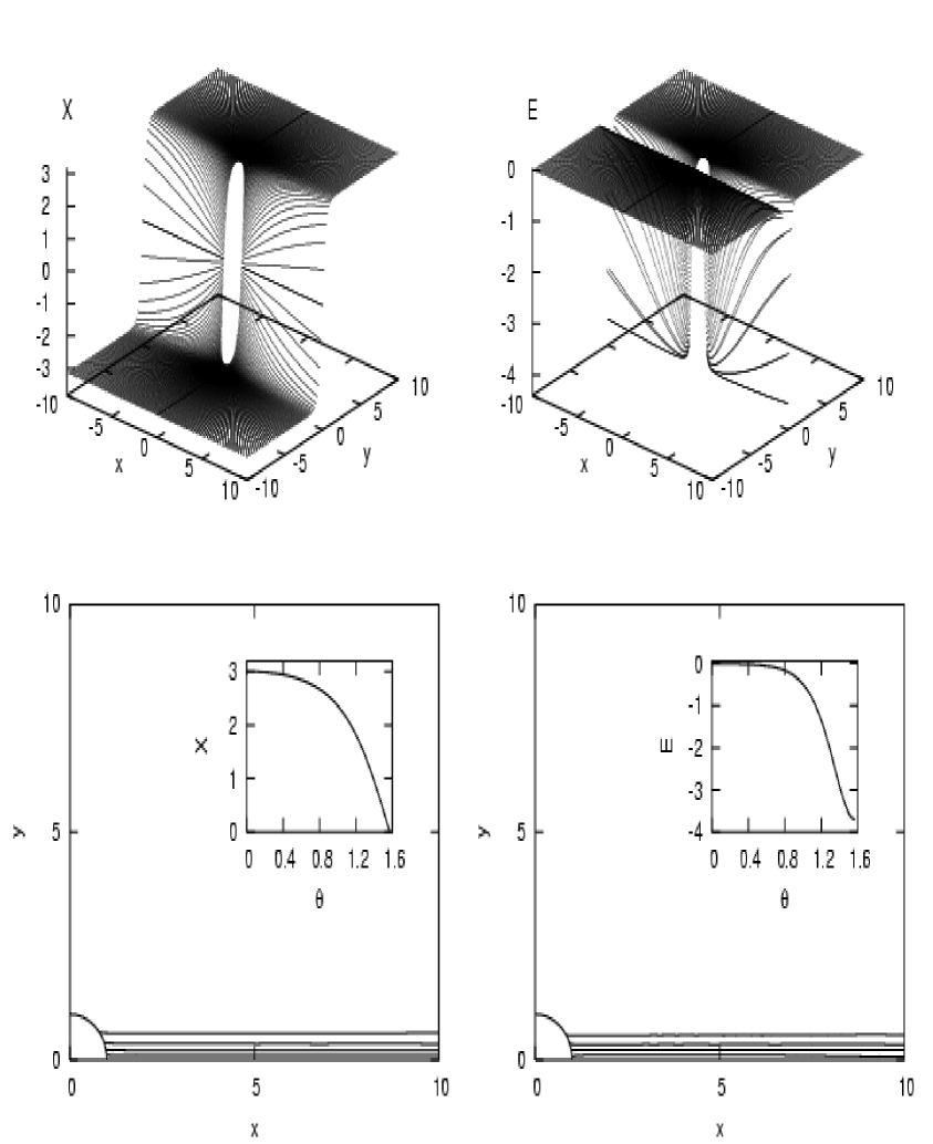
The method of solving equations of motion for the scalar fields $X$ is the same as in Ref.[18]. We applied the modified overrelaxation method in order to take into account the boundary conditions on the considered black hole horizon. Eqs. of motion will be solved on a uniformly spaced polar grid $(r_{i},\theta_{i})$ with the boundaries at $r_{min}=r_{+}$, the outer radius will be $r_{max}\gg r_{+}$ (we take usually $r_{max}=20r_{+}$ ). The angle $\theta$ changes from $0$ to $\pi/2$. Then, one approximates the derivatives with finite-difference expressions on the grid. The rest of the solution for scalar field $X$ will be obtained from the symmetry condition. The example solutions of the equation of motion for different parameters and field configurations are shown on Figs 1, 2, 3, and 4.

B An extreme Reissner-Nordström black hole

For the extremal RN black hole scalar fields on the horizon decouple from the rest of the grid and equation of motion (25) becomes an ordinary differential equation:

$$\partial_{\theta\theta}X+{1\over\tan\theta}\partial_{\theta}X-{r_{+}^{2}\over w^{2}}{\partial V\over\partial X}=0.$$ (27)

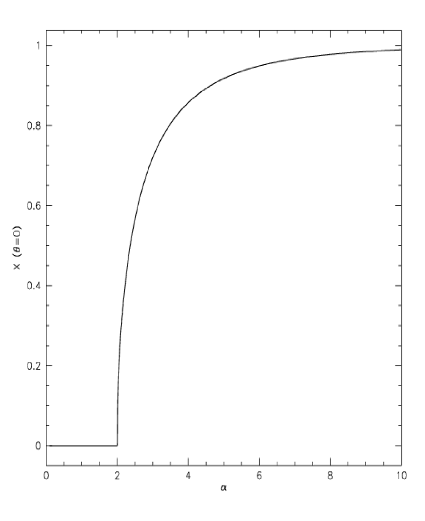
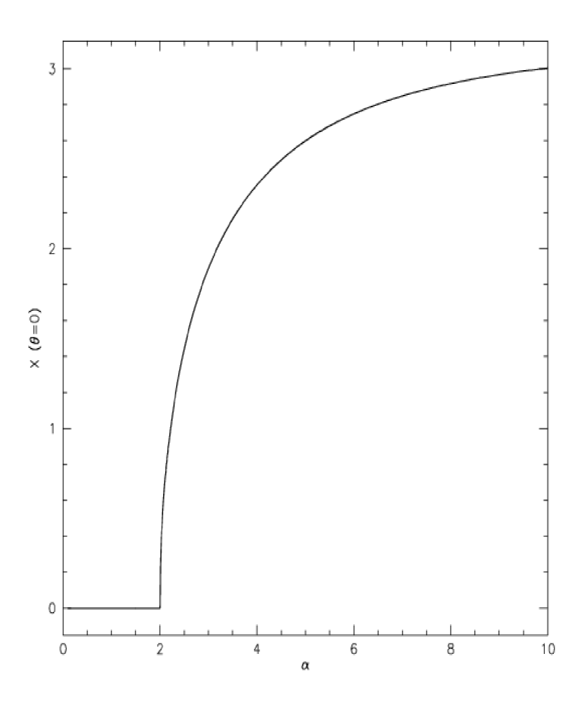
For the reasons given in [3, 18] one must carefully examine the solution on the horizon. The solution $X=0$, which corresponds to the expulsion of the field from the black hole (the Meissner effect) always solves relation (27). But sometimes other solution is possible and energetically more favourable. The previous studies envisage ([3, 18]) that the relative size of the domain wall compared to the size of the black hole becomes a factor which determines the overall behaviour of the field on the horizon. For this reason we parameterize equation (27) with parameter $\alpha\equiv{r_{+}^{2}\over w^{2}}$ and solve (27) numerically using two point boundary relaxation method ([23]). Fig. 5 shows the dependence of the scalar field $X$ on the black hole z-axis as a function of the parameter $\alpha$ for the $\varphi^{4}$ potential. Fig. 6 depicts the same dependence for the sine-Gordon potential. The difference of the scalar field behaviours is clearly visible. For the value $\alpha<2.0$ we have the field expulsion, while for $\alpha>2.0$ the field pierces the horizon of the extremal RN black hole. The value of the critical parameter is the same in both cases, which is easily understood when one considers the series expansion of the $\partial V/\partial X$ around zero and neglects higher terms.

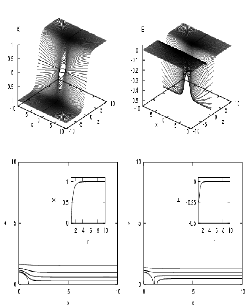
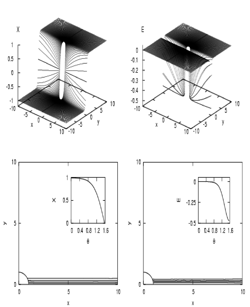
Figs 7, 8, 9, 10 show examples of the field configuration for various combinations of the $\alpha$ parameter and the adequate potentials.

Summing it all up we conclude that the numerical studies of the scalar domain wall field in the vicinity of RN black hole reveal that for the extremal case one has not always expulsion of the fields from the black hole. This phenomenon depends on the value of the black hole radius $r_{+}$ and the width of the domain wall. If the parameter $\alpha<2.0$ we have expulsion of the scalar field $X$ while for $\alpha>2.0$ the scalar fields penetrate the extremal RN black hole horizon. The domain wall extremal RN black hole system was studied analytically in Ref.[16]. By simple argument it was revealed that at least small extremal RN black holes sitting inside the domain wall would expel it. Then a more precise bound on the mass of the considered black hole was established. For $M^{2}<1/2$ the defect’s field cease to penetrate the black hole horizon, but for $M^{2}>1/2$ one has no such expelling. In Ref.[16] the considerations were conducted for the case of the domain wall’s width equaled to $1$.

On the contrary, in the case of extremal dilaton black hole domain wall system it was shown that one had always expulsion of the scalar field [17, 18]. It turned out that the simplest generalization of Einstein-Maxwell theory by adding massless dilaton field dramatically changed the structure of the extremal black hole. The similar situation takes place when one consideres anothe topological defect, i.e., cosmic string. For extremal dilaton black holes we observe always expulsion of the fields [4].

V Conclusions

In our paper we elaborated the problem of thick domain walls in the background of a spherically symmetric solution of Einstein-Maxwell field equations. The domain wall equations of motion were built of a self-interacting real scalar fields with the symmetry breaking potential having a discrete set of degenerate minima. Using the modified overrelaxation method modified in order to comprise the boundary conditions of the scalar field $X$ on the black hole horizon we solved numerically Eqs. of motion for $\varphi^{4}$ and sine-Gordon potentials. All our solutions depended on the parameter $w=1/\sqrt{\lambda}\eta$ which was responsible for the domain wall thickness. We revealed the systems of axisymmetric scalar field configurations representing thick domain wall in the nearby of RN black hole for both kinds of potentials. We paid special attention to the extremal RN black hole solution. We parametrized the equations of motion with the parameter $\alpha={r_{+}^{2}\over w^{2}}$ and solved it by means of the two-point boundary relaxation method. For $\alpha<2$ one observed the complete expulsion of the scalar field $X$ from the extremal RN black hole (the so-called Meissner effect), while for $\alpha>2$ the domain wall’s field penetrated the extremal RN black hole horizon. This behaviour is in contrast to the behaviour of scalar field in the background of the extremal dilaton black hole, where we have a complete expulsion of the scalar fields.

Acknowledgements:
M.R. was supported in part by KBN grant No. 2 P03B 124 24.

FIG. 1.: The field X (left panels) and the energy E (right panels) for the $\phi^{4}$ potential and the Reissner-Nordström black hole. Isolines on bottom panels are drawn for $0.2$, $0.4$, $0.6$ and $0.8$ for the field X and for $-0.1$, $-0.2$, $-0.3$ and $-0.4$ for the energy. Inlets in bottom plots show the value of the fields on the black hole horizon. Black hole has $M=1.0$, $Q=0.1$ and the domain width is $w=1.0$.

FIG. 2.: The field X (left panels) and the energy E (right panels) for the $\phi^{4}$ potential and the Reissner-Nordström black hole. Isolines on bottom panels are drawn for $0.2$, $0.4$, $0.6$ and $0.8$ for the field X and for $-0.1$, $-0.2$, $-0.3$ and $-0.4$ for the energy. Black hole has $M=1.0$, $Q=0.1$ and the domain width is $w=10$.

FIG. 3.: The field X (left panels) and the energy E (right panels) for the sine-Gordon potential and the Reissner-Nordström black hole. Isolines on bottom panels are drawn for $0.2\pi$, $0.4\pi$, $0.6\pi$ and $0.8\pi$ for the field X and for $-0.5$, $-1.5$, $-2.5$ and $-3.5$ for the energy. Inlets in bottom plots show the value of the fields on the black hole horizon. Black hole has $M=1.0$, $Q=0.1$ and the domain width is $w=1.0$.

FIG. 4.: The field X (left panels) and the energy E (right panels) for the sine-Gordon potential and the Reissner-Nordström black hole. Isolines on bottom panels are drawn for $0.2\pi$, $0.4\pi$, $0.6\pi$ and $0.8\pi$ for the field X and for $-0.5$, $-1.5$, $-2.5$ and $-3.5$ for the energy. Black hole has $M=1.0$, $Q=0.1$ and the domain width is $w=10$.

FIG. 5.: Value of the field X on the black hole axis ($\theta=0$) as a function of the parameter $\alpha$ for extreme Reissner-Nordström black hole and $\phi^{4}$ potential.

FIG. 6.: Same as Fig. 5, but for the sine-Gordon potential.

FIG. 7.: The field X (left panels) and the energy E (right panels) for the $\phi^{4}$ potential and the extreme Reissner-Nordström black hole. Isolines on bottom panels are drawn for $0.2$, $0.4$, $0.6$ and $0.8$ for the field X and for $-0.1$, $-0.2$, $-0.3$ and $-0.4$ for the energy. Inlets in bottom plots show the value of the fields on the black hole horizon. Black hole has $M=1.0$, $Q=1.0$ and the domain width is $w=1.0$, so the parameter $\alpha=1.0$.

FIG. 8.: The field X (left panels) and the energy E (right panels) for the $\phi^{4}$ potential and the extreme Reissner-Nordström black hole. Isolines on bottom panels are drawn for $0.2$, $0.4$, $0.6$ and $0.8$ for the field X and for $-0.1$, $-0.2$, $-0.3$ and $-0.4$ for the energy. Inlets in bottom plots show the value of the fields on the black hole horizon. Black hole has $M=1.0$, $Q=1.0$ and the domain width is $w=\sqrt{0.1}$, so the parameter $\alpha=10.0$.

FIG. 9.: The field X (left panels) and the energy E (right panels) for the sine-Gordon potential and the extreme Reissner-Nordström black hole. Isolines on bottom panels are drawn for $0.2\pi$, $0.4\pi$, $0.6\pi$ and $0.8\pi$ for the field X and for $-0.5$, $-1.5$, $-2.5$ and $-3.5$ for the energy. Inlets in bottom plots show the value of the fields on the black hole horizon. Black hole has $M=1.0$, $Q=1.0$ and the domain width is $w=1.0$, so the parameter $\alpha=1.0$.

FIG. 10.: The field X (left panels) and the energy E (right panels) for the sine-Gordon potential and the extreme Reissner-Nordström black hole. Isolines on bottom panels are drawn for $0.2\pi$, $0.4\pi$, $0.6\pi$ and $0.8\pi$ for the field X and for $-0.5$, $-1.5$, $-2.5$ and $-3.5$ for the energy. Inlets in bottom plots show the value of the fields on the black hole horizon. Black hole has $M=1.0$, $Q=1.0$ and the domain width is $w=\sqrt{0.1}$, so the parameter $\alpha=10.0$.