The self-energy of a charged particle in the presence of a topological defect distribution

Abstract

In this work we study a charged particle in the presence of both a continuous distribution of disclinations and a continuous distribution of edge dislocations in the framework of the geometrical theory of defects. We obtain the self-energy for a single charge both in the internal and external regions of either distribution. For both distributions the result outside the defect distribution is the self-energy that a single charge experiments in the presence of a single defect.

I Introduction

In recent years many condensed matter systems have been identified as analogue models of gravity: superfluid helium boo ; prd:unruh , Bose-Einstein condensates prl:gar ; pra:gar ; cqg:visser , as well as non-linear electrodynamics novello are examples of such systems. The geometrical description of defects in elastic media provides another important analogue model: elastic solids with defects can be mapped into three-dimensional gravity with torsion katanaev .In this model, the disclination in the elastic solid corresponds to the space section of the cosmic string. Electronic properties of solids with defects have been traditionally described by the deformation potential theory pr:bs , which adds to the electronic Hamiltonian an effective interaction potential due to the presence of the defect in the medium. This potential is obtained from the elastic deformation of the medium caused by the defect. Alternatively, the analogue model developed by Katanaev and Volovich katanaev gives a simple geometric description for the elastic medium with defects. This framework has been extensively used to study effects like bound states furtado , Aharonov-Bohm phases furtado2 ; furtado3 , etc. caused by topological defects in solids. These results are in agreement we the standard deformation potential theory, but with clear geometric interpretation and easy computation. In this formalism the boundary conditions imposed by the defects in the elastic continuum are accounted for by a non-Euclidian metric. In general the defects correspond to singular curvature or torsion (or both) along the defect line katanaev . The advantage of this geometric description of defects in solids is twofold. First, in contrast to the ordinary elasticity theory this approach provide an adequate language for continuous distribution of defects katanaev2 . Second, the mighty mathematical machinery of differential geometry clarifies and simplifies the calculation.

The deformation potential turns out to be equivalent to the self-interaction of a point particle in the background space of a continuous distribution of topological defects. The self-interaction is a particular case of the well known fact dewitt ; vilenkin that a point charge in the static gravitational field experiences an electrostatic force due to the change in the boundary conditions its electric field is submitted to. In other words, the change in the geometry of the space-time which is associated with the gravitational field causes a deformation of the electromagnetic fields lines that induces a self-force on the charge.

The interest on self-forces on charge distributions due to topological defects started when Linet linet and Smith smith found the electrical self-force on a point charge in the presence of a cosmic string. A variety of studies involving self-forces on charge distributions due to topological defects have appeared in the recent literature souradeep ; cqg:furtado ; guimaraes ; mello1 ; mello2 ; carvalho ; azevedo ; lorenci . All these works refer to linelike, i.e. extremely thin, line defects. More realistic, finite thickness defects have been studied under this point of view only recently: the electrostatic self-interaction acting on a single charge and on a linear charge distribution in the presence of the Gott-Hiscock cosmic string val ; fer , respectively. In this article, we are interested in generalising references mello1 ,the study of the electric self-force on a linear charge distribution parallel to a cosmic string, and  carvalho , the case of a linear charge distribution in the presence of an edge dislocation, to a continous distribution of line defects, in order to take into account the finite thickness of the defects. Therefore, we study the classical effects a continuous distribution of line defects causes in the electric field of a charged particle, both in the case of the disclination distribution and for the edge dislocation distribution. This paper is organized as follows, in section II we present the geometric description of the density of line defects, for both cases. In section III, we find the two-dimensional Green functions for a charged particle in the presence of a defect distribution. In section IV we evaluate the self-energy and the self-force for a linear charge distribution in the presence either of a distribution of disclinations or a distribution of dislocations. Finally, section V is dedicated to the conclusions.

II The defect distribution

In the geometric theory of defects in solids the techniques of differential geometry are used to describe the strain and stress fields induced by the defect in the elastic medium. All information on these fields is contained in the geometric quantities (metric, curvature tensor, etc.) that describe the elastic medium with defects. Alternative approaches for geometric descriptions of defects have been presented by several authors klei ; hol ; put ; kol ; baush . The geometric theory of defects in solids represents the elastic deformations in the continuum medium by a non-euclidean metric. This theory can be used to describe a medium either with a single line defect or a density of defects. In this section we use this theory to analyze the density of wedge disclinations and edge dislocations. In a recent paper Katanaev katanaev3 demonstrated that solutions of the geometric theory of defects yields the solutions of the same problems in the nonlinear elasticity theory. Morever, the metric that describes a defect solution is an exact solution and the linear elasticity is obtained taking the appropriate limits.

We consider a distribution of linear defects in a finite region of space. We suppose that all defects are ligned with the $z$-axis and also that the distribution is circularly symmetric. We apply the method developed by Katanaev and Volovich katanaev2 to handle with a continuous distributions of defects.

II.1 The disclination distribution

In this subsection we analyze the density of disclinations. Disclination in solids is the analogue of a single particle in $2+1$-dimensional gravitation katanaev . In this formalism the defect formation can be viewed as a “cut and glue” process, known in literature as the Volterra process. The disclination is obtained by either removing or inserting material in the medium. We consider a very concentrated number of disclinations in a circular region of space.

Consider a circularly symmetric distribution of disclinations on a disk of radius $R_{0}$, which acts like a source of the distortion field. This density can be written as  katanaev2 :

$$\lambda(r)=\left\{\begin{array}[]{c}q,\qquad r\leq R_{0}\\ 0,\qquad r>R_{0}\end{array}\right..$$ (1)

The normalized deficit/excess angle is given by the integral

$$\Theta=\frac{1}{2\pi}\int\lambda(r)dA=\frac{1}{2}qR_{0}^{2}.$$ (2)

Since our problem is effectively two-dimensional, the space around the density of defects is described by a conformal line element

$$ds^{2}=\exp(-\Omega)\left(dr^{2}+r^{2}d\theta^{2}\right),$$ (3)

where $\Omega$ is the conformal factor. This metric must be a solution of Einstein equation

$$R_{\alpha\beta}-\frac{1}{2}g_{\alpha\beta}R=-8\pi GT_{\alpha\beta},$$ (4)

where $R_{\alpha\beta}$ is the Ricci tensor, $R$ the Ricci scalar, $G$ a “gravitational constant”and $T_{\alpha\beta}$ is the energy-momentum tensor. In fact, $G,$ in condensed matter is a constant associated to the continuum elastic medium, and the tensor $T_{\alpha\beta}$ is the source the strain and stress fields, ${\it i.e.}$ the density of defects itself. Then density of deficit angles is described by the $T_{zz}$ component of the energy-momentum tensor. With knowledgment of the metric we can easily obtain the Ricci scalar

$$R=-e^{\Omega}\Delta\Omega.$$ (5)

and then obtain the differential equation for the conformal factor,

$$\Delta\Omega=2\lambda.$$ (6)

The solution of this equation is

$$\Omega\left(r\right)=\left\{\begin{tabular}[]{ll}$a+b\ln r+\frac{1}{2}qr^{2},$&$r\leq R_{0}$\\ $c\ln r+d,$&$r>R_{0}.$\end{tabular}\right.$$ (7)

This solution and its derivative satisfy the following boundary condition on the interface:

$$\left\{\begin{array}[]{c}\Omega_{in}\left(R_{0}\right)=\Omega_{out}\left(R_{0}\right)\\ \Omega_{in}^{\prime}\left(R_{0}\right)=\Omega_{out}^{\prime}\left(R_{0}\right).\end{array}\right.$$ (10)

Applying this boundary condition it is obtained

$$\Omega\left(r\right)=\left\{\begin{tabular}[]{ll}$qR_{0}^{2}\ln R_{0}-\frac{1}{2}qR_{0}^{2}+\frac{1}{2}qr^{2},$&$r\leq R_{0}$\\ $qR_{0}^{2}\ln r,$&$r>R_{0},$\end{tabular}\right.$$ (11)

which is the result of Katanaev and Volovich  katanaev2 . Notice that, far away from the distribution, the metric corresponding to the density of disclinations is equivalent to that of a single disclination.

II.2 The edge dislocation distribution

Consider now a continuous distribution of edge dislocations, characterized by the density of the normalized Burger’s vectors, $\vec{\beta}(\vec{r})=(\beta_{x},0)$, where $\beta_{x}$ is given by katanaev2

$$\beta_{x}=\left\{\begin{array}[]{c}\beta,\qquad r\leq R_{0}\\ 0,\qquad r>R_{0}.\end{array}\right.$$ (12)

Notice that this density of defects behaves like a step function, so the Burger’s vector density can be written in terms of the Heaviside function as $\vec{\beta}=\beta_{x}\Theta(R_{0}-r)\hat{\i}$. We also notice that the density is uniformly distributed on a disk of radius $R_{0}$. For this distribution it is shown katanaev2 that Einstein equation reduces to Poisson equation and, furthermore, that the density of defects is written in terms of the divergence of $\vec{\beta}$ katanaev2

$$\triangle\Omega=2(\vec{\nabla}\cdot\vec{\beta}).$$ (13)

Poisson equation is then rewritten as

$$\triangle\Omega = 2\beta\frac{\partial}{\partial x}\Theta(R_{0}-r)$$ (14)

$$= -2\beta\cos\theta\delta(r-R_{0}).$$ (15)

The boundary condition now requires continuity of the solution and discontinuity of its derivative for the radial part of the conformal factor, that is

$$\left\{\begin{array}[]{c}\Omega_{in}\left(R_{0}\right)=\Omega_{out}\left(R_{0}\right)\\ \Omega_{out}^{\prime}\left(R_{0}\right)-\Omega_{in}^{\prime}\left(R_{0}\right)=-2\beta.\end{array}\right.$$ (18)

The following solution to the conformal factor is then obtained:

$$\Omega=\left\{\begin{array}[]{c}\beta r\cos\theta,\qquad r\leq R_{0}\\ \frac{\beta R_{0}^{2}\cos\theta}{r},\qquad r>R_{0}\end{array}\right..$$ (19)

This result was first obtained by Katanaev and Volovich, like the one in the previous section, and it is included here for clarity reasons. Notice that, as in the density of disclinations case, far away from the distribution, the metric corresponding to the density of edge dislocations is equivalent to that of a single dislocation.

III The two-dimensional Green function

In this section we use the formalism developed by Garcia and Grats  grats to evaluate the self-force in an environment endowed with a conformal metric. Given an arbitrary distribution of charge $\rho(\vec{x})$, the electrostatic energy is given by jackson

$$U_{ele}=-\frac{1}{2}\int d^{3}x\rho\left(\vec{x}\right)\Omega\left(\vec{x}\right),$$ (20)

where $\Omega(\vec{x})$ is the scalar potential. We are interested in evaluating the self-energy and the self-force on a charged particle due to the density of disclinations. We assume that the charge distribution is punctual,

$$\rho(\vec{x})=Q\delta(\vec{x}-\vec{x^{\prime}}),$$ (21)

in this way we can write the electrostatic energy as

$$U_{ele}=-\frac{1}{2}\int\int d^{2}xd^{2}x^{\prime}\rho(\vec{x})G(\vec{x},\vec{x^{\prime}})\rho(\vec{x^{\prime}}).$$ (22)

This leads to the following expression

$$U_{ele}=-\frac{Q^{2}}{2}G(\vec{x},\vec{x})|_{reg},$$ (23)

where, $G(\vec{x},\vec{x})|_{reg}$ is the regularized Green function. The question now reduces to finding this function. In general, in a non-Euclidian metric, this is not an easy task. But the density of disclinations shows an important characteristic: since the metric is effectively two-dimensional it is conformal to the Euclidean metric. This means that it can be written as

$$g_{ab}=e^{-\Omega}\delta_{ab}.$$ (24)

The Green function satisfies the two-dimensional Poisson equation

$$\Delta_{E}G(\vec{x}\,^{\prime},\vec{x})=\delta^{2}(\vec{x}\,^{\prime}-\vec{x}),$$ (25)

where $\Delta_{E}$ is the two-dimensional Euclidean Laplacean. The solution of this equation is given by jackson

$$G(\vec{x}\,^{\prime},\vec{x}) = \frac{1}{4\pi}ln|\vec{x}\,^{\prime}-\vec{x}|^{2}+\mbox{an arbitrary analytic function}$$ (26)

$$\mbox{function of}(\vec{x}\,^{\prime}-\vec{x}).$$

The choice of this analytic function depends of the boundary conditions (notice also that these functions must obey Laplace equation). It is very difficult to formulate these boundary conditions in a general case. But we are effectively working in a two-dimensional surface therefore it is natural that the field of a point source should tend to zero at infinity. So, boundary conditions reduce the choice of the analytic function to an arbitrary constant which can be taken equal to zero. The Euclidean Green function (26) reduces then to

$$G_{0}^{\left(2\right)}(\vec{x}\,^{\prime},\vec{x})=\frac{1}{4\pi}ln|\vec{x}\,^{\prime}-\vec{x}|^{2}.$$ (27)

The Euclidean Green function can be written in the following form

$$G_{0}^{\left(2\right)}(\vec{x}\,^{\prime},\vec{x})=\frac{1}{4\pi}ln(2\sigma(\vec{x}\,^{\prime},\vec{x})),$$ (28)

where $2\sigma(\vec{x}\,^{\prime},\vec{x})$ is the geodesic distance between the two points $\vec{x}$ e $\vec{x}\,^{\prime}$. Now, we expand the regularized Green function in terms of $\sigma$, since we are interested in the Green function at small values of $\sigma$. Grats et al. grats ; grats2 ; grats3 showed that the regularized Green function in the coincident limit is given by

$$G_{b}^{\left(2\right)}(\vec{r}_{0},\vec{r}_{0})\left|{}_{reg}\right.=\frac{\Omega(\vec{x})}{4\pi}.$$ (29)

This equation shows explicitly that the self-energy appears from the geometry of the defect.

IV The self-interaction of a density of defects

IV.1 The disclination density

In this subsection we determine the self-energy and the self-force for a punctual charge in the presence of a distribution of disclinations. The presence of a density of defects in the continuum medium changes the field lines of a charged particle making the particle interact with its own electrical field, resulting in the self-energy of the particle. Outside the defect, from (23), (29) and (11), the self-energy is given by

$$U_{out}=-\frac{Q^{2}qR^{2}_{0}}{8\pi}ln(r).$$ (30)

The behavior of the self-energy is showed in figure 1.

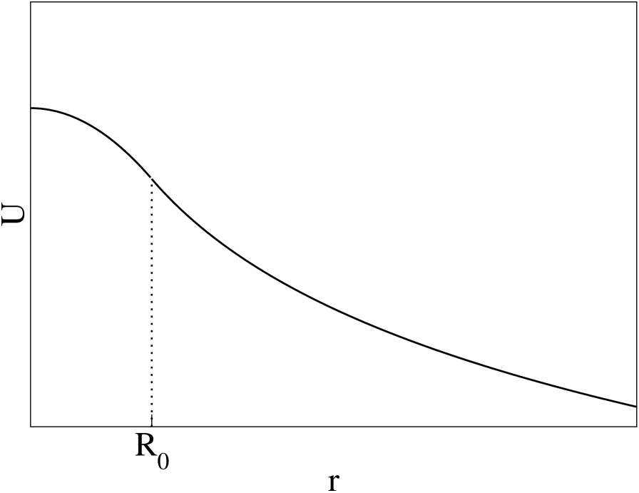
Figure 1: The self-energy of a charged particle in the presence of a disclination density.

The self-force in the outside region is obtained directly from: $\vec{F}=-\vec{\nabla}U$, where $\vec{\nabla}U=e^{(\Omega)}\vec{\nabla_{E}}U$. Thus, in the outside region,

$$\vec{F}_{out}=\frac{Q^{2}qR_{0}^{2}}{8\pi}\frac{r^{qR_{0}^{2}/2}}{r}\hat{e}_{r}.$$ (31)

This result is better understood if we introduce a new radial variable $\rho$ such that

$$\left(1-\frac{qR^{2}_{0}}{2}\right)\rho=r^{\left(1-qR^{2}_{0}/2\right)}.$$ (32)

In this way, the self-force can be written as

$$\vec{F}_{out}=\frac{Q^{2}(qR^{2}_{0}/2)}{4\pi(1-qR^{2}_{0}/2)}\frac{\hat{e}_{r}}{\rho}.$$ (33)

We notice that this self-force is equivalent to the force between two charges of moduli $Q$ and $Q(qR^{2}_{0}/2)/(1-qR^{2}_{0}/2)$. The charges are separated by a distance $\rho$. Inside the defect the particle has the following self-energy

$$U_{in}=\frac{qQ^{2}R^{2}_{0}}{8\pi}\left[\ln(R_{0})+\frac{r^{2}}{2R_{0}^{2}}-\frac{1}{2}\right].$$ (34)

This shows a harmonic behavior for the electrostatic energy inside the defect. The self-force is given by

$$\vec{F}_{in}=-\frac{qQ^{2}R_{0}^{2}}{8\pi}\exp\left[\ln(R_{0})+\frac{r^{2}}{2R_{0}^{2}}-\frac{1}{2}\right]r\hat{e}_{r}.$$ (35)

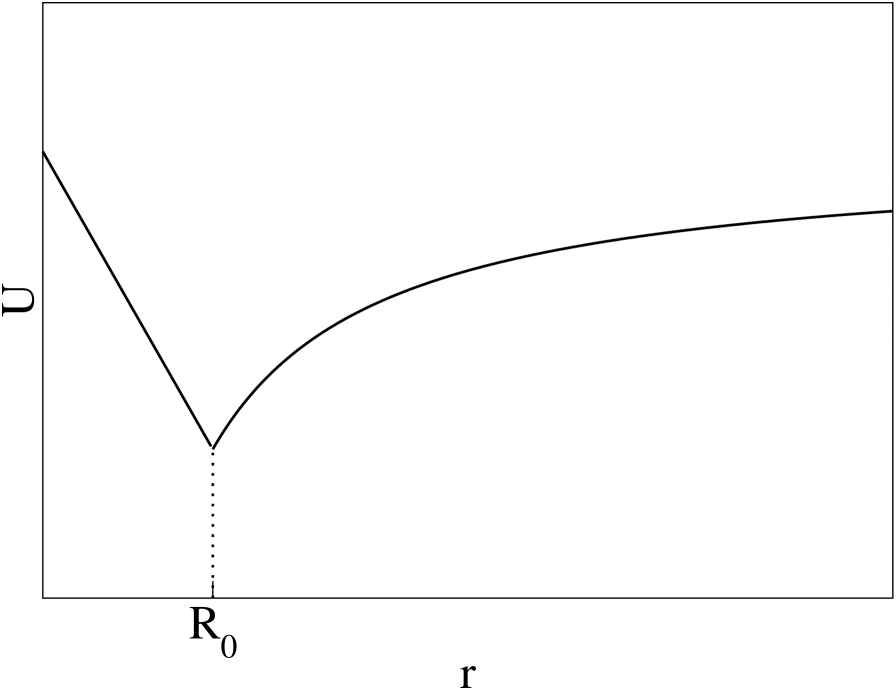
Figure 2: The self-energy of a charged particle in the presence of an edge dislocation density.

Notice the discontinuity of the self-force in the boundary $r=R_{0}$ in spite of the self-energy be continuous. Another interesting behavior of the self-force is that the charge is attracted by the defect density independently of the its sign.

IV.2 The edge dislocation density

In this subsection we determine the self-energy of a punctual charge in the presence of a density distribution of edge dislocations. From (23), (29) and (19),The self-energy in the defect region is given by

$$U_{in}=-\frac{Q^{2}\beta r\cos\theta}{8\pi}.$$ (36)

The behavior of the self-energy, for fixed $\theta$, is shown in figure 2. Notice that the self-energy as a function of $\theta$ can be either positive or negative, meaning attractive or repulsive regions of space. The self-force which acts on the charge can be easily obtained just by taking the negative gradient of the energy

$$\vec{F}_{in}=\frac{Q^{2}\beta}{8\pi}\exp(\beta r\cos\theta/4)\left(-\cos\theta\hat{e}_{r}+\sin\theta\hat{e}_{\theta}\right).$$ (37)

In the outside region the self-energy is

$$U_{out}=-\frac{Q^{2}\beta R_{0}^{2}\cos\theta}{8\pi r},$$ (38)

and the self-force is given by

$$\vec{F}_{out}=\frac{Q^{2}\beta R_{0}^{2}}{8\pi r^{2}}\exp(\beta R_{0}^{2}\cos\theta/4)\left(\cos\theta\hat{e}_{r}+\sin\theta\hat{e}_{\theta}\right).$$ (39)

The expression (38) is in agreement with the previous results obtained by the Potential Deformation Theory pr:bs . This approach was used to find the energy interaction of electrons and holes in a solid that contains a single edge dislocation.

V Concluding Remarks

In this work we determined the self-energy of a single charge in the presence of either a continuous distribution of disclinations or a continuous distribution of dislocations. We used the geometrical theory of defects in solids to describe the defect distributions in an elastic medium. We also have used Grats and Garcia’s method for finding the two-dimensional Green function in a space associated to a conformal metric. This allowed us to determine the self-energy and self-force experimented by the charged particle in the presence of a circular distribution of disclinations. We obtained the self-energy both for the region inside and outside the distribution. We notice that the self-energy is continuous in the boundary between the internal and external regions but the self-force is discontinuous in both cases. The analysis of the behavior of the self-energy shows that in the external region the charge “feels” an effective distribution acting as a single defect in both cases.

Notice that outside the dislocation density region one has a metric which corresponds to an effective dislocation. The self-force due to the distribution should be compared with the results of reference carvalho , where the dipole approximation was used for the metric of a dislocation. Notice also that the sudden change in the metrics from the defect density region ($r<R_{0}$) to the defect-free region ($r>R_{0}$) causes the curve of the self-energy as function of r to change its concavity. In the dislocation case, the effect is even more drastic, besides the change in concavity the derivative (e.g. self-force) goes discontinuous at $r=R_{0}$. Notice also that both in the disclination and in dislocation cases, the self-energy is attractive independently of the signal of the charge $Q$. This gives the possibility of trapping charges in the defect density. In the dislocation case there is an additional asymmetry in the azimuthal angle, creating regions alternatively of attraction and repulsion as one goes around the $z$ axis.

Acknowledgments
We are indebted to Gustavo Camelo for helping with the figures and to Mario Henrique de Oliveira for important discussions. This work was partially supported by CNPq, FINEP (PRONEX) and CAPES (PROCAD).

References

References

- (1) G. E. Volovik, The Universe in a Helium Droplet (Oxford University Press)2003.
- (2) W. G. Unruh, Phys. Rev. D, 51 6(1995).
- (3) L. J. Garay, J. R. Anglin, J. I. Cirac, and P. Zoller Phys. Rev. lett. 85, 4643 (2000).
- (4) L. J. Garay, J. R. Anglin, J. I. Cirac and P. Zoller Phys. Rev. 63 023611 (2001).
- (5) Matt Visser, Class. Quant. Grav. 15 1767 (1998).
- (6) M. Novello, Int. J. Mod. Phys A 17 29, 4187 (2002).
- (7) M. Katanaev and I. Volovich, Annals of Physics 216, 1(1992).
- (8) J. Bardeen and W. Schockley, Phys. Rev. 80, 72 (1950).
- (9) C. Furtado and F. Moraes, Phys Lett. A 188, 394(1994)
- (10) C. Furtado and F. Moraes, Europhys. Lett. 45, 279(1994).
- (11) C. Furtado, V. B. Bezerra and F. Moraes, Europhys. Lett. 52, 1(2000).
- (12) M. Katanaev and I. Volovich, Annals of Physics 272, 203(1999).
-
(13)
C. M. De Witt and B. S. De Witt,
Physics 1 3 (1964)
W. G. Unruh, Proc. R. Soc. London A348, 447 (1976). - (14) A. Vilenkin, Phys. Rev. D 20, 373 (1979).
- (15) B. Linet, Phys. Rev. D 33, 1833 (1986).
- (16) A. G. Smith, in Proceedings of Symposium on The Formation and Evolution of Cosmic String, edited by G. W. Gibbons, S. W. Hawking, and T. Vachaspati(Cambridge Unversity Press, Cambridge , England, 1990).
- (17) T. Souradeep and V. Sahni, Phys. Rev. D 46, 1616 (1992).
- (18) C. Furtado and F. Moraes, Classical Quant. Grav. 14, 12, 3425 (1997).
- (19) M. E. X. Guimaraes and B. Linet , Class. Quantum Grav. 10, 1665 (1993).
- (20) E. R. Bezerra, V. B. Bezerra, C. Furtado and F. Moraes, Phys. Rev. D 51 7140 (1994).
- (21) E. R. B. de Mello and C. Furtado, Phys. Rev. D 56 1345 (1997).
- (22) A. M. de M. Carvalho, C. Furtado and F. Moraes, Phys Rev D 62, 067504 (2000).
- (23) S. Azevedo and F. Moraes, J. Phys. Condens. Matter 12 7421 (2000).
- (24) V. A. de Lorenci and E. S. Moreira Jr, Phys Rev D 65, 085013 (2002).
- (25) N. R. Khusnutdinov and V. B. Bezerra, Phys Rev D 64 083506 (2001)
- (26) F. Moraes, A. M. de M. Carvalho, I.V.L. Costa, F. A. Oliveira and C. Furtado, Phys Rev D 68 043512 (2003).
- (27) H. Kleinert, Gauge fields in Condensed Matter, Vols. I, II (World Scientific, Singapore, 1989).
- (28) A. Holz, Clas. Quant. Grav. 5 1259 (1988).
- (29) R. A. Puntigam, Clas.Quant. Grav. 14 1129(1997).
- (30) C. Kohler, Clas. Quant. Grav. 12 2977(1995).
- (31) R. Bausch , R. Schmitz and L. A. Turski, Phys. Rev. Lett.80 2257 (1998).
- (32) M. O. Katanaev, Theor.Math.Phys. 135 733 (2003).
- (33) Yu Grats and A Garcia, Class. Quantum Grav. 13, 189(1996).
- (34) J D Jackson, Classical Electrodynamics, Wiley and Sons, 2nd edition.
- (35) E R B de Mello, V B Bezerra and Yu Grats, Class. Grav. 13, 1915 (1998)
- (36) E R B de Mello, V B Bezerra and Yu Grats, Modern Physics Lett. A. 13, 1427 (1998)