The Periodic Standing-Wave Approximation: Overview and Three Dimensional Scalar Models

Abstract

Abstract

The periodic standing-wave method for binary inspiral computes the exact numerical solution for periodic binary motion with standing gravitational waves, and uses it as an approximation to slow binary inspiral with outgoing waves. Important features of this method presented here are: (i) the mathematical nature of the “mixed” partial differential equations to be solved, (ii) the meaning of standing waves in the method, (iii) computational difficulties, and (iv) the “effective linearity” that ultimately justifies the approximation. The method is applied to three dimensional nonlinear scalar model problems, and the numerical results are used to demonstrate extraction of the outgoing solution from the standing-wave solution, and the role of effective linearity.

I Introduction

Background

The inspiral and merger of a binary pair of compact objects (holes or neutron stars) is one of the most promising sources of signals detectable by gravitational wave observatories. For the ground-based detectors LIGOgonzalez03 , VIRGOvirgostatus , GEO6002000grwa.conf..119L and TAMAAndo:1999qj , binary merger, especially of intermediate-mass black holesColbert:2002mi is an exciting possibility; for the space-based LISA detectorluml.conf ; lisawebpage , the detection of inspiral/merger of supermassive holes is highly probable, and is one of the primary scientific targets.

The need for theoretical waveforms for the inspiral/merger has driven the effort to find a computational solution for the details of the process, but the difficulty of the task has made this problem also a measure of the usefulness of numerical computation in general relativity. The hope has been that numerical codes evolving initial data can compute the orbital motion using Einstein’s equations and, in the case of neutron stars, using hydrodynamical equations. These evolution codes would have, as an intrinsic feature, the loss of energy by the binary due to outgoing wave energy, and the gradual inspiral due to this loss.

An important reason for the limited progress on this problem is the matter of timescales. Near a black hole, the timescale on which the gravitational field can change is $GM/c^{3}$, where $M$ is the mass of the hole; for a neutron star the timescale is several times longer. The time step in evolution codes is governed by this short timescale. (More precisely, the spatial grid near the compact objects must be smaller than $GM/c^{2}$, and to satisfy the Courant condition, the time step must be no larger than $1/c$ times this grid size.) By contrast, the timescale $\sqrt{r^{3}/GM\;}$, for orbital motion at radius $r$, is much larger than this, and the timescale for the interesting dynamics, the radiation-reaction driven inspiral is much greater yet. The consequence of this incompatibility of timescales is that a very large number of time steps is needed in order to see the physics of interest. And computing a large number of time steps is not yet possible. Instabilitiesscheel_stable ; Yo:2002bm operating at the short timescale prevent the code from giving useful answers about the long timescale.

The origin of the difficulty suggests its cure: an approximation method that avoids the short timescales. Here we describe such a method: a solution for periodic sources and fields. We assume that the compact objects, and their fields, rotate with a constant angular velocity (to be denoted $\Omega$ below.) This approximation will fail of course, in the very latest stages of inspiral merger, when the orbit decays rapidly due to a secular instability or the dynamics of the final merger. But that last stage is, by its very nature, rapid; its timescale is only several times that of the shortest timescale of the problem. This last stage, then, can plausibly be handled by numerical evolution codes. Indeed, evolution codes, especially with perturbation theory handling the final ringdownlaz1 , are already near to doing this. Our goal, then, is a method that can approximate the solution up to the time that numerical evolution codes can take over the task that only they can handle. Our approach is not entirely new; it is similar in underlying motivation to a method introduced by Detweiler and collaboratorsdet ; det2 , but our approach is very different in its details and its implementation. It is also very closely related to the approach being used by Friedman and his collaboratorsfriedman .

Periodic motion and outgoing waves are, of course, impossible in Einstein’s theory, both intuitively and mathematically. For this reason, we will solve for standing waves (to be defined and discussed below) in the gravitational field. Our periodic standing-wave (PSW) approach, then, will be to find exact (numerical) periodic standing-wave solutions of the Einstein field equations and to use these exact solutions as approximations to the physical problem of slow inspiral with outgoing waves.

The most basic ideas behind this periodic standing-wave solution have already been introduced in a previous paperWKP , but the implementation there was applied only to two-dimensional models and was limited in other ways; in particular, that paper did not discuss the general meaning of standing waves. An general overview of the PSW project has also been givensafari . Here we present a more specific discussion, along with numerical results for three-dimensional models. This paper is meant to serve as the introduction to the PSW, with subsequent papers presenting more detailed information on particular methods, and progress on solving the physical problem.

Effective linearity and uses of the method

A key idea in our approach is the relationship of standing waves to outgoing waves. In a linear field theory, a definition of standing waves is that they are half the sum of an outgoing solution and ingoing solution. Here, as in Ref. WKP , we shall call this sum LSIO for linear superposition of (half) ingoing and (half) outgoing solutions. In a linear theory, such a superposition is itself a solution. In our nonlinear field model theories, it will turn out that — despite strong nonlinearities — this continues to be very nearly true. This effective linearity, the approximate equality of the LSIO and a true standing-wave solution, has already been demonstrated for simple two-dimensional models, and results for three dimensional nonlinear models will be presented below. More important, the basis for effective linearity appears to be robust. This basis lies in the fact that the strong nonlinearities in our model theories (and in the physical problem) are confined to the near-field regions around the sources. In these nonlinear near-field regions the solution is insensitive to the distant boundary conditions; it is substantially the same for ingoing boundary conditions as for outgoing. In this near-field region then, the LSIO will be very nearly a solution despite strong nonlinearities, since we are superposing nearly identical solutions. Outside this strong-field near zone the model theories, and the physical theory, are nearly linear, so that again the LSIO is a solution. The LSIO will therefore be a good approximation to a solution everywhere.

Below, we shall choose our definitions of standing-wave solution to be close to that of a LSIO, and our approximation to a large extent is based on interpreting a standing-wave solution to be approximately a LSIO. In the weak field region this LSIO can be deconstructed into outgoing and ingoing pieces and this deconstruction can be continued to the strong field source region. (In the source region, the outgoing piece is simply half the solution.) By doubling the outgoing piece thus extracted from the standing-wave solution, we thereby arrive at an approximation to the outgoing solution for a nonlinear problem. It is in this manner that we will extract an approximation of an outgoing solution from a computed standing-wave solution.

This is an appropriate place to point out, though not for the last time, the importance of model problems. In Einstein’s theory there is no obvious meaning to the periodic outgoing solution, so one cannot make statements about it, let alone carry out numerical studies. Statements and computations are possible for nonlinear model problems, so that tests of effective linearity with such models are crucial.

The outgoing solutions extracted from our exact periodic solutions can serve two purposes. First, we can use a quasistationary sequence of outgoing approximations as a model for the slow physical inspiral. In this approach the mass of the system, measured in a weak wave zone far from the orbiting sources, decreases due to the loss of energy in outgoing radiation. When we find the system energy as a function of orbit radius, and we compute the outgoing radiation, we can infer the rate at which the orbital radius decreases. The difficulty, as with any such quasistationary sequence, is how to know that we are comparing the “same” system at different radii. In the case of neutron star’s the answer is clear; baryon number is an unchanging tag that identifies neutron stars to be the same. For black holes, the equivalent tag would be some local mass. The concept of an isolated horizonAshtekar:2000sz might give us that local mass.

The second use for our extracted outgoing solutions is to provide initial data for evolution codes. A spacelike slice of our extracted outgoing field will be an excellent approximation to the physical initial data, and should be very nearly a solution to the initial value equations. With little change our extracted outgoing initial data, can be made into exact (numerical) initial data through the use of York’s decompositionYork71 ; York73 .

These two purposes of our solution are not distinct. The natural end point for a quasistationary sequence of PSW solutions is the “last orbit,” the final stage of motion at almost constant radius. This stage may end due to a secular instability, like that of a particle in a black hole spacetime, or due to the imminence of the merger, the formation of the final black hole. In either case, this end point must be handled by a numerical evolution code, and in either case, the quasistationary sequence will provide ideal initial data for the continuation of the problem by numerical evolution.

The nature of the mathematical problem

In the standard approach to computing binary inspiral, initial data are evolved forward in time. In our approach, with periodic symmetry imposed, there is no evolution in the usual sense, and there is not the usual concept of initial data. Rather we must satisfy boundary conditions at large radius: outgoing, ingoing or standing-wave boundary conditions in model problems, and only standing-wave conditions in general relativity. The boundary value problems that we must solve differ in two important ways from common boundary value problems. First, our partial differential equations (PDEs) are of mixed type. They are of elliptical character in some regions and hyperbolic character in others; this will be particularly clear in the model problem to be presented below. We will argue that the mixed character causes no fundamental difficulty, and will demonstrate this with the model problems. The mixed character, however, does complicate the use of some of the most efficient numerical means of solving bounary value problems. Second, we must define what we mean by “standing-wave boundary conditions.” Unlike outgoing and ingoing conditions, there is no simple local condition corresponding to what we will mean by standing waves in a nonlinear problem. We will present two fundamentally different candidates for the standing-wave condition, and here will present results of computations with one those of those two choices. (The alternative choice of standing-wave condition is best implemented with a special numerical method, and will be presented elsewherepaperII .)

Stepping back from such details, one may be led to ask more fundamental questions about the whole approach. Such questions arise especially because the PSW spacetime we compute has some awkward features. Since the exact PSW solution contains an infinite amount of gravitational wave radiation, it cannot be expected to be meet the asymptotic flatness conditions of the theorems about the fall-off of fields. But the spacetime is asymptotically flat in that the spacetime curvature decreases with increasing distance from the binary source. Another sign that the PSW spacetime has rough edges is that it must not have regular null infinities; Gibbons and StewartGibbonsStewart have shown that spacetimes with well-behaved Scri+ and Scri– cannot be periodic.

It is useful, before diving into details, to clarify what the relationship is between the slightly singular spacetime we will be computing, and the physical problem that really interests us. To make this connection we can think of the binary system going through several orbits at almost constant radius. A weak wave zone exists at some distance from the orbit during this epoch of the motion. The stippled region in Fig. 1 shows the relevant region as part of the larger physical spacetime. In this limited region the source motion and the fields are almost periodic, and it is in this region only that we hope to approximate the physical fields by the outgoing fields extracted from the computed PSW solution. The imperfect asymptotic structure of the PSW spacetime is therefore irrelevant to its physical usefulness.

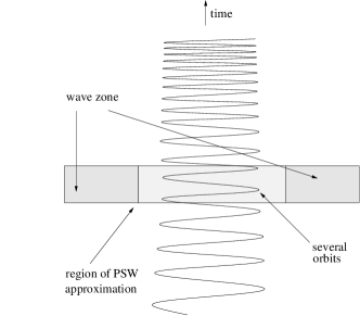
Figure 1: The PSW solution is meant to be an approximation to the physical spacetime only in a limited region.

In the remainder of this paper we will first present, in Sec. II, the mathematical details of a nonlinear model with which we clarify many aspects of the PSW approximation. We then discuss, in Sec. III, the numerical methods needed to find PSW solutions, especially those aspects of the numerical methods that are idiosyncratic to the special features (mixed character, standing-wave boundary conditions, nonlinearities) of our problem. In this section also, results are presented of the numerical methods. The results are discussed, and put into the context of the next steps in this projectpaperII , in Sec. IV.

II Periodic solutions, standing waves, and model problems

Mixed PDEs and well-posedness

As stated above, we seek a solution to Einstein’s equations in which the sources and the fields rotate rigidly. The mathematical statement of this rigid rotation is that there is a helical Killing vector, a Killing vector that is timelike close to the sources and spacelike far from the sources. (For more on helical Killing symmetry see Ref. friedmanuryushibata .) For fields in flat spacetime our Killing vector $\vec{\xi}$ takes the form

$$\vec{\xi}=\partial_{t}+\Omega\partial_{\phi}$$ (1)

in spherical or cylindrical spatial coordinates, and

$$\vec{\xi}=\partial_{t}+\Omega\left(x\partial_{y}-y\partial_{x}\right)$$ (2)

in Cartesian spatial coordinates. The parameter $\Omega$, which must be a constant, can be thought of as the rotation rate of the source and fields with respect to an inertial reference frame. For the flat spacetime case, the null surface $\vec{\xi}\cdot\vec{\xi}=0$ is a cylinder of radius $1/\Omega$ coaxial with the rotation axis. (Here and below we use units in which $G=c=1$.) This cylinder separates the inner region of timelike $\vec{\xi}$ from the outer region of spacelike $\vec{\xi}$, as shown in Fig. 2. Since this surface, in a sense, represents the points at which the rigidly rotating fields are moving at $c$, we call this surface the “light cylinder,” in analogy with pulsar electrodynamics.

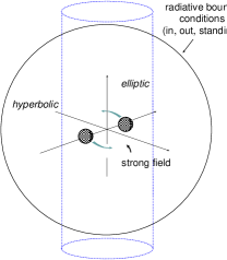
Figure 2: The “light cylinder” separating the elliptic and hyperbolic regions of the problem intersects the large spherical surface on which numerical boundary conditions are imposed.

One immediate advantage of the helical symmetry is that it reduces the number of independent variables, thereby greatly reducing the computational difficulty of a problem. In our simple flat spacetime models this reduction is most easily understood by the fact that helically symmetric scalars cannot depend in an arbitrary way on the spherical Minkowski coordinates $t,r,\theta,\phi$ but can depend only on $t$ and $\phi$ in the combination $\varphi\equiv\phi-\Omega t$. Thus, in the $t,r,\theta,\varphi$ system the Killing vector is $\vec{\xi}=\partial_{t}$. These ideas are clarified with a simple flat spacetime model theory for a scalar field $\Psi$

$$\Psi_{;\alpha;\beta}g^{\alpha\beta}+\lambda F=S\;.$$ (3)

The term $F(\Psi,x^{\alpha})$ is included to allow for nonlinearity; the constant $\lambda$ adjusts the strength of the nonlinearity. In order for a helically symmetric solution $\Psi$ to exist, the explicit coordinate dependence of $F$ must be compatible with the symmetry. That is, $F$ can have explicit coordinate dependence only on $r$, $\theta$, and $\varphi$. The most natural choice for a model would be one in which there is no coordinate dependence, one in which the background spacetime is featureless. We include the possibility of spatial dependence for convenience below. Changing the spatial dependence will help to clarify the accuracy of the PSW approximation when nonlinearities are important.

In the application of the PSW method to holes, an inner boundary condition will be used at a small, approximately spherical surface. For simplicity here, however, we use an explicit source term,

$$S=\frac{\delta(r-a)}{a^{2}}\;\delta(\theta-\pi/2)\left[\delta(\varphi)+\delta(\varphi-\pi)\right]\,,$$ (4)

representing two points, each of unit scalar charge, in equatorial circular orbits, with radius $a$ and angular velocity $\Omega$. This source term $S$ obeys the symmetry property that is necessary if a periodic solution is to exist: its Lie derivative vanishes along the Killing orbit ${\vec{\xi}}$.

If we are interested only in helically symmetric solutions, then the field equation (3) reduces to

$$\frac{1}{r^{2}}\frac{\partial}{\partial r}\left(r^{2}\frac{\partial\Psi}{\partial r}\right)+\frac{1}{r^{2}\sin\theta}\frac{\partial}{\partial\theta}\left(\sin\theta\frac{\partial\Psi}{\partial\theta}\right)+\left[\frac{1}{r^{2}\sin^{2}\theta}-\Omega^{2}\right]\,\frac{\partial^{2}\Psi}{\partial\varphi^{2}}+\lambda F(\Psi,r,\theta,\varphi)=S(r,\theta,\varphi)\ .$$ (5)

The mixed character of this PDE shows clearly in the coefficient of $\partial_{\varphi}^{2}\Phi$. The light cylinder is at $r\sin\theta=1/\Omega$ where this coefficient changes sign. Inside the light cylinder ($r\sin\theta<1/\Omega$) the equation is elliptical; outside it is hyperbolic. For outgoing solutions of this equation we impose an outer boundary condition $\partial_{r}\Psi=-\partial_{t}\Psi$, or equivalently $\partial_{r}\Psi=\Omega\partial_{\varphi}\Psi$, on a spherical surface with a radius large compared to $1/\Omega$. As illustrated in Fig. 2, this spherical surface is well outside the light cylinder in the equatorial plane, so our boundary conditions are imposed on a surface that passes through both the elliptic and hyperbolic regions of the problem.

Problems with boundary conditions on closed surfaces are common in the case of elliptical PDEs. We argue here that our boundary value problem with mixed PDEs may be unusual, but is well posedctorre . Again, a simple model problem will help to clarify issues. We set the nonlinearity parameter $\lambda$ to zero in Eq. (5) so that we can solve the resulting linear equation as an infinite series. If we choose a Dirichlet condition

$$\left.\Psi\right|_{r=r_{\rm max}}=0\,,$$ (6)

at a finite radius $r_{\rm max}$, then the solution to this linear problem can be written in terms of spherical Bessel functions $j_{\ell},n_{\ell}$ as

$$\Psi=\sum_{\ell}\sum_{m={\rm even}}\frac{2m\Omega Y^{*}_{\ell m}(\pi/2,0)Y_{\ell m}(\theta,\varphi)}{j_{\ell}(m\Omega r_{\rm max})}j_{\ell}(m\Omega r_{<})\left[n_{\ell}(m\Omega r_{>})j_{\ell}(m\Omega r_{\rm max})-n_{\ell}(m\Omega r_{\rm max})j_{\ell}(m\Omega r_{>})\right]\ .$$ (7)

Here $r_{<}(r_{>})$ indicates the smaller (greater) of the quantities $r,a$. Vanishing of the $j_{\ell}(m\Omega r_{\rm max})$ denominator means that the the “cavity” $r\leq r_{\rm max}$ has a resonant mode at frequency $\Omega$. In the case that $r_{\rm max}$ has one of the resonant values, the solution to the boundary value problem is not unique. Such values of $r$ are of zero measure, but are dense in the set of all $r$ choices. This means that the cavity is always arbitrarily close to a resonance, if sufficiently high angular modes are computed. A consequence of this is that a numerical computation does not converge. (Computed solutions depend on the computational grid size, and become larger with increasing angular resolution.) The difficulty is not just one of computational practice. The boundary value problem is fundamentally ill-posed as a representation of fields in an infinite space. There is no meaningful $r_{\rm max}\rightarrow\infty$ limit of Eq. (7).

Problems with mixed elliptic and hyperbolic regions are of some interest in aerodynamicstricomi , but there are few general results on well-posedness. In those results that do exist, the nature of the boundary conditions plays a pivotal role. We have found that this applies to our periodic solutions also. If we replace the Dirichlet conditions of Eq. (7) with the Sommerfeld condition

$$\left(\partial_{r}\Psi-\Omega\partial_{\varphi}\Psi\right)_{r=r_{\rm max}}=0\,,$$ (8)

then the problem is found to be well-posed. This is particularly clear for the linear problem, where the closed form solution takes the form

$$\Psi=\Psi_{\rm out}+\Psi_{\rm extra}\ .$$ (9)

Here $\Psi_{\rm out}$ is the usual “outgoing at infinity” solution

$$\Psi_{\rm out}=\sum_{\ell}\sum_{m={\rm even}}{-2im\Omega Y^{*}_{\ell m}(\pi/2,0)Y_{\ell m}(\theta,\varphi)}j_{\ell}(m\Omega r_{<})h^{(1)}_{\ell}(m\Omega r_{>})$$ (10)

and

$$\Psi_{\rm extra}\equiv\sum_{\ell}\sum_{m={\rm even}}{-2im\Omega Y^{*}_{\ell m}(\pi/2,0)Y_{\ell m}(\theta,\varphi)}\;\gamma_{\ell m}\;j_{\ell}(m\Omega r_{<})j_{\ell}(m\Omega r_{>})$$ (11)

with

$$\gamma_{\ell m}\equiv-\left(\;\frac{h_{\ell}^{(1)}(z)+i\,dh_{\ell}^{(1)}(z)/dz}{j_{\ell}(z)+i\,dj_{\ell}(z)/dz}\right)_{z=m\Omega r_{\rm max}}\ .$$ (12)

Since the spherical Hankel function has the asymptotic form $h^{(1)}_{\ell}(z)=(-i)^{(\ell+1)}e^{iz}[1/z+{\cal O}(1/z^{2})]$, it follows that $|\gamma_{\ell m}|$ is of order $1/r_{\rm max}$. Thus, $\Psi\rightarrow\Psi_{\rm out}$, as $r_{\rm max}\rightarrow\infty$, suggesting that the linear problem is well posedprev .

Numerical results confirm this suggestion. With the boundary condition in Eq. (8), we have encountered no fundamental difficulty computing convergent solutions to both the linear and nonlinear versions of Eq. (5), and have confirmed that solutions do not depend on the particular (large) value chosen for $r_{\rm max}$.

Standing waves: iterative method

The solutions we will be computing in Einstein’s theory, of course, are standing wave solutions, but there are no actual “standing wave boundary conditions” analogous to the Sommerfeld condition in Eq. (8) for outgoing waves. It is useful, therefore, to explore the meaning of standing-wave solutions with our model nonlinear theories. As pointed out in Sec. I, our paradigm for standing waves is the LSIO of a linear theory, the linear superposition of half ingoing and half outgoing solutions. We shall extend this definition of standing wave to nonlinear theories in two ways. The first is an extension of the Green function method of Ref. WKP , and is called there the TSGF (time symmetric Green function) method. For the problem in Eq. (3) this method starts by writing the field equation in the form

$${\cal L}[\Psi](\Psi)=\sigma_{\rm eff}[\Psi]\,.$$ (13)

Here the operator ${\cal L}[\Psi]$ depends on $\Psi$ but — once $\Psi$ is fixed — can be considered to be linearly operating on $\Psi$. Similarly $\sigma_{\rm eff}$ depends on $\Psi$, but — once $\Psi$ is fixed— is to be considered a fixed inhomogeneous term in the equation, an effective source term. There is no unique way of putting the field equation into the form of Eq. (13) for a nonlinear model problem, or for general relativity. The quasilinearity of general relativity, and of our nonlinear models, means that at least the principal part of ${\cal L}$ is always unambiguous. There are also some obvious guidelines to follow. In particular, ${\cal L}$ and $\sigma_{\rm eff}$ should become $\Psi$-independent in the weak field limit.

To iterate for an outgoing solution, for example, one would find an approximate outgoing solution $\Psi^{n}_{\rm out}$, and then would solve

$${\cal L}[\Psi^{n}_{\rm out}](\Psi^{n+1}_{\rm out})=\sigma_{\rm eff}[\Psi^{n}_{\rm out}]\,,$$ (14)

for outgoing boundary conditions. The result would be the improved approximation $\Psi^{n+1}_{\rm out}$ to the outgoing waves. To find standing waves, this method is modified as follows. An approximation $\Psi^{n}_{\rm stnd}$ is found to the standing-wave solution. The equation

$${\cal L}[\Psi^{n}_{\rm stnd}](\Psi^{n+1})=\sigma_{\rm eff}[\Psi^{n}_{\rm stnd}]\,,$$ (15)

is then solved with the outgoing boundary conditions of Eq. (8) to give $\Psi^{n+1}_{\rm stout}$ and is next solved with ingoing boundary conditions $\Omega\rightarrow-\Omega$ in Eq. (8)] to give $\Psi^{n+1}_{\rm stin}$. The new approximation for the standing-wave solution is taken to be

$$\Psi^{n+1}_{\rm stnd}=\textstyle{\frac{1}{2}}\,\Psi^{n+1}_{\rm stout}+\textstyle{\frac{1}{2}}\,\Psi^{n+1}_{\rm stin}\ .$$ (16)

We take the $n\rightarrow\infty$ limit of $\Psi^{n+1}_{\rm stnd}$ in Eq. (16) to be our computed standing-wave solution.

We shall call the iterative method just described “direct iteration.” This sort of direct iteration is useful in solving for the root of an equation $x=f(x)$ only if $f$ is slowly varying. In iteration for $\Psi$ the equivalent condition applies to ${\cal L}^{-1}\circ\sigma_{\rm eff}$, where ${\cal L}^{-1}$ is the Green function, the inverse of ${\cal L}$ for the boundary conditions (ingoing or outgoing) of interest. For direct iteration to converge the dependence of ${\cal L}^{-1}\circ\sigma_{\rm eff}$ on $\Psi$ must be weak and this is the case only for nonlinearities of moderate strength. For strong nonlinearities another technique must be used.

In Newton-Raphson iteration, one uses the iteration $\Psi^{n}$ to make linear approximations for ${\cal L}$ and $\sigma_{\rm eff}$. Equation (13) then takes the form

$${\cal L}[\Psi^{n}](\Psi)+(\Psi-\Psi^{n})\times\left[\frac{\partial{\cal L}[\Psi]}{\partial\Psi}\right]_{\Psi=\Psi^{n}}(\Psi^{n})=\sigma_{\rm eff}[\Psi^{n}]+(\Psi-\Psi^{n})\times\left[\frac{\partial\sigma_{\rm eff}}{\partial\Psi}\right]_{\Psi=\Psi^{n}}\ .$$ (17)

This equation is linear in $\Psi$, and its solution is taken to be the next iteration $\Psi^{n+1}$. By choosing appropriate boundary conditions we can use this scheme to iterate an outgoing or ingoing solutions. For our standing-wave solution, we follow the same general scheme as with direct iteration. Using the $n^{\rm th}$ standing-wave approximation as $\Psi^{n}$ in Eq. (17) we solve using both in- and outgoing boundary conditions. As in Eq. (16), the $n+1^{\rm th}$ standing-wave approximation is taken to be half the sum of the ingoing and outgoing solutions found this way.

Standing waves: minimization method

To explain our second, independent way of defining and computing standing-wave solutions, it is best to start with the standing-wave solution in the linear model problem. This is simply half the sum of the “outgoing at infinity” solution in Eq. (10), and the equivalent ingoing solution. The result is

$$\Psi_{\rm stnd}=\sum_{\ell}\sum_{m={\rm even}}{2m\Omega Y^{*}_{\ell m}(\pi/2,0)Y_{\ell m}(\theta,\varphi)}j_{\ell}(m\Omega r_{<})n_{\ell}(m\Omega r_{>})\ .$$ (18)

In this solution each multipole has an equal amplitude for ingoing and outgoing amplitudes waves, and one might suspect that this property suffices to define standing waves for a nonlinear model. This is not, in fact the case, since we could add a multiple of the homogeneous solution $j_{\ell}(m\Omega r)j_{\ell}(m\Omega a)$ to the $\ell,m$ mode without changing the balance between ingoing and outgoing. This degree of freedom is equivalent to the degree of freedom inherent in the phase between the outgoing and ingoing waves. This extra degree of freedom exists also (though not so transparently) in a nonlinear problem.

To resolve this degree of freedom we can use a generalization of a property that is unique, in the linear case, to the correct standing-wave solution Eq. (18): In each multipole, the solution is required to have the minimum wave amplitude of any solution with balanced ingoing and outgoing wavesWBLandP .

This method, while very interesting in principle, is difficult in practice to implement in a finite difference boundary value approach. One could imagine using a guess for the value of a multipole coefficient at some outer boundary, and then searching for the value that gives the minimum for the amplitudes of the waves in that multipole. In a nonlinear problem, the values of each multipole will influence other multipoles, so the search for minimum waves will, in principle, be a search in a many dimensional space.

The real difficulty of this numerical approach is that it uses multipoles as part of the boundary condition. That means that multipole coefficients must be extracted. Even in spherical coordinates, the extraction of the multipole coefficients involves a weighted sum over all angular grid points. Most important, this sum would not be performed as a postprocessing step on a computed solution, but rather would have to be written as a set of equations that would form part of the a priori problem to be solved. The set of equations to be solved would then have, in addition to great complexity, a boundary-related subset connecting distant grid points. The matrix representation of these equations would not have banded structure. In addition to these technical difficulties, the use of spherical coordinates is very ill suited to the structure of our source objects, so coordinate patches for the sources would be required.

For these reasons, we have not attempted to use the minimization criterion in a finite difference code. We have, however, implemented this criterion with a spectral approach based on a specially adapted coordinate system. Results from this approach are extremely encouraging, but the approach poses new computational challenges, so we are continuing to explore two distinct paths: finite difference methods and the iterative definition of standing waves, and a spectral/adapted coordinate technique for the minimization criterion. Since the adapted coordinate system necessary for the second approach requires a separate development, and is not fundamental to the PSW approximation, we confine the present discussion to the first approach, finite difference boundary value problems, with the iterative criterion for standing waves.

III Numerical implementation and results

Extraction of an outgoing approximation

Model problems allow us to test a key idea of the PSW approach, that a good approximation of the outgoing solution can be extracted from the computed standing-wave solution

$$\Psi_{\rm stndcomp}=\sum_{\mbox{even $\ell$}}\ \ \sum_{m=0,\pm 2,\pm 4..}\alpha_{\ell m}(r)Y_{\ell m}(\theta,\varphi)\,.$$ (19)

The coefficients $\alpha_{\ell m}(r)$ are computed from $\Psi_{\rm comp}$, by projection with $Y^{*}_{\ell m}$. From the reality of $\Psi_{\rm stndcomp}$, the coefficients will obey $\alpha_{\ell m}^{*}=\alpha_{\ell-m}$, and from the standing-wave symmetry ($\cos{m\varphi}$ only, no $\sin{m\varphi}$ terms) they will also obey $\alpha_{\ell m}=\alpha_{\ell-m}$.

This form of the computed standing-wave solution is compared with a general homogeneous linear ($\lambda=0$) standing-wave (equal magnitude in- and outgoing waves) solution of Eq. (5), with the symmetry of two equal and opposite sources:

$$\Psi_{\rm stndlin}=\sum_{\mbox{even $\ell$}}\ \ \sum_{m=0,\pm 2,\pm 4..}Y_{\ell m}(\theta,\varphi)\,\left[\textstyle{\frac{1}{2}}\;C_{\ell m}h^{(1)}_{\ell}(m\Omega r)+\textstyle{\frac{1}{2}}\;C^{*}_{\ell m}h^{(2)}_{\ell}(m\Omega r)\right]\,,$$ (20)

where $C_{\ell-m}=C_{\ell m}^{*}$, from the reality of $\Psi_{\rm stndlin}$. A fitting, in the weak-field zone, of this form of the standing-wave multipole to the computed function $\alpha_{\ell m}(r)$ gives the value of $C_{\ell m}$.

By viewing the linear solution as half-ingoing and half-outgoing we define the extracted outgoing solution to be

$$\Psi_{\rm exout}=\sum_{\mbox{even $\ell$}}\ \ \sum_{m=0,\pm 2,\pm 4..}Y_{\ell m}(\theta,\varphi)\,C_{\ell m}h^{(1)}_{\ell}(m\Omega r)\ .$$ (21)

Since this extracted solution was fitted to the computed solution assuming only that linearity applied, it will be a good approximation except in the strong-field region. In the problems of interest, the strong-fields should be confined to a region near the sources. In those regions, small compared to a wavelength, the field will essentially be that of a static source, and will be insensitive to the distant radiative boundary conditions. As pointed out in Sec. I, the solutions in this region will be essentially the same for the ingoing, outgoing, and standing-wave problem. In this inner region then, we take our extracted outgoing solution simply to be the computed standing-wave solution, so that

$$\Psi_{\rm exout}=\left\{\begin{array}[]{ll}\sum Y_{\ell m}C_{\ell m}h^{(1)}_{\ell}&\mbox{weak field outer region}\\ \Psi_{\rm stndcomp}&\mbox{strong field inner region}\end{array}\right.\ .$$ (22)

The boundary between a strong field inner region and weak field outer region would ideally be a closed surface surrounding each of the source regions. This is easily implemented with the adapted coordinates to be introduced in a subsequent paper. Here, for simplicity, we take the boundary to be a spherical surface around the origin. In order for the extracted solution to be smooth at this boundary, we use a blending of the inner and outer solution in a transition region extending between radii $r_{\rm low}$ and $r_{\rm high}$ and, in this region, we take

$$\Psi_{\rm exout}=\beta(r)\;\sum Y_{\ell m}C_{\ell m}h^{(1)}_{\ell}+[1-\beta(r)]\;\Psi_{\rm stndcomp}\,.$$ (23)

Here

$$\beta(r)\equiv 3\left[\frac{r-r_{\rm low}}{r_{\rm high}-r_{\rm low}}\right]^{2}-2\left[\frac{r-r_{\rm low}}{r_{\rm high}-r_{\rm low}}\right]^{3}\,,$$ (24)

so that $\beta(r)$ goes from 0 at $r=r_{\rm low}$ to unity at $r=r_{\rm high}$ and has a vanishing $r$-derivative at both ends.

In the case of our typical choice $\Omega=0.3$, the value of $r_{\rm low}$ is chosen to be $r=1.3\,a$ the value at which the static and standing-wave solutions of the linear problem differ by 10%. This value should decrease with increasing $\Omega$, but it must be larger than the orbital radius $r=a$, so we choose it to be

$$r_{\rm low}=a[1+0.3(0.3/\Omega)]\,.$$ (25)

In order to have a moderately thin transition region we somewhat arbitrarily take

$$r_{\rm high}=a[1+0.6(0.3/\Omega)]\,.$$ (26)

For the numerical results reported below, the extraction details of Eqs. (19)–(26) are used, and extraction is carried out using the $\ell=0,2,4$ multipoles.

Choice of model

To verify and demonstrate several innovative features (well-posed mixed boundary value problem, standing waves, effective linearity) of the PSW approximation, we use the nonlinear scalar model of Eq. (5), with the $\delta$ function sources given by Eq. (4). We make the simplifying assumption that the nonlinear function $F$ in Eq. (5) depends only on $\Psi$, not on its derivatives. From this an obvious simplification follows for the iteration method of Eqs. (13) – (16). We replace Eq. (13) by

$${\cal L}(\Psi)=\sigma_{\rm eff}[\Psi]\,.$$ (27)

with ${\cal L}$ taken to be

$${\cal L}\equiv\frac{1}{r^{2}}\frac{\partial}{\partial r}\left(r^{2}\frac{\partial}{\partial r}\right)+\frac{1}{r^{2}\sin\theta}\frac{\partial}{\partial\theta}\left(\sin\theta\frac{\partial}{\partial\theta}\right)+\left[\frac{1}{r^{2}\sin^{2}\theta}-\Omega^{2}\right]\,\frac{\partial^{2}}{\partial\varphi^{2}}\,.$$ (28)

The effective source term includes both the true point source and the nonlinear term

$$\sigma_{\rm eff}[\Psi]=\;\frac{\delta(r-a)}{a^{2}}\delta(\theta-\pi/2)\left[\delta(\varphi)+\delta(\varphi-\pi)\right]-\lambda F\,.$$ (29)

Our choice of the nonlinearity function $F$ is

$$F=\frac{\Psi^{5}}{\Psi_{0}^{4}+\Psi^{4}}\,.$$ (30)

(We will comment below on the difference between this choice and that made in previous work, including previous versions of this paper.) Here $\Psi_{0}$ is a second nonlinearity parameter ($\lambda$ being the first). We shall choose $\Psi_{0}$ to be less than unity; in the numerical results to be presented, $\Psi_{0}$ is taken to be $0.15$.

To understand the effect of this nonlinearity, let $R$ denote the distance from one of the point sources. Very near a source point, at very small $R$, where the field is strong, $F$ has the limit $F\rightarrow\Psi$, so that the solution of Eqs. (27)–(30) approximately has the Yukawa form

$$\Psi\approx\frac{e^{-\sqrt{-\lambda\;}R}}{4\pi R}\quad\quad\quad\mbox{\rm near source pt}\,.$$ (31)

At some distance from the source — call it $R_{\rm lin}$ — the field $\Psi$ becomes smaller than $\Psi_{0}$, and $F$ can be approximated as $\Psi^{5}$. Since $\Psi$ itself is less than $\Psi_{0}$, and hence less than unity, this $\Psi^{5}$ nonlinearity is small enough to be considered a perturbative correction.

If the transition at $R_{\rm lin}$ takes place well inside the near zone of the problem, then the effect of the nonlinearity can be understood as follows: Near a source point the solution has the form of a unit strength Yukawa potential. At distance $R_{\rm lin}$ the effect of the $\lambda F$ term is turned off and the solution becomes a simple Coulomb potential. The source strength for this Coulomb field, though, will be less than unity. Due to the $\exp{(-\sqrt{-\lambda}R)}$ Yukawa factor, the source strength decreases in the region from $R=0$ to $R=R_{\rm lin}$, and the effect of the nonlinearity is to reduce the effective source strength by a factor of order $\exp{(-\sqrt{-\lambda}R_{\rm lin})}$. Since this transition takes place well within the near zone, it should be this reduced source strength that is responsible for generating radiation. The effect of the nonlinearity on radiation, then, will be the same reduction factor $\exp{(-\sqrt{-\lambda}R_{\rm lin})}$, and we can easily estimate the size of this nonlinear effect. One estimate can be found by solving

$$\Psi\approx\frac{e^{-\sqrt{-\lambda\;}R_{\rm lin}}}{4\pi R_{\rm lin}}=\Psi_{0}$$ (32)

for $R_{\rm lin}$, and using this value of $R_{\rm lin}$ in the expression $\exp{(-\sqrt{-\lambda}R_{\rm lin})}$ for the reduction factor. Another estimate follows by solving the spherically symmetric static nonlinear problem for a unit strength source

$$\frac{1}{r^{2}}\frac{\partial}{\partial r}\left(r^{2}\frac{\partial\Psi}{\partial r}\right)+\lambda\;\frac{\Psi^{5}}{\Psi_{0}^{4}+\Psi^{4}}=\delta^{3}({\vec{r}})\,.$$ (33)

(Here the right hand side is the unit $\delta$ function at the origin.) For this solution the ratio is found of the large-$r$ monopole moment to the small-$r$ monopole moment, and this ratio is taken as the reduction factor. Since these methods for the reduction factor ignore the nonlinear interaction between the two source points, and since they assume that all the wave generation occurs far outside $R_{\rm lin}$, they can only be considered an approximation for the nonlinear reduction effect on the wave amplitude. We shall see, however, that these estimates are accurate enough to be taken as a good heuristic explanation of the role of the nonlinearity.

In previous work, a form of the nonlinearity was used that was different from that in Eq. (30). To give that previous form we first defined the distance $R_{+}$ ($R_{-}$) from the source point on the $x$ axis at $x=a$ ($x=-a$) to be given by

$$R_{\pm}^{2}=(r\sin\theta\cos\varphi\mp a)^{2}+r^{2}\sin^{2}\!\theta\cos^{2}\!\varphi+r^{2}\cos^{2}\!\theta\,.$$ (34)

We then introduced the distance variable

$$\chi\equiv\sqrt{R_{+}R_{-}\;}\,.$$ (35)

At either of the source points $\chi\rightarrow 0$, and far from the sources $\chi\rightarrow r$. In terms of $\chi$, the form of the nonlinearity previously usedearlierF is

$$F_{\rm prev}=\left(\frac{\chi}{na}\right)^{n}e^{(n-\chi/a)}\;\frac{\Psi^{3}}{1+\Psi^{2}}\,.$$ (36)

The $\chi$-dependent prefactor $(\chi/na)^{n}e^{(n-\chi/a)}$ was included so that we could force the nonlinearity to be concentrated near $\chi=na$. By choosing $n$ to be 5 or 10 we could, in this way, have strong nonlinearity in the wave zone, and we could numerically demonstrate the failure of effective nonlinearity. The $\chi$-dependent prefactor, however, makes it difficult to find a numerical solution that is physically meaningful.

The prefactor is a difficulty because the solution near the source can have either the Yukawa form $\exp{(-\sqrt{-\lambda}R)}$, or the “anti-Yukawa” form $\exp{(+\sqrt{-\lambda}R)}$. If there is any of the latter included in the solution, then the field gets larger at larger distances from the sources, so the strong nonlinearity is never suppressed, the $\lambda F$ term continues to approximate $\lambda\Psi$, and the sum of the Yukawa and anti-Yukawa forms continues to be a valid solution. But if the anti-Yukawa part is present, the solution cannot meet the fall-off conditions at an outer boundary at large $r$. Without the prefactor, then, the outer boundary conditions act to suppress the anti-Yukawa part of a solution. With the prefactor present, however, the nonlinearity can be turned off by the fall off of $\exp{(-\chi/a)}$, even if the solution contains an anti-Yukawa part close to the sources. The prefactor, in effect, shields the inner region from the influence of the outer boundary conditions. When the prefactor is included in the nonlinearity, the solution in the inner region will be a somewhat unpredictable mixture of Yukawa and anti-Yukawa parts that is sensitive to grid spacing.

The choice made for the $\Psi$ dependence in Eq. (30), rather than that in Eq. (36), is motivated by the fact that $F\sim\Psi^{3}$ falls off rather slowly in the weak wave zone. Changing the form of $F$ to $\Psi^{5}/(1+\Psi^{4})$ cures this slow fall off, but imposes a very sharp cutoff near the sources, one that is too sharp for our relatively coarse computational grid. By taking $F$ proportional to $\Psi^{5}/(\Psi_{0}^{4}+\Psi^{4})$, with a fairly small value of $\Psi_{0}$, the falloff of $F$ is smoothed out and moved to a larger distances from the source.

Numerical methods

Since ${\cal L}$ is independent of $\Psi$ we can (as in Ref. WKP ) compute once and for all the inverses of ${\cal L}$, i.e. , the Green functions corresponding to specific boundary conditions. In this way, we can compute ${\cal L}^{-1}_{\rm out}$ and ${\cal L}^{-1}_{\rm in}$, the Green functions for outgoing and for ingoing boundary conditions. The direct iterative method of Eqs. (14) – (15), then amounts to

$$\Psi^{n+1}_{\rm out}={\cal L}^{-1}_{\rm out}\left(\sigma_{\rm eff}[\Psi^{n}_{\rm out}]\right)\quad\quad\quad\quad\Psi^{n+1}_{\rm in}={\cal L}^{-1}_{\rm in}\left(\sigma_{\rm eff}[\Psi^{n}_{\rm in}]\right)$$ (37)

$$\Psi^{n+1}_{\rm stnd}=\textstyle{\frac{1}{2}}\left\{{\cal L}^{-1}_{\rm out}+{\cal L}^{-1}_{\rm in}\right\}\sigma_{\rm eff}[\Psi^{n}_{\rm stnd}]\,.$$ (38)

Since ${\cal L}$ has no $\Psi$ dependence, the basic Newton-Raphson iteration simplifies to

$$\left\{{\cal L}-\left[\frac{\partial\sigma_{\rm eff}}{\partial\Psi}\right]_{\Psi=\Psi^{n}}\right\}\Psi=\sigma_{\rm eff}[\Psi^{n}]-\Psi^{n}\;\left[\frac{\partial\sigma_{\rm eff}}{\partial\Psi}\right]_{\Psi=\Psi^{n}}\ .$$ (39)

This Newton-Raphson approach can be applied to find outgoing, ingoing and standing-wave solutions analogous to Eqs. (37) and (38).

Each iteration of Eqs. (37), (38) or (39) is equivalent to the solution of a large set of linear equations. Such systems are most typically encountered for elliptic boundary value problems, and are typically solved most efficiently with relaxation methods, or related methods (e.g. , multigrid) based on the geometry of the problem. Such methods start with an approximate set of values for each of the unknowns at every point of the numerical grid. At each point the solution is then recalculated on the basis of the values at nearby grid points. This method sweeps through all the points of the grid and is iterated until an error criterion is met. Such a method must be compatible with the domain of dependence for the points of the grid. For an elliptic PDE, for example, the values of unknowns are updated at a central point of a set of grid points. For a hyperbolic PDE, on the other hand, the field computation, or updating, must be done only at a point in the “future” of those grid points being used. For a mixed boundary value problem a relaxation method has special difficulties, especially at the interface between elliptic and hyperbolic regions. Nevertheless, relaxation methods have been successfully applied to mixed PDEs in transonic aerodynamics, first by Murman and ColeMurmanCole . The slow convergence of this method at the interface (the “sonic surface” in transonic aerodynamics) can be improved with special techniques that may need to be specific to the problemNixon .

We are presently investigating relaxation and other numerical methods (e.g. , decomposing the grid into regions and applying different techniques, preconditioners, etc.) for large grids and many variables. For our three-dimensional scalar problem illustrated here, however, we have been able to use a more-or-less straightforward method of inverting the matrix for the finite difference equations.

In one approach to finding an iterative solution, we use matrix inversion at each step of the direct iteration of Eqs. (37), (38), and we take advantage of the fact that ${\cal L}^{-1}$ is rotationally symmetric (i.e. , it is translationally symmetric with respect to $\varphi$), and we work with the Fourier components $\Psi^{n}_{m}(r,\theta)e^{im\varphi}$ of the iterative solution. At each step of iteration we project out the Fourier components of the effective source. Due to the nonlinearity in the effective source, the Fourier modes of $\Psi^{n}_{m}(r,\theta)e^{im\varphi}$ mix in this step, but ${\cal L}^{-1}$ is rotationally symmetric so the Fourier modes do not mix in the step of solving for $\Psi^{n+1}$. This method takes advantage of the efficiency of a fast Fourier transform (FFT) and reduces the RAM needed to little more than that for a two-dimensional $r,\theta$ grid. This method, therefore, allows a rather fine grid in $r$ and $\theta$.

We have used this efficient FFT method extensively, but direct iteration has the drawback already cited following Eq.(16): it is limited in the strength of the nonlinearity it can handle. Direct iteration will not converge for very strong nonlinearity. The iterative Newton-Raphson method of Eq. (39), on the other hand, does almost always converge once one has a solution sufficiently close to the correct solution. The operator on the left in Eq. (39), however, contains the previous iteration $\Psi^{n}$, which is not symmetric in $\varphi$, so that the FFT method cannot be used with Newton-Raphson iteration. This has meant that a relatively coarse grid, or large RAM, had to be used. We have not yet implemented a parallelizable method for solving the iteration steps, and have been restricting most runs to 8GB.

It is worth mentioning an interesting hybrid method that we have explored. The problem in Eqs. (27)–(30), outside the point sources, can be written as

$$\left({\cal L}+\lambda\right)\Psi=\lambda\Psi_{0}^{5}\;\frac{\Psi}{\Psi_{0}^{4}+\Psi^{4}}\,.$$ (40)

The nonlinearity on the right is never large; it is small both for $\Psi>\Psi_{0}$ near the sources, and for $\Psi<\Psi_{0}$ far from the sources. The weakness of the formal nonlinearity suggests that a solution may converge with direct iteration even for large nonlinear effects. The operator $\left({\cal L}+\lambda\right)$, furthermore, is rotationally symmetric, so the FFT method can be used. The method, however, turns out to have a serious flaw. Where $\Psi$ is small, the left-hand side of Eq. (40) is dominated by $\lambda\Psi$, which is very nearly equal to the right-hand side. In the analogy we gave, following Eq.(16), to the iterative solution for a root of $x=f(x)$, this is equivalent to $f$ having a derivative very close to unity at the root. It would appear that this difficulty could be avoided by iterating Eq. (40) near the source, where the nonlinearity is strong, and iterating the standard form of the problem in the weak field region. Numerical experiments with this approach have been inconclusive. Since we do not intend to use a single-patch spherical coordinate sysem in the future, we have not examined this hybrid method exhaustively.

In practice we have used the following eclectic approach to find solutions: (i) For linear models, for which no iteration is required, we have taken advantage of the RAM-reduction of the FFT method. (ii) For strongly nonlinear models we have used Newton-Raphson iteration on a three-dimensional (non-FFT) grid, and have used continuation (i.e. , “ramping up”) both in $\lambda$ and in $\Omega$. Despite RAM limitations, we have been able to confirm that the solutions are second-order convergent. (iii) For $-\lambda$ less than around 2, it has been been possible to find solutions with the direct-iteration, FFT method. These solutions have been compared with the corresponding solutions from the non-FFT, Newton-Raphson method, and have been found to agree within the numerical uncertainty in the solutions.

In applying the iteration methods, and looking for convergence, we have used two error measures. One, $\epsilon_{\rm iter}\equiv$ $\Psi^{n}-\Psi^{n-1}$, is the difference at a grid point between the computed value at a grid point, and the value computed at the previous iteration. The second error measure, $\epsilon_{\rm soln}$ is the value of $\left({\cal L}(\Psi^{n})-\sigma_{\rm eff}[\Psi^{n}]\right)$ at a grid point. In our FFT computations the criterion for convergence was to have the rms value of $\epsilon_{\rm iter}$ (averaged over the entire grid) fall below $1\times 10^{-6}$. The value of $\epsilon_{\rm soln}$ was also monitored in the FFT computations and was found not to be larger than $1\times 10^{-6}$ at any grid point, and to have an rms value typically around $1\times 10^{-7}$. A much more stringent requirement for convergence was used in the Newton-Raphson computations: the rms value of $\epsilon_{\rm soln}$ had to fall below $5\times 10^{-11}$ for the solution to be acceptable.

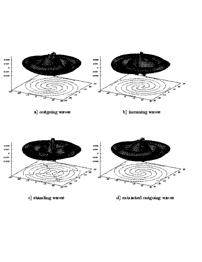
Figure 3: The $\Psi$ field for two rotating point sources in the equatorial plane. The fields shown are nonlinear solutions of Eqs. (4), (5) and (30), with $a\Omega=0.3$ and $\lambda=-1$. For clarity, the $\varphi$-average is removed at each radius. Parts (a) and (b) of the figure show, respectively, the nonlinear outgoing and ingoing solutions. Part (c) is the standing-wave solution, and part (d) is the outgoing solution extracted from it. The vertical scale gives field strength (arbitrary units) and the horizontal coordinates are corotating Cartesian coordinates in units of $a$, the distance of a source from the rotation axis.

Numerical results

We first illustrate the fundamental concept of the PSW method with various solutions of Eq. (5), with the nonlinearity given in Eq. (30) . Figure 3 shows solutions in the equatorial ($\theta=\pi/2$) plane; the amplitude of the field $\Psi$ is plotted as a function of corotating Cartesian coordinates $x=r\cos\varphi$, and $y=r\sin\varphi$. The source points are on the $x$ axis at $x=\pm a$, and the outer boundary is at $r=30a$. For all four plots, $a\Omega=0.3$, $\lambda=-1$ and $\Psi_{0}=0.15$. The results plotted are those from direct iteration with the FFT method, for a computational grid using 361 radial divisions, 16 divisions in $\theta$, and 32 Fourier modes. For all models, the computed results are dominated by the monopole, so for clarity in the figures the $\varphi$-average of the solution has been subtracted at every radius. It is worth noting that this procedure not only removes the monopole (the $\ell=0$ part of the solution), but also removes the $m=0$ part of the quadrupole, etc.

The plot in part (a) of Fig. 3 shows the outgoing solution (solution for outgoing boundary conditions); the plot in part (b) shows the corresponding ingoing solution. The plot in part (c) is the computed standing-wave solution for the same problem parameters. (Note: this nonlinear standing-wave solution is not half the superposition of the outgoing and ingoing solutions. Rather, it is the nonlinear field equation solved with the standing-wave definition discussed in Sec. II.) Part (d) shows the key idea of the PSW approximation, the outgoing solution extracted from the standing-wave solution, by the extraction method described in Eqs. (19)–(26). When the PSW method is used in general relativity, it will be possible only to compute the standing-wave solution; the extracted outgoing solution will represent the approximation to the physical, outgoing solution.

Table 1 gives quantitative results for strongly nonlinear outgoing waves. In that table, values are given for the reduction factor due to the nonlinearity. As explained following Eq. (31), this is the factor by which the nonlinearity decreases the amplitude of the waves. (For the same $a\Omega$ and source strength, the amplitude of outgoing waves for the linear problem $\lambda=0$ problem is compared to the amplitude for a problem with $\lambda\neq 0$.) The fact that the reduction factors are significantly different from 100% shows that we are able to compute models in which nonlinear effects are strong. In the table the computed reduction is compared with estimates from heuristic models of Eqs. (31)–(33) in which $\Psi$ is taken to have a Yukawa form very near the source, and a Coulomb form further out, but well within the near zone. The agreement of the computations with the estimates is strong evidence that the heuristic model captures much of the nature of the nonlinear effect.

Table 1: The reduction factor for outgoing waves due to the nonlinearity. For all cases, $\Psi_{0}=0.15$. The second column refers to Eq. (32). This equation is solved for $R_{\rm lin}$. Estimate 1 uses this value of $R_{\rm lin}$ in $\exp{(-\sqrt{-\lambda}R_{\rm lin})}$. Estimate 2 is the reduction factor found from a numerical solution of Eq. (33). The last column gives the results from Newton-Raphson computation with $a\Omega=0.3$, with the outer boundary at $r=30a$, and with a $r,\theta,\varphi$ grid of $120\times 20\times 32$.

$\lambda$	Estimate 1	Estimate 2	Computation
-1	69%	87%	78%
-2	62%	73%	68%
-5	53%	65%	55%
-10	46%	54%	47%
-25	37%	41%	35%

Table 2 gives information on the numerical errors of the most computationally intensive solution type: that for strongly nonlinear waves computed via Newton-Raphson iteration. A single physical model ($\lambda=-10$, $\Psi_{0}=0.15$, $a\Omega=0.3$, outer boundary at $r=30a$) is computed on five different grids. As a measure of the truncation error for grid $k$, the L2 difference (the square root of the average square difference) is found between the results for grid $k$ and for grid $k+1$ . This is listed in Table 2 as the error in grid $k$. These results, especially for the finest three grids, suggest quadratic convergence of the numerical process.

Table 2: Convergence of finite difference computations. Nonlinear outgoing solutions are computed with five different grid resolutions for $\lambda=-10$, $\Psi_{0}=0.15$, $a\Omega=0.3$ and outer boundary at $r=30a$. An $L2$ norm is computed for the difference between the solution for grid $k$ and grid $k+1$. This is reported as the “Error” for grid $k$.

$k$	$n_{r}\times n_{r}\times n_{\varphi}$	Error
1	90$\times$10$\times$16	2.71 E-5
2	120$\times$14$\times$22	1.60 E–5
3	150$\times$16$\times$26	8.68 E-6
4	180$\times$20$\times$32	5.22 E-6
5	210$\times$24$\times$38

The crux of the PSW method is that a good approximation to a nonlinear outgoing solution can be extracted from a standing wave nonlinear solution. Examples of this are given in the next two figures, the central numerical results in this paper.

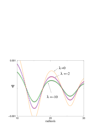
Figure 4: Extracted outgoing nonlinear waves vs. true outgoing nonlinear waves. For $\lambda=0,-2,-10$, $\Psi_{0}=0.15$, $a\Omega=0.3$, with a $180\times 20\times 32$ grid. The field $\Psi$ is shown as a function of r along a radial line through the source point, i.e. , along the $\theta=\pi/2$, $\varphi=0$ line. Continuous curves show computational results for outgoing waves. Discrete points, for the nonlinear models, show the approximate outgoing waves extracted from standing wave solutions.

Figure 4 shows results for computations of linear ($\lambda=0$) and nonlinear ($\lambda=-2$ and -10) models for $\Psi$ along the $\theta=\pi/2$, $\varphi=0$ lines. All models used rotation rate $a\Omega=0.3$ and nonlinearity parameter $\Psi_{0}=0.15$ and the $180\times 20\times 32$ grid with an outer boundary at $r=30a$. The nonlinear models were solved through Newton-Raphson iteration with continuation in $\lambda$. The figure shows, as continuous lines, the computed solutions for outgoing waves with $\lambda=0,-2,\,-10$. Included in the figure also are the $\lambda=-2,\,-10$ results for the approximate outgoing waves extracted from the nonlinear standing wave solutions by the method of Eq. (23). The difference between these outgoing approximations and the true outgoing waves is so small that the approximation results are given as discrete data points to aid in visualization.

Figure 5 shows the small-radius portions of the same models as those in Fig. 4. (The $\lambda=0$ curve is nearly indistinguishable from that for $\lambda=-2$, and is omitted from the figure.) The radial $\theta=\pi/2$, $\varphi=0$ line along which the results are presented, goes through the source point at $r=a$, so Fig. 5 shows the computed solution in the neighborhood of the source. The Yukawa-like effect of the nonlinearity near the source is evident in more rapid fall-off of the $\lambda=-10$ model away from the source point.

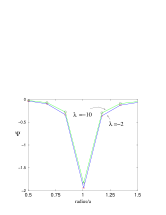
Figure 5: The same models as in Fig. 4, but in the region of the sources. As in Fig. 4 continuous curves show the computations of the true nonlinear outgoing waves, and discrete points show the outgoing wave approximation extracted from the nonlinear standing wave solution.

The results in Figs. 5 and 4 are graphical evidence for the accuracy of the PSW method; the outgoing waveforms extracted from the nonlinear standing wave solution are excellent approximations to the true outgoing waves both near the sources and in the wave zone. The agreement in the intermediate zone (not shown in the figures) is equally impressive. A quantitative measure of the agreement is the “L2” difference of the outgoing wave and the extracted outgoing approximation. This measure is the square root of the average (over all grid points) of the squared difference between the true and the extracted outgoing solutions. For $\lambda=-10$ this L2 difference is $8.7\times 10^{-6}$ and is of the same order as the error in Table 2 for the $180\times 20\times 32$ grid being used. Since the numerical uncertainties are of the same order as the difference between the true and the extracted outgoing waves we cannot claim to have computed any meaningful inaccuracy in the PSW approximation.

This is unfortunate. In presenting numerical results it would be useful to demonstrate that the PSW approximation is, after all, an approximation by showing a model in which the extracted outgoing solution is significantly different from the true outgoing solution. Our inability to do this is related to limitations on numerical solutions. Our arguments for effective linearity show that the PSW approximation should fail only if the region of significant nonlinearity overlaps the wave zone. For this reason we used the $\chi$-dependent prefactor of Eq. (36) in an earlier version of the present paper to allow us to force the nonlinearity to be concentrated in the wave zone. Although that technique did allow us to induce significant errors in the PSW approximation, we have explained, following Eq. (36), why the solutions for the models with the prefactor have undesirable features. If no unnatural $\chi$-dependence is explicitly injected in the source, the way in which effective nonlinearity can be made to fail is for $a\Omega$ to approach unity, i.e. , for the source points to move very relativistically (a case in which the PSW would be expected to fail for binary inspiral). Unfortunately, we have not been able to find convergent solutions for large $a\Omega$. Presumably this is due to the fact that large $a\Omega$ means fields with sharp gradients, too sharp to be handled by our necessarily coarse grids.

IV Conclusions

We have given here the foundations of the PSW method based on the extraction of an outgoing solution from a computed standing-wave solution. We have also given the details of the extraction calculation.

The results provided for convergent nonlinear models are “proof” by example that there is no fundamental mathematical problem of well-posedness of the mixed PDE problem, with radiative boundary conditions on a sphere that is in both the elliptic and hyperbolic regions of the problem. We have, furthermore, presented limited numerical evidence for the validity of the PSW method, i.e. , that the extracted outgoing solution is a good approximation to the true nonlinear outgoing solution. This evidence helps make the case for the application of the method to the general relativistic problem, in which only the standing-wave solution will be computable, and the extracted solution will be taken as the approximation to the physical problem.

The numerical studies have also taught a lesson about the limitations of the relatively straightforward numerical method used here, matrix inversion of the finite difference equations in spherical coordinates. We have found that this method is limited by the coarse grid that can be used for the finite-differencing. We could, in principle, use a software engineering approach to increase the range of nonlinearity and rotation rate that can be handled. But the methods used here, spherical coordinates and delta function sources, are meant only to provide a relatively simple context for establishing the foundations for more advanced approaches.

In a paper now in preparationpaperII , we will present an important step forward in dealing with PSW problems, a coordinate system that conforms to the geometry near the sources and far from the source asymptotically goes to spherical polar coordinates, the coordinates best suited to the description of the waves. One advantage of this method is that it allows us very simply to put in details of the sources as inner boundary conditions rather than point sources. In addition, the new coordinates turn out to be very well suited to a spectral method that has shown remarkable computational efficiency, but that poses new computational problems. Computations using an adapted coordinate system have already been carried out for the three-dimensional nonlinear scalar problem with both the finite difference and spectral formulation, and for linearized general relativity using the finite difference formulation. Since the details of adapted coordinates, especially with the unusual spectral method, are not directly related to the foundations of the PSW method, those details are appropriate to a separate paper.

A very different approach to better numerics is to use relaxation methods, already mentioned in Sec. III. In view of the large number of uncertainties about their application, we have started on a basic study of relaxation methods in mixed PDE systems in PSW-type problems, but will continue to explore a number of different numerical approaches to the PSW problem.

V Acknowledgment

We gratefully acknowledge the support of the National Science Foundation under grants PHY9734871 and PHY0244605. We also thank the University of Utah Research Foundation for support during this work. We thank Christopher Johnson and the Scientific Computing and Imaging Institute of the University of Utah for time on their supercomputers to produce the non-FFT results of Sec. III. We have also made use of supercomputing facilities provided by funding from JPL Institutional Computing and Information Services and the NASA Offices of Earth Science, Aeronautics, and Space Science. We thank John Friedman and Kip Thorne for helpful discussions and suggestions about this work.

References

- (1) G. Gonzalez, gravitational wave detectors: A report from LIGO-land, in Recent Developments in Gravity: Proceedings of the 10th Hellenic Relativity Conference, K. D. Kokkotas and N. Stergioulas (Eds.), (World Scientific, Singapore, 2003); [gr-qc/0303117]
- (2) F. Acernese et al., Class. Quant. Grav. 20, 609 (2003).
- (3) H. Lück et al., in Gravitational Waves, Third Edoardo Amaldi Conference held in Pasadena, CA 12-16 July, 1999, S. Meshkov (Ed), AIP Conference Proceedings, Vol. 523 (AIP Press, New York, 2000), pp. 119–127.
- (4) M. Ando, Current status of the TAMA300 interferometer, prepared for 2nd Workshop on Gravitational Wave Detection, Tokyo, Japan, 19-22 Oct 1999.
- (5) E. Colbert and A. Ptak, Astrophys. J. Supp. 143, 25 (2002).
- (6) B. F. Schutz, in Lighthouses of the Universe – The Most Luminous Celestial Objects and Their Use for Cosmology: Proceedings of the Mpa/Eso/Mpe/Usm Joint Astronomy Conference, C. K. Chui, R. A. Siuniaev, and E. Churazov (Eds.) (Springer-Verlag, New York, 2002), pp. 207–224; [gr-qc/0111095].
-
(7)
See
http://lisa.jpl.nasa.gov. - (8) M. A. Scheel et al., Phys. Rev. D66, 124005 (2002).
- (9) H.-J. Yo, T. W. Baumgarte, and S. L. Shapiro, Phys. Rev. D66, 084026 (2002).
- (10) J. Baker et al., Phys. Rev. D 65, 124012 (2002).
- (11) J. K. Blackburn and S. Detweiler, Phys. Rev. D 46, 2318 (1992).
- (12) S. Detweiler, Phys. Rev. D 50, 4929 (1994).
- (13) J. Friedman, private communication.
- (14) C. W. Misner, K. S. Thorne and J. A. Wheeler, Gravitation (Freeman, San Francisco, 1973), Sec. 20.3.
- (15) J. T. Whelan, W. Krivan, and R. H. Price, Class. Quant. Grav. 17, 4895 (2000).
- (16) R. H. Price, Class. Quant. Grav. 21, S281-S293 (2004).
- (17) A. Ashtekar et al., Phys. Rev. Lett. 85, 3564 (2000).
- (18) J. W. York, Jr., Phys. Rev. Lett. 26, 1656 (1971).
- (19) J. W. York, Jr., J. Math. Phys. 14, 456 (1973).
- (20) Z. Andrade et al., paper in preparation.
- (21) G. W. Gibbons and J. M. Stewart, in Classical General Relativity, edited by W. B. Bonnor, J. N. Islam, and M. A. H. MacCallum (Cambridge University Press, Cambridge, 1983), pp. 77—94.
- (22) J. L. Friedman, K. Uryu, and M. Shibata, Phys. Rev. D 65, 064035 (2002).
- (23) For the problem in Eq. (5) has been shown to be well posed for a range of source functions and boundary conditions; C. Torre, math-ph/0309008.
- (24) C. Ferrari and F. G. Tricomi, Transonic Aerodynamics (Academic Press, New York, 1968); J. D. Cole and L. P. Cook, Transonic Aerodynamics (North-Holland, Amsterdam, 1986).
- (25) This is an expanded version of an argument given in the two-dimensional context in Ref. WKP .
- (26) J. T. Whelan, C. Beetle, W. Landry, and R. H. Price, Class. Quant. Grav. 19, 1285 (2002).
- (27) This form was used in early versions of the present paper, is described in Ref. safari , and is closely related to the nonlinearity used in Ref. WKP .
- (28) E. M. Murman and J. D. Cole, AIAA J. 9, 114 (1971).
- (29) D. Nixon, in Computational methods and problems in aeronautical fluid dynamics, edited by B. L. Hewit (Academic Press, New York, 1976), pp. 290–326.