Maintaining Information in Fully-Dynamic Trees with Top Trees

Abstract

We introduce top trees as a design of a new simpler interface for data structures maintaining information in a fully-dynamic forest. We demonstrate how easy and versatile they are to use on a host of different applications. For example, we show how to maintain the diameter, center, and median of each tree in the forest. The forest can be updated by insertion and deletion of edges and by changes to vertex and edge weights. Each update is supported in $O(\log n)$ time, where $n$ is the size of the tree(s) involved in the update. Also, we show how to support nearest common ancestor queries and level ancestor queries with respect to arbitrary roots in $O(\log n)$ time. Finally, with marked and unmarked vertices, we show how to compute distances to a nearest marked vertex. The later has applications to approximate nearest marked vertex in general graphs, and thereby to static optimization problems over shortest path metrics.

Technically speaking, top trees are easily implemented either with Frederickson’s topology trees [Ambivalent Data Structures for Dynamic 2-Edge-Connectivity and $k$ Smallest Spanning Trees, SIAM J. Comput. 26 (2) pp. 484–538, 1997] or with Sleator and Tarjan’s dynamic trees [A Data Structure for Dynamic Trees. J. Comput. Syst. Sc. 26 (3) pp. 362–391, 1983]. However, we claim that the interface is simpler for many applications, and indeed our new bounds are quadratic improvements over previous bounds where they exist.

1 Introduction

In this paper, we introduce top trees as a new simpler interface for data structures maintaining information in a fully-dynamic forest. Here fully-dynamic means that edges may be both inserted and deleted. The information could be, say, the diameter of each tree in the forest. However, if the tree is a minimum spanning tree of a dynamic graph, the information could help changing the minimum spanning tree as the graph changes.

Technically speaking, top trees are easily implemented either with Frederickson’s topology trees [14] or with Sleator and Tarjan’s dynamic trees [30]. The contribution of top trees is the design of an interface providing users with easier access to the full power of these advanced techniques.

Targeting a broad audience of potential users, the bulk of this paper is like a tutorial where we demonstrate the flexibility of top trees in different types of applications:

• We re-derive some of the classic applications from [14, 30], e.g., finding the maximum weight of a given path.

• We improve some previous bounds. More specifically, we show how to maintain the centers and medians of trees in a dynamic forest in $O(\log n)$ time per updates. The previous bounds were $O(\log^{2}n)$ time [7, 3].

• We consider problems that appear not to have been studied before for a dynamic forest. For example, we show how to maintain the diameters of trees in a dynamic forest. We also show how to answer level ancestor and nearest common ancestor queries with respect to arbitrary roots. Finally, with marked and unmarked vertices, we show how to compute distances to a nearest marked vertex. In all of these cases, we support both updates and queries in logarithmic time. The marking result has applications to approximate nearest marked vertex in general graphs, and thereby to static optimization problems over shortest path metrics.

We note that finding medians and centers is more difficult than, e.g., finding the minimum edge on a given path because they are “non-local” properties. Here, by a local property we mean that if an edge or a vertex has the property in a tree, then it has the property in all subtrees it appears in. Local properties lend themselves nicely to bottom-up computations, whereas non-local properties tend to be more challenging. Building on top of our top trees, we present here a quite general technique for dealing with non-local properties.

We implement our top trees with Frederickson’s topology trees [14], which we in turn implement with Sleator and Tarjan’s st-trees [30]. The implementation of topology trees with st-trees was not known. It has the interesting consequence that the simple amortized version of st-trees gives a simple amortized version of topology trees.

We note that since top trees were originally announced [1], they have found applications in other works [16, 22, 33]. All these applications rely on results presented in this paper. Also, our specific result for dynamic tree diameters has found its own application in [25].

1.1 Preliminaries

Most of this paper concerns a forest of trees, which means that if vertices $v$ and $w$ are connected, they are connected by a unique path, which we shall denote $v\cdots w$.

When we talk about an edge $(v,w)$, on an implementation level, we often really think of an identifier $e$ of the undirected edge with end-points $v$ and $w$. Via arrays, the end-points can be found from the identifier $e$ in constant time. However, other information can also be associated with $e$ such as its successor and predecessor in the incidence lists around $v$ and $w$.

1.2 Contents

The paper is organized as follows. In § 2 we introduce top trees and solve the diameter problem. In § 3 we present our technique for non-local problems, and solve the center and median problems. In § 4 we discuss the advantages and limitations of using top trees relative to other data structures for dynamic trees. In § 5 we mention some generalizations of top trees used in later papers. Finally, in § 6 we implement top trees with topology trees and topology trees with st-trees. Finally, we have some concluding remarks in § 7.

2 Top Trees

A top tree is defined based on a pair consisting of a tree $T$ and a set $\partial{T}$ of at most 2 vertices from $T$, called external boundary vertices. Given $(T,\partial{T})$, any subtree $C$ of $T$ has a set $\partial_{(T,\partial{T})}C$ of boundary vertices which are the vertices of $C$ that are either in $\partial{T}$ or incident to an edge in $T$ leaving $C$. Here, by a subtree of an undirected tree, we mean any connected subgraph. The subtree $C$ is called a cluster of $(T,\partial{T})$ if it has at least one edge and at most two boundary vertices. Then $T$ is itself a cluster with $\partial_{(T,\partial{T})}T=\partial{T}$. Also, if $A$ is a subtree of $C$, $\partial_{(C,\partial_{(T,\partial{T})}C)}A=\partial_{(T,\partial{T})}A$, so $A$ is a cluster of $(C,\partial_{(T,\partial{T})}C)$ if and only if $A$ is a cluster of $(T,\partial{T})$. Since $\partial_{(T,\partial{T})}$ is a canonical generalization of $\partial$ from $T$ to all subtrees of $T$, we will use $\partial$ as a shorthand for $\partial_{(T,\partial{T})}$ in the rest of the paper.

A top tree $\mathcal{R}$ over $(T,\partial{T})$ is a binary tree such that:

1. The nodes of $\mathcal{R}$ are clusters of $(T,\partial{T})$.

2. The leaves of $\mathcal{R}$ are the edges of $T$.

3. Sibling clusters are neighbors in the sense that they intersect in a single vertex, and then their parent cluster is their union (see Fig. 1).

4. The root of $\mathcal{R}$ is $T$ itself.

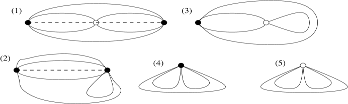
Figure 1: The cases of joining two neighboring clusters into one. The $\bullet$ are the boundary vertices of the joined cluster and the $\circ$ are the boundary vertices of the children clusters that did not become boundary vertices of the joined cluster. Finally the dashed line is the cluster path of the joined cluster.

A tree with a single vertex has an empty top tree. The basic philosophy is that clusters are induced by their edges, the vertices only being included as their end-points. This is why clusters need at least one edge, and we note that neighboring clusters are induced by disjoint edge sets inducing a common vertex.

We will sometimes refer to the tree $T$ as the underlying tree to differentiate it from the top tree $\mathcal{R}$.

The top trees over the trees in our underlying forest are maintained under the following forest updates:

• where $v$ and $w$ are in different trees, links these trees by adding the edge $(v,w)$ to our dynamic forest.

• removes the edge $e$ from our dynamic forest.

• where $v$ and $w$ are in the same tree $T$, makes $v$ and $w$ the external boundary vertices of $T$. Moreover, expose returns the new root cluster of the top tree over $T$.

  expose can also be called with zero or one vertices as argument if we want less than two external boundary vertices. If expose is called with zero arguments, as $\textnormal{{expose}}()$, it does not return a root cluster. This is because there may be multiple trees, and without an argument, expose cannot know what tree we are interested in. Finally, it is guaranteed that $\textnormal{{expose}}()$ does not change the structure of the top trees. It only affects some of the boundaries of the clusters in the top trees.

In general, link and cut make the set of external boundary vertices for the resulting trees empty. To accommodate these forest updates, the top trees are changed by a sequence of local top tree modifications described below. During these modifications, we will temporarily accept a partial top tree whose root cluster may not be a whole underlying tree $T$ but just a cluster of $T$.

• creates a top tree with a single cluster $e$ which is just an edge.

• where $A$ and $B$ are neighboring root clusters of two top trees $\mathcal{R}_{A}$ and $\mathcal{R}_{B}$. Creates a new cluster $C=A\cup B$ and makes it the common root of $A$ and $B$, thus turning $\mathcal{R}_{A}$ and $\mathcal{R}_{B}$ into a single new top tree $\mathcal{R}_{C}$. Finally, the new root cluster $C$ is returned.

• where $C$ is the root cluster of a top tree $\mathcal{R}_{C}$ and has children $A$ and $B$. Deletes $C$, thus turning $\mathcal{R}_{C}$ into the two top trees $\mathcal{R}_{A}$ and $\mathcal{R}_{B}$. Finally, the root clusters of $\mathcal{R}_{A}$ and $\mathcal{R}_{B}$ are returned.

• eliminates the top tree consisting of edge $e$.

2.1 Discipline for modifying top trees

Top tree modifications have to be applied in the following order:

1. First, top-down, we perform a sequence of splits.

2. Then we destroy the clusters of some edges.

3. Then we update the forest.

4. Then we creates clusters of some edges.

5. Finally, with joins, we recreate the top tree bottom-up.

The above order implies that when we do a split or join, we know that all parts of the underlying forest is partitioned into base clusters.

It is an important rule that a forest update may not change any current cluster. Here, a cluster is changed by a forest update if the update changes its set of edges or its set of boundary vertices. To appreciate the latter, consider an update $\textnormal{{expose}}(v)$. This update only changes clusters with $v$ an interior vertex. A cluster in which $v$ is already a boundary vertex is not changed. Satisfying the rule means that when we get to the update in step 3, the previous steps 1–2 should have eliminated all clusters that would be changed by the update.

It is often natural to perform a composite sequence of updates in step 3. For example, if dealing with a spanning tree $T$, we might want to swap one tree edge $(v_{1},w_{1})$ with another edge $(v_{2},w_{2})$. If we do $\left\langle\textnormal{{cut}}((v_{1},w_{1}));\textnormal{{link}}((v_{2},w_{2})\right\rangle$ as a composite update rather than as two separate updates, we avoid dealing with a temporary forest when we do the top tree modifications in steps 1–2 and 4–5.

In this paper, we are going to show the following result:

Theorem 1

For a dynamic forest we can maintain top trees of height $O(\log n)$ supporting each link, cut, or expose with a sequence of $O(1)$ create and destroy, and $O(\log n)$ join and split. These top tree modifications are identified in $O(\log n)$ time. The space usage of the top trees is linear in the size of the dynamic forest. For a composite sequence of $k$ updates, each of the above bounds are multiplied by $k$.

The proof of Theorem 1 is deferred to § 6. Until then, the focus will be on applications of top trees.

2.2 Top trees generalize balanced binary search trees

Put in perspective, our top trees are natural generalizations of standard balanced binary trees over dynamic collections of lists that may be concatenated and split. In the balanced binary trees, each node represents a segment of a list, which in top terminology is just a special case of a cluster. Standard implementations for balanced binary trees also ascertain that the height is $O(\log n)$, and that each concatenation and split can be done by $O(\log n)$ local modifications.

2.3 Top tree terminology

If a vertex in a cluster is not a boundary vertex, it is internal to that cluster. If a cluster $C$ has two boundary vertices $a$ and $b$, we call $C$ a path cluster and $a\cdots b$ the cluster path of $C$, denoted $\pi(C)$. If $C$ has only one boundary vertex $a$, $C$ is called a point cluster and then $\pi(C)=a$. Note that if $A$ is a child cluster of $C$ and $A$ shares an edge with $\pi(C)$, then $\pi(A)\subseteq\pi(C)$, and then we call $A$ a path child of $C$. In terms of boundary vertices, if $C$ has children $A$ and $B$, $A$ is a path child of $C$ if and only if $\left\lvert{\partial{C}}\right\rvert=2$ and either $\partial{A}=\partial{C}$ (Fig. 1 (2)) or $\partial{C}\subset\partial{A}\cup\partial{B}$ (Fig. 1 (1)).

2.4 Representation and usage of top trees

A top tree is represented as a standard binary rooted tree with parent and children pointers. The nodes used to represent the top tree are denoted top nodes. The top nodes of the binary tree represent the clusters, and with each top node is associated the set of at most two boundary vertices of the represented cluster. With a top leaf we store the corresponding edge. With an internal top node is stored how it is decomposed into its children (c.f. Fig. 1). Thus, considering the information descending from a top node, we can construct the cluster it represents. Finally, from each vertex $v$, there is a pointer to the smallest cluster $C(v)$ that $v$ is internal to, or to the root cluster containing $v$ if $v$ is an external boundary vertex.

Following parent pointers from $C(v)$, we can find the root, $top\_root(v)$, of the top tree over the underlying tree $T$ containing $v$. In the case of a forest, two vertices $v$ and $w$ are in the same underlying tree if and only if $top\_root(v)=top\_root(w)$. With top trees of logarithmic height as in Theorem 1, we identify $top\_root(v)$ in $O(\log n)$ time.

An application of the top tree data structure, such as maintaining diameters, centers, or medians, has direct access to the above representation, and will typically associate some extra information with the top nodes. The application employs an implementation of top trees, which is an algorithm like the one described in Theorem 1, converting each link, cut, or expose into a sequence of splits and joins on the top trees. In connection with each join and split the application is notified and given pointers to the top nodes representing the involved clusters. The application can then update its information associated with these top nodes. We note that a top tree may only be modified with split and join. This discipline is important if we have several applications running over the same top trees, each maintaining its own information as splits and joins are performed. Typically, link and cut are operations imposed from the outside whereas expose typically is used internally by an application.

2.5 Concrete applications

As a first example, we can now easily derive a main result from [30].

Theorem 2 (Sleator and Tarjan)

We can maintain a dynamic collection of weighted trees in $O(\log n)$ time per link and cut, supporting queries about the maximum weight between any two vertices in $O(\log n)$ time.

Proof:

For this application, with each (top node representing a) cluster $C$, we store as extra information the maximum weight $max\_weight(C)$ on the cluster path $\pi(C)$. For a point-cluster $C$, $max\_weight(C)=-\infty$. If a path cluster consists of a single edge $e$, $max\_weight(e)$ is just the weight of the edge. When a path cluster $C$ is created by a join, $max\_weight(C)$ is the maximum weight stored at its path children. When $C$ is split or destroyed, we just discard the information stored with $C$. Now, to find the maximum weight between $v$ and $w$, we set $C:=$ $\textnormal{{expose}}(v,w)$. Then $\pi(C)=v\cdots w$, and we return $max\_weight(C)$. Since join and split are supported in constant time, the Theorem now follows from Theorem 1.  

In the above example, split is trivial. To see the relevance of split, we consider an extension from [30].

Theorem 3 (Sleator and Tarjan)

In Theorem 2, we can also add a common weight $x$ to all edges on a given path $v\cdots w$ in $O(\log n)$ time.

Proof:

For this extension, for each cluster $C$, we introduce a “lazy” weight $extra(C)$ which is to be added to all edges in $\pi(C)$ in all clusters properly descending from $C$. We note that if $C$ is a root cluster, $max\_weight(C)$ is not affected by these $extra$-values, so $max\_weight(C)$ is the correct maximal weight on $\pi(C)$. In particular, we can still find the maximal weight between $v$ and $w$ as $max\_weight(\textnormal{{expose}}(v,w))$.

The addition of $x$ to $v\cdots w$ is now done by calling $C:=\textnormal{{expose}}(v,w)$ and adding $x$ to $max\_weight(C)$ and to $extra(C)$. Then $\textnormal{{split}}(C)$ requires that for each path child $A$ of $C$, we set $max\_weight(A):=max\_weight(A)+extra(C)$ and $extra(A):=extra(A)+extra(C)$. For $C:=\textnormal{{join}}(A,B)$, we set $max\_weight(C):=\max\left\{{max\_weight(A),max\_weight(B)}\right\}$ and $extra(C):=0$. Finally, to find the maximum weight on the path $v\cdots w$, we set $C:=\textnormal{{expose}}(v,w)$ and return $max\_weight(C)$.  

We will now go beyond [30] with a further extension needed in [33].

Theorem 4

In Theorem 3, we can also ask for the maximum weight of the underlying tree containing a vertex $v$ in $O(\log n)$ time.

Proof:

Elaborating on the information from the previous two proofs, for each cluster $C$, we will maintain a variable $max\_non\_path(C)$ denoting the maximal weight on an edge in $C$ which is not on the cluster path. Assuming this variable, we can find the maximal weight of the underlying tree containing $v$, setting $C:=top\_root(v)$ and returning $\max\{max\_non\_path(C),max\_weight(C)\}$.

We maintain the $max\_non\_path$ variables as follows. When the cluster of an edge $e$ is created, if $e$ has two boundary vertices, we set $max\_non\_path(e)=-\infty$. Otherwise, $max\_non\_path(e)$ is set to the weight of $e$. When a cluster is joined as $C:=\textnormal{{join}}(A,B)$, we first set $max\_non\_path(C):=\max\{max\_non\_path(A),max\_non\_path(B)\}$. If $C$ is not a path cluster but one of its children, say $A$, is a path cluster (c.f. Fig. 1(3)), then we further have consider weights from the cluster path of $A$, setting $max\_non\_path(C):=\max\{max\_non\_path(C),max\_weight(A)\}$. We note here that because $A$ was a root cluster, $max\_weight(A)$ has its correct value, not missing any $extra$-values from at ascending clusters. When clusters are split or destroyed, this has no impact on the $\max\_non\_path$-variables.  

In the rest of this paper, we are more interested in distances than in maximum weights. Modifying the proof of Theorem 2, for each cluster $C$, we will maintain the length $length(C)$ of the cluster path. The length is maintained as the maximum weight except that if $C$ is created by a join, $length(C)$ is the sum of lengths stored with its path children. Thus we have

Lemma 5

In top trees, for each cluster $C$, we can maintain the length, denoted $length(C)$, of the cluster path in constant time per local top update, hence in $O(\log n)$ time per link or cut. Then the distance between two vertices $v$ and $w$ can be found in $O(\log n)$ time as $length(\textnormal{{expose}}(v,w))$.  

As an interesting new application of top trees, we get the claimed result for dynamic diameters.

Theorem 6

We can maintain a dynamic collection of weighted trees in $O(\log n)$ time per link and cut, supporting queries about the diameter of the tree containing any vertex in $O(\log n)$ time.

Proof:

For each cluster $C$, we store its diameter $diam(C)$. Moreover, for each of its boundary vertices $a\in\partial{C}$, we store the maximal distance $max\_dist(C,a)$ from $a$ to any vertex in $C$. Finally, we maintain the cluster length from Lemma 5. The variables $max\_dist$ and $length$ are auxiliary fields, needed for a fast join. Such carefully chosen extra information is often crucial in top tree applications.

When the cluster of an edge $e$ is created, $diam(e)=weight(e)$, and for each boundary vertex $v$ of $e$, $max\_dist(e,v)=weight(e)$. Now, suppose $C:=\textnormal{{join}}(A,B)$, and that $c$ is the common boundary vertex of $A$ and $B$. Then we set

$$diam(C):=\max\left\{{diam(A),diam(B),max\_dist(A,c)+max\_dist(B,c)}\right\}$$

Now consider any boundary vertex $a$ of $C$. By symmetry, we may assume that if $a$ is not in one of $A$ and $B$, it is not in $B$. Let $c$ be the intersection vertex of $A$ and $B$. Then, if $c\neq a$,

$$max\_dist(C,a)=\max\left\{{max\_dist(A,a),length(A)+max\_dist(B,c)}\right\}$$

If $c=a$ then

$$max\_dist(C,c)=\max\left\{{max\_dist(A,c),max\_dist(B,c)}\right\}$$

Thus, create and join are implemented in constant time. As in the proof of Theorem 2, split and destroy do not require any action. Hence Theorem 1 implies that we can maintain the above information in $O(\log n)$ time per link or cut. To answer a diameter query for a vertex $v$, we set $C:=\textnormal{{expose}}(v)$ and return $diam(C)$.  

Another illustrative application is the maintenance of nearest marked neighbors.

Theorem 7

We can maintain a dynamic collection of trees in $O(\log n)$ time per link and cut, or marking and unmarking of a vertex, supporting queries about the (distance to) the nearest marked vertex of any given vertex in $O(\log n)$ time.

Proof:

Below, we just focus on finding the distance to the nearest marked vertex. This is easily extended to also providing the vertex.

For each boundary vertex $a$ of a cluster $C$, we maintain the distance $mark\_dist(C,a)$ from $a$ to the nearest marked vertex in $C\setminus\partial{C}$. The reason that why exclude the boundary of $C$ from consideration is that a vertex $v$ may appear as boundary vertex of $\Omega(n)$ clusters, and all these would be affected, if $v$ was (un)marked. From $mark\_dist(C,a)$ we can easily compute the distance $mark\_dist^{*}(C,a)$ from $a$ to the nearest marked vertex in $C$ excluding only boundary vertices different from $a$. Then $mark\_dist^{*}(C,a)=0$ if $a$ is marked, and $mark\_dist^{*}(C,a)=mark\_dist(C,a)$ if $a$ is unmarked. We also maintain the cluster path length, $length(C)$, as in Lemma 5.

Given a vertex $u$, to find the distance to the nearest marked vertex, we simply set $C:=\textnormal{{expose}}(u)$, and return $mark\_dist^{*}(C,u)$.

To (un)mark a vertex $v$, we first expose $v$. As an external boundary vertex, $v$ has no impact on any $mark\_dist$-value, so we can freely (un)mark it.

Suppose the cluster $C$ is created as an edge $(v,w)$. Then $mark\_dist(C,v)$ is the weight of $(v,w)$ if $w$ is marked and not in the boundary; otherwise, we it to infinity.

Finally, consider $C:=\textnormal{{join}}(A,B)$ with $\{c\}=A\cap B$. Let $a$ be a boundary vertex of $C$. By symmetry, we can assume that $a$ is in $A$. We now have $mark\_dist(C,a)=$

$$\left\{\begin{array}[]{ll}\min\{mark\_dist(A,a),mark\_distB,a)\}&\mbox{if $a=c$}\\ \min\{mark\_dist(A,a),length(A)+mark\_dist(B,c)\}&\mbox{if $a\neq c$ and $c\in\partial{C}$}\\ \min\{mark\_dist(A,a),length(A)+mark\_dist^{*}(B,c)\}&\mbox{if $a\neq c$ and $c\not\in\partial{C}$}\end{array}\right.$$

Thus, we can support both join and create in constant time, and split and destroy do not require any action. By Theorem 1, this completes the proof of Theorem 7  

Corollary 8

For any positive integer parameter $k$, in a fixed undirected graph on $n$ vertices and $m$ edges, in $O(kmn^{1/k}\log n)$ expected time we can build an $O(kn^{1+1/k})$ space data structure, supporting (un)marking of vertices and queries about stretch $2k-1$ distances to a nearest marked vertex. Here stretch $2k-1$ means that the reported distance may be up to a factor $2k-1$ too long. Both queries and updates take $O(kn^{1/k}\log n)$ time.

Proof:

In [34], it is shown how to generate a cover of edge-induced trees within the above preprocessing bounds so that each vertex $v$ is in $O(kn^{1/k})$ trees, and if the distance from $v$ to $w$ is $d$, there is a tree in which the distance is at most $(2k-1)d$. Now, if a vertex is marked, it is marked in all the trees containing it, and to find a stretch $2k-1$ distance to a nearest marked vertex, we find the shortest distance to a marked vertex over all the trees.  

The above corollary is interesting because it in [18] is shown that several combinatorial optimization problems can be approximated efficiently on metrics with dynamic nearest neighbor. For example, in the bottle-neck matching problem, where we wish to minimize the furthest distance between a pair in the matching, we now get a $4k-2$ approximation in $\tilde{O}(mn^{1/k})$ expected time. An exact solution currently requires $\tilde{O}(mn+n^{2.5})$ time [12].

3 Non-Local searching

We are now going to build a black box on top of our top trees for maintenance of centers and medians. As discussed in the introduction, the common feature of centers and medians is that they represent non-local properties. Here a vertex/edge property is local if it being satisfied by a vertex/edge in a tree implies that the vertex/edge satisfies the property in all subtrees containing it. For example, being the minimum edge on a given path is a local property. Local properties lend themselves nicely to bottom-up computations whereas non-local properties appear to be more challenging.

For our general non-local searching, the application should supply a function select that given the root cluster of a top tree, selects one of the two children. Recall here that a root cluster represents the whole underlying tree, which is important when dealing with non-local properties. Our black box will use select to guide a binary search after a desired edge. More precisely, the first time select is called, it is just given the root of an original top tree $\mathcal{R}$. It then selects one of the two children. In subsequent iterations, there will be some cluster $C$ in the original top tree which is the intersection of all clusters selected so far. If $C$ has children $A$ and $B$, the black box modifies the top tree so that $A$ and $B$ are subsumed by different children $A^{*}$ and $B^{*}$ of the root. Then select is called on the root $C^{*}=\textnormal{{join}}(A^{*},B^{*})$. If $A^{*}$ is selected, $A$ is the new intersection of all selected clusters. Likewise, if $B^{*}$ is selected, $B$ is the new intersection of all selected clusters. This way, select is used to guide a binary search down through the original top tree $\mathcal{R}$. The formal statement of the result is as follows.

Theorem 9 (Non-Local Search)

Starting with the root cluster of a top tree of height $h$ and at most one external boundary vertex, after $O(h)$ calls to select, join, and split, there is a unique edge $(v,w)$ contained in all clusters chosen by select, and then $(v,w)$ is returned. Subsequently, the top tree is returned to its previous state with $O(h)$ calls to join, and split.

If there are two external boundary vertices $x$ and $y$, the above selection process will stop with a unique $(v,w)$ edge on the path from $x$ to $y$.

As stipulated in the general interface to top trees, the implementation behind Theorem 9 will only manipulate the top tree with join and split operations. In our applications, we will apply Theorem 9 to a top tree from Theorem 1 with height $h=O(\log n)$. Then the number of calls to join and split in Theorem 9 is $O(h)=O(\log n)$.

Theorem 9 will not be proved till § 3.4. Before that we demonstrate applications of Theorem 9 in the dynamic center, median, and ancestor problems. In these applications, our general approach is to first decide the information needed for select, second show how to make the information available. The external boundary vertices will only play a role in the ancestor application in §3.3.

3.1 Dynamic center

For any tree $T$ and vertex $v$ let $max\_dist(T,v)$ denote the maximal distance from $v$ in $T$. A center is a vertex $v$ minimizing $max\_dist(T,v)$.

Lemma 10

Let $T$ be a tree, and let $A$ and $B$ be neighboring clusters with $A\cap B=\left\{{c}\right\}$ and $A\cup B=T$. If $max\_dist(A,c)\geq max\_dist(B,c)$, $A$ contains all centers.

Proof:

Let $w$ be a vertex in $A$ of maximal distance to $c$. Then $dist(c,w)=max\_dist(A,c)=max\_dist(T,c)$. Now, for any $v\in B\setminus A$, $max\_dist(T,v)\geq dist(v,w)=dist(v,c)+dist(c,w)=dist(v,c)+max\_dist(T,c)$. Since the edge weights are positive, $dist(v,c)>0$, thus $max\_dist(T,v)>max\_dist(T,c)$ and $v$ cannot be a center.  

In the dynamic center problem, we maintain a forest under link and cut interspersed with queries $center(u)$ requesting the center of the current tree containing the vertex $u$. We use the top trees from Theorem 1. For each boundary vertex $a$ of a cluster $C$, we maintain the maximal distance $max\_dist(C,a)$ from $a$ in $C$ as described in the proof of Theorem 6. Then link and cut take $O(\log n)$ time.

To find $center(u)$, we first set $D:=\textnormal{{expose}}(u)$ so that $D$ becomes the current root cluster over the tree containing $u$. The non-local search of Theorem 9 will start in $D$, but we need to define select given an arbitrary root cluster $C$ with children $A$ and $B$, $A\cap B=\left\{{c}\right\}$. If $max\_dist(A,c)\geq max\_dist(B,c)$, select picks $A$, otherwise it picks $B$. By Lemma 10, any cluster picked contains all centers, so, following Theorem 9, the returned edge $(v,w)$ contains all centers. Moreover, select takes constant time, so $(v,w)$ is found in $O(\log n)$ time. To find out if $v$ or $w$ is a center, we compute $D:=\textnormal{{expose}}(v,w)$ in $O(\log n)$ time. Since $D$ coincides with $T$, we can return $v$ if $max\_dist(D,v)<max\_dist(D,w)$; $w$ otherwise. Hence we can answer $center(u)$ in $O(\log n)$ time. Thus we conclude

Theorem 11

The center can be maintained dynamically under link, cut and $center(u)$ queries in $O(\log n)$ worst case time per operation.

3.2 Dynamic median

Let $T$ be a tree with positive vertex and edge weights. A median is a vertex $m$ minimizing $\sum_{v\in{}V}(\mathit{weight}(v)\times dist(v,m))$ where $dist(v,m)$ is the distance from $v$ to $m$ in the tree. For any tree $T$, let $vert\_weight(T)$ denote the sum of the vertex weights of $T$. Our approach to finding medians is similar to that for centers, but for the median, it is natural to allow the application to change vertex weights, and this requires a simple trick.

The simple lemma below is implicit in Goldman [20].

Lemma 12

Let $(v,w)$ be an edge in the weighted tree $T$, and let $T_{v}$ and $T_{w}$ be the trees from $T\setminus\left\{{(v,w)}\right\}$ containing $v$ and $w$, respectively. If $vert\_weight(T_{v})=vert\_weight(T_{w})$, $v$ and $w$ are the only medians in $T$, and if $vert\_weight(T_{v})>vert\_weight(T_{w})$, all medians in $T$ are in $T_{v}$.

Corollary 13

Let $T$ be a tree, and let $A$ and $B$ be neighboring clusters with $A\cap B=\left\{{c}\right\}$ and $A\cup B=T$. Then $vert\_weight(A)\geq vert\_weight(B)$ implies that $A$ contains a median of $T$.

Proof:

Assume that $vert\_weight(A)\geq vert\_weight(B)$. If there exists an edge $(c,w)$ in $B$ such that $vert\_weight(T_{c})=vert\_weight(T_{w})$, then by Lemma 12, $c$ and $w$ are (the only) medians in $T$ and since $c$ is in $A$ we are done. Otherwise for any edge $(c,w)$ in $B$, $vert\_weight(T_{c})\neq vert\_weight(T_{w})$. By assumption, $vert\_weight(T_{c})\geq vert\_weight(A)\geq vert\_weight(B)\geq vert\_weight(T_{w})$, and thus $vert\_weight(T_{c})>vert\_weight(T_{w})$. Then Lemma 12 states that all medians of $T$ are in $T_{c}$, and since this is true for any edge $(c,w)$, there must be a median in $A$.  

The above corollary suggests that we should maintain the vertex weight of each cluster, but this gives rise to a problem; namely that a single vertex can be contained in arbitrarily many clusters, and a change in its weight would affect all these clusters. Recall that we faced a very similar problem for the $mark\_dist$-values in the proof of Theorem 7, and again we will resort to ignoring the boundary.

For each cluster $C$, we only maintain their “internal weight” $int\_weight(C)=vert\_weight(C\setminus\partial{C})$. We can still derive the real weight $vert\_weight(C)$ as $int\_weight(C)+weight(\partial{C})$ in constant time.

To join two clusters $A$ and $B$, $A\cap B=\left\{{c}\right\}$ into $C$, we add their internal weights plus the weight of $c$ if $c\not\in\partial{C}$. To change the weight of a vertex $v$, we first call $\textnormal{{expose}}(v)$. Then $v$ is not internal to any cluster, and hence no cluster information has to be updated when we change the weight of $v$.

We can now implement select as suggested by Corollary 13, choosing the child cluster minimizing $vert\_weight$ in constant time. Thus we get an edge $(v,w)$ which contains all medians in $O(\log n)$ time.

To find a median among $v$ and $w$, we apply Lemma 12. We cut the edge $(v,w)$, and return $v$ if the (root cluster of the) tree $T_{v}$ containing $v$ is heavier; otherwise we return $w$. Before returning $v$ or $w$, we link $(v,w)$ back in $T$. The link and cut take $O(\log n)$ time, so we conclude:

Theorem 14

The median can be maintained dynamically under link, cut and change of vertex weights in $O(\log n)$ worst case time per operation.  

3.3 Nearest common ancestors and level ancestors

We will now show how to implement nearest common ancestors and level ancestors with respect to arbitrary roots. In the context of unrooted trees, this is done via the two functions $jump(x,y,d)$, returning the vertex $d$ hops from $x$ on the path from $x$ to $y$, and $meet(x,y,z)$ returning the intersection point between the three paths connecting $x$, $y$, and $z$. With root $r$, the level $\ell$ ancestor of $v$ is $jump(r,v,\ell)$, and the nearest common ancestor of $u$ and $v$ is $meet(u,v,r)$.

To implement $jump$ and $meet$, from Lemma 5 we will use the cluster path length $length(\cdot)$ as well as the general distances between vertices. To implement $jump(x,y,d)$ we first expose $x$ and $y$. We now implement select as follows. Let $A$ and $B$ be the children of the root cluster $C$ with $x\in A$ and $y\in B$. If $length(A)\leq d$, we select $A$; otherwise we select $B$. At the end, we get an edge, and then we return the end-point whose distance to $x$ is $d$.

Having implemented $jump$, we compute $meet(x,y,z)$ as $jump(z,x,(dist(x,z)+dist(y,z)-dist(x,y))/2)$. Thus we conclude

Theorem 15

We can maintain a dynamic collection of weighted trees in $O(\log n)$ time per link and cut, supporting $jump$ and $meet$ queries in $O(\log n)$ time.  

3.4 Non-Local search implementation

We will now first prove Theorem 9 when there are no boundary vertices. First we will assume that there are no external boundary vertices. Essentially our search will follow a path down the given top tree $\mathcal{R}$. As we search down, we will modify the top tree so as to facilitate calls to select, but we will end up restoring it in its original form. All modifications for the search are done via split and join, as stipulated in the general interface to top trees.

Our search consists of $O(\log n)$ iterations $i=0,...$. At the beginning of iteration $i$, there will be a “current” cluster $C_{i}$ on depth $i$ in the original top tree $\mathcal{R}$ which contains exactly the edges that have been in all clusters selected so far. Thus $C_{0}$ is the original root cluster representing an underlying tree $T$. If $C_{i}$ is a single edge $(v,w)$, we return $(v,w)$. Otherwise $C_{i}$ has children $A_{i}$ and $B_{i}$ in the original top tree. Then select will be presented a root cluster joining $A^{*}_{i}$ and $B^{*}_{i}$ such that $A_{i}\subseteq A^{*}_{i}$, $B_{i}\subseteq B^{*}_{i}$, and $T=A_{i}^{*}\cup B_{i}^{*}$. That is, the application-defined select will be called as $\textnormal{{select}}(\textnormal{{join}}(A^{*}_{i},B^{*}_{i}))$. If the application selects $A^{*}_{i}$, we have $C_{i+1}=A_{i}$ for the next iteration. Otherwise $C_{i+1}=B_{i}$.

At the beginning of iteration $i$, we have $C_{i}$ the root of a top tree which was the subtree of the original top tree $\mathcal{R}$ descending from $C_{i}$. Besides, for each boundary vertex $a$ of $C_{i}$, we have an “outside” root cluster $X_{a}$ with everything from the underlying tree $T$ that is separated from $C_{i}$ by $a$. Also, $X_{a}$ includes $a$. Together with $C_{i}$, the outside root clusters $X_{a}$ partition the edges of $T$. For $C_{0}=T$, we do not have any outside root clusters.

We are done when $C_{i}$ is a top leaf consisting of a single edge. Otherwise, we split $C_{i}$ into two children $A_{i}$ and $B_{i}$.

To create $A_{i}^{*}$, we take all outside root clusters intersecting $A_{i}$ and join them with $A_{i}$. If an outside root cluster does not intersect $A_{i}$, it intersects $B_{i}$, and is joined with $B_{i}$ to create $B_{i}^{*}$. We then call the application-defined select on $\textnormal{{join}}(A_{i}^{*},B_{i}^{*})$.

We now split all the newly joined clusters so that the root clusters become $A_{i}$, $B_{i}$, and the outside root cluster for each boundary vertex of $C_{i}$ from the beginning of the iteration. By symmetry, we may assume that select picked $A_{i}$. We then set $C_{i+1}:=A_{i}$, and we join $B_{i}$ with all outside root clusters intersecting $B_{i}$ in a new maximal outside root cluster. Finally, we recurse on $C_{i+1}$.

As mentioned, the iterations stop as soon as we arrive at a $C_{i}$ which is just a single edge $(v,w)$. Since each iteration only involves a constant number of joins and splits, we conclude that the total number of joins and splits is $O(h)$ where $h$ is the initial height of the top tree. In the end when we have found $C_{i}=(v,w)$, we just reverse all joins and splits to restore the top tree in its original form, and return the edge $(v,w)$.

With a minor modification, the above construction also works in the presence of a single external boundary vertex. The modification is in the case where a boundary vertex $a$ of $C_{i}$ is the external boundary vertex and where $a$ does not separate $C_{i}$ from any part of the underlying tree. In that case no outside cluster $X_{a}$ is associated with $a$. This completes our implementation of Theorem 9 when there are less than two external boundary vertices.

3.5 Two external boundary vertices

The non-local search described above works fine with less than two boundary vertices. However, when we have two external boundary vertices $x$ and $y$ in the underlying tree $T$, the goal of the non-local search is to select an edge on $x\cdots y=\pi(T)$. In the above selection process, this means that the currently selected cluster $C_{i}$ should always have an edge $e$ from $x\cdots y$. Then $e\in\pi(C_{i})\subseteq\pi(T)$. Thus it follows that if a child of $C_{i}$ is not a path child, then that child cannot be selected. In that case, the only path child is automatically made the next current cluster $C_{i+1}$. The process stops when $\pi(C_{i})$ consists of a single edge, which is then returned.

In the actual implementation, since $C_{i}$ has an edge in its cluster path, $C_{i}$ has two distinct boundary vertices $a$ and $b$ with disjoint outside root clusters $X_{a}$ and $X_{b}$. Each of these outside root clusters contain one of the two external boundary vertices. Let $A_{i}$ and $B_{i}$ be the children of $C_{i}$ with $a\in A_{i}$ and $b\in B_{i}$. If $A_{i}$ is not a path child, we simply set $X_{a}=\textnormal{{join}}(X_{a},A_{i})$ and $C_{i+1}=B_{i}$. Similarly, if $B_{i}$ is not a path child, we set $X_{b}=\textnormal{{join}}(X_{b},B_{i})$ and $C_{i+1}=A_{i}$. It is only if both $A_{i}$ and $B_{i}$ are path children that we call the application-defined select on $\textnormal{{join}}(A_{i}^{*},B_{i}^{*})$ where $A_{i}^{*}=\textnormal{{join}}(X_{a},A_{i})$ and $B_{i}^{*}=\textnormal{{join}}(X_{b},B_{i})$.

We note that with two external boundary vertices $x$ and $y$, it is necessary that we restrict select to pick edges from $x\cdots y$ as above. Otherwise, above we could end up with $A_{i}$ and $B_{i}$ intersecting in a vertex $c$ outside $x\cdots y$. Since $A_{i}^{*}$ and $B_{i}^{*}$ intersect in $c$ and partition the underlying tree, one of them would contain both $x$ and $y$, hence have three boundary vertices $x$, $y$, and $c$.

This completes our implementation of Theorem 9.

4 Methodological remarks

Our results on diameters, centers, and medians could also have been achieved based on either Sleator and Tarjan’s dynamic trees [30], or Frederickson’s topology trees [13, 14]. However, we claim that the derivation from these more classical data structures would have been more technical.

4.1 Frederickson’s topology trees

Top trees are very similar to Frederickson’s topology trees [13, 14], from which they are derived. The essential difference is that the clusters of topology trees are not connected via vertices, but via edges. Since Frederickson’s boundary consists of edges, he cannot limit the boundaries for unlimited degree trees. Thus, in applications for unbounded degrees one has to code these with ternary trees, inserting some extra edges and vertices that typically require special handling. Even if we assume we are dealing with ternary trees, topology trees still have clusters with up to three boundary edges instead of just two boundary vertices. Also topology join combines two clusters plus the edge between them whereas a top join just unites two neighboring clusters. Neither of these issues lead to fundamental difficulties, but, in our experience, they lead to significantly more cases.

We note that Frederickson [15] has already shown how Sleator and Tarjan’s [30] axiomatic interface to dynamic trees can be implemented with topology trees. Our corresponding implementation with top trees from § 2 is inspired by that of Frederickson.

4.2 Sleator and Tarjan’s dynamic trees

Sleator and Tarjan provide an axiomatic interface for their dynamic trees [30] where an application can choose a root with a so-called evert operation, and then, for any specific vertex, add weights to all edges on the path to the root, or ask for the minimum of all weights on this path. This is basically the interface we implemented with top trees at the end of § 2, assuming that we expose both the desired root and the specified vertex.

Before discussing limitations to the above interface, we first illustrate its generality by viewing the min-query as representing an arbitrary associative operator $\oplus$. For example, suppose as in [30] that we want to implement parent pointers to the current root. We then let the weight of an edge be its pair of end-points and define $a\oplus b=a$. Then the “min”-query returns the end-points of the first edge on the path to the root, from which we immediately get a parent pointer. Similarly, adding $x$ to all weights on a path could be done with any associative operator $\otimes$ that distribute over $\oplus$, that is, $x\otimes(y\oplus z)=(x\otimes y)\oplus(x\otimes z)$. Instead of having $(\oplus,\otimes)=(\min,+)$, we could have e.g. $(\oplus,\otimes)=(+,\times)$.

Despite these generalizations, the axiomatic interface is still centered around paths, and it has been found too limited for many applications of dynamic trees. Instead authors have had to work directly with Sleator and Tarjan’s underlying representation [35, 6, 24, 27, 28, 17, 5, 23, 19, 9, 8, 10, 26]. In particular, this is the case for the previous solutions to the dynamic center [7] and median problems [3], and we believe part of the reason for their worse bounds and more complex solutions is difficulties in working directly with Sleator and Tarjan’s underlying representation.

Of course, one may try to increase the applicability of the axiomatic interface by augmenting it with further operations. For example, [29] shows how to find a minimum weight vertex in a subtree. However, dealing with non-local properties is not so immediate, and we find it unlikely that we will ever converge to a set of operations so big that we can forget about the underlying representation.

For contrast, with top or topology trees it is easy to deal directly with the representation. For example, to compute the minimum vertex of a given subtree as in [29]; since we can insert and delete edges, this is equivalent to maintaining the minimum vertex of each tree in a dynamic forest. With top trees this is done by maintaining, for each cluster, the minimum weight over its non-boundary vertices. Since each vertex is only non-boundary in $O(\log n)$ clusters, weight changes of vertices are trivially supported. If we do not expose any external boundary vertices, the root cluster will store the desired minimum.

4.3 Henzinger and King’s ET-trees

For completeness, we also mention Henzinger and King’s ET-trees [21]. This is a standard binary trees over the Euler tour of a tree. This technique is much simpler to implement than those mentioned above, and it can be used whenever we are interested in maintaining a minimum over the edges or vertices of a tree, where the minimum may be interpreted as any associative and commutative operation. Thus, the above mentioned result from [29] on maintaining the minimum weight vertex of a tree is immediate, and in fact, this was pointed out before [29] in [32]. However, the ET-trees cannot be used to maintain any of the path information discussed so far. Also, they cannot be used to maintain medians and centers.

5 Generalizations of top trees

In the following, to avoid confusion with leaves in the underlying trees, we refer to the leaves of a top tree as base clusters. At present the base clusters are just the edges of the underlying tree, but it is sometimes important to deal with fewer but larger base clusters. For example, this is needed in classical topology tree applications such as maintaining the minimum spanning tree of a fully-dynamic graph [13]. Also, it is needed for a recent application of top trees maintaining minimum cuts [33]. For these applications, we allow the user to distribute labels on the vertices of the underlying tree. These labels represent application-specific information associated with the vertices. For example, if we are maintaining a minimum spanning tree, the labels represent incident ends of non-tree edges.

We note that Frederickson’s topology trees [13, 14] do not support labels. His underlying trees have to be ternary so each application has to decide how to code high degree vertices and other information in ternary trees.

Thus our top trees are now dealing with a labeled tree $T$. Each label is attached to a unique vertex, but the same vertex may have many labels attached. In many regards, the labels can be thought of as edges with a single end-point.

In a subtree $U$ of a labeled tree $T$, each vertex may have attached any subset of its labels in $T$. We extend the notion of boundary vertices to include vertices in $U$ that have fewer labels attached in $U$ than in $T$. That is, $\partial{U}$ is now the set of vertices in $U$ that are either external boundary vertices of $T$ or vertices with an incident edge or attached label that is included in $T$ but not in $U$.

A cluster $U$ of $T$ is a subtree with at most two boundary vertices containing at least an edge or a label. Thus, we now accept a single vertex as a cluster if it has an associated label in the cluster. Two clusters are neighbors if their intersection is a single vertex. They cannot have any labels or edges in common. It follows that the base clusters of a top tree form a partitioning of the edges and labels of the underlying tree. Similarly, it follows that labels, like edges, appear in exactly one cluster on each level in a top tree.

One conceptual advantage to labels is that any cluster can be be reduced to an edge or a label. More precisely, we get a new labeled tree if we replace a point cluster with a label at its boundary vertex, or if we replace a path cluster with an edge between its boundary vertices.

A simple application of labels would be to attach a label $[v]$ to a vertex $v$. On each level of a top tree, the label $[v]$ will only appear once whereas the vertex $v$ can participate in arbitrarily many clusters. This way, $[v]$ can be used as a distinguished representative for $v$ in a top tree.

In addition to the original link, cut, and expose operations, we have the two new operations:

• attaches a label $a$ to the vertex $v$.

• detaches the label $a$ from whatever vertex it was attached to.

To get the full power of the generalized top trees, we allow top nodes $C$ with a single child $D$, created by $C:=\textnormal{{join}}(D)$. Then $C$ and $D$ represent exactly the same cluster. We can then get leveled top trees where all base clusters are on level $0$, and where the parent of a level $i$ top node is on level $i+1$. We define the size of a cluster or labeled tree to be the total number of its edges and labels. We now have the following generalization of Theorem 1:

Theorem 16

Consider a fully-dynamic forest and let $Q$ be a positive integer parameter. For the trees in the forest, we can maintain a leveled top trees whose base clusters are of size at most $Q$ and such that if a tree has size $s$, it has height $h=O(\log s)$ and $\lceil O(s/(Q(1+\varepsilon)^{i}))\rceil$ clusters on level $i\leq h$. Here $\varepsilon$ is a positive constant. Each link, cut, attach, detach, or expose operation is supported with $O(1)$ creates and destroys, and $O(1)$ joins and splits on each positive level. If the involved trees have total size $s$, this involves $O(\log s)$ top tree modifications, all of which are identified in $O(Q+\log s)$ time. For a composite sequence of $k$ updates, each of the above bounds are multiplied by $k$. As a variant, if we have parameter $S$ bounding the size of each underlying tree, then we can choose to let all top roots be on the same level $H=O(\log S)$.

We note that Theorem 16 implies Theorem 1. More precisely, to get Theorem 1 from Theorem 16, we set $Q=1$, use no labels, and skip all top nodes that are single children.

To appreciate Theorem 16, we briefly sketch Frederickson’s algorithm for maintaining a minimum spanning tree of a fully-dynamic graph [13], but using top trees instead of topology trees.

Theorem 17 (Frederickson)

We can maintain a minimum spanning tree of a fully dynamic connected graph in $O(\sqrt{m})$ time per edge insertion or deletion.

Proof:

If an edge $(v,w)$ is inserted in the graph, it should be added to the minimum spanning tree $T$ if it is lighter than the maximum weight on the path from $v$ to $w$ in $T$. From Theorem 2, we already know how to support such path queries in $O(\log n)$ time.

Our challenge is to deal with the deletion of a tree edge. Our task is to find a lightest replacement edge reconnecting the tree, and we will show how to do this in $O(\sqrt{m})$ time.

We will employ leveled top trees $\mathcal{R}$ from Theorem 16 where the labels attached to a vertex are ends of incident non-tree edges. More precisely, for each non-tree edge $(v,w)$, we have a label $[v,w]$ attached to $v$ and a symmetric label $[w,v]$ attached $w$. These two labels are always attached or detached as a composite update (c.f. §2.1) so that we never have one but not the other present in our top trees. The total size of our labeled forest is then the number $m$ of edges in the graph.

We will use the variant of top trees in the end of Theorem 16 with $S$ an upper bound on the total size $m$. Using standard back-ground rebuilding, we can ensure $S=\Theta(m)$. More precisely, we can divide updates into epochs that first initiate new top trees $\mathcal{R}^{\prime}$ with this $S^{\prime}=2m$ instead of the current $S$. During the next $S/4$ updates we copy the current data from $\mathcal{R}$ to $\mathcal{R}^{\prime}$, and switch to $\mathcal{R}^{\prime}$ when done.

Now that $S$ is fixed for the current top tree $\mathcal{R}$, we set $Q=\sqrt{S}=\Theta(\sqrt{m})$. Since we have at most two trees at any time, the number of clusters on level $i\leq H=O(\log S)=O(\log m)$ is $\lceil O(S/(Q(1+\varepsilon)^{i}))\rceil=\lceil O(\sqrt{m}/(1+\varepsilon)^{i})\rceil$.

For each pair $(C,D)$ of clusters on the same level, we will store the lightest non-tree edge $lightest(C,D)$ between them. Here $(v,w)$ goes between $C$ and $D$ if $[v,w]$ is a label in $C$ and $[w,v]$ is a label in $D$, or vice versa. Assuming that the clusters are enumerated with numbers up to $O(\sqrt{S})$, we can implement $lightest$ as a simple two dimensional array over all cluster pairs. We can just ignoring entries with cluster pairs on different levels. Also, since $lightest$ is symmetric, we identify $lightest(C,D)$ with $lightest(D,C)$.

Assuming that the array $leightest$ is properly maintained, if a tree edge $(v,w)$ is deleted, we cut it, and then the desired minimum replacement edge is the minimum edge between the root clusters. More precisely, we perform the following sequence of operations:

$$\textnormal{{cut}}((v,w));\ C:=top\_root(v);\ D:=top\_root(w);\ (x,y):=lightest(C,D);$$

$$\langle\textnormal{{detach}}([x,y]);\ \textnormal{{detach}}([y,x]);\rangle\;\textnormal{{link}}((x,y));$$

We now have to show how to maintain $leightest$. Suppose a base cluster $B$ is created. Since it has only $\sqrt{m}$ incident non-tree edges, each going to a base cluster on the same level, we can easily find $lightest(B,D)$ for all the $O(\sqrt{m})$ base clusters $D\in\mathcal{R}$ in $O(\sqrt{m})$ time.

Now suppose a level $i>0$ cluster $C$ is joined. For each of the $\lceil O(\sqrt{m}/(1+\varepsilon)^{i})\rceil$ other level $i$ clusters $D\in\mathcal{R}$, we set $lightest(C,D)$ to be the lightest of $lightest(A,B)$ where $A$ is a child of $C$ and $B$ is a child of $D$. Thus we compute $lightest(C,D)$ in constant time.

Finally, we note that split and destroy require no action. It follows from Theorem 16 that each link, cut, expose, attach, or detach operation is supported in

$$O(\sum_{i=0}^{O(\log n)}\lceil\sqrt{m}/(1+\varepsilon)^{i}\rceil)=O(\sqrt{m})$$

time, which is then also the time bound for finding a replacement edge.  

A much more involved application using the generalized top trees from Theorem 16 is the fully-dynamic algorithm for maintaining minimum cuts [33]. We note that [33] assumes Theorem 16 which is proved below in this paper by reduction to Frederickson’s topology trees [14].

6 Implementing top trees

We will now first implement the top trees of Theorem 16 via Frederickson’s topology trees [14], and thereby establish Theorem 16 and Theorem 1. Next, we implement the topology trees with Sleator and Tarjan’s st-trees [30]. The connection is interesting because topology trees and st-trees so far have been implemented with very different techniques. A nice consequence is that the simple amortized implementation of st-trees implies a simple amortized implementation of topology trees, and of top trees. Previously, no simple amortized implementation of topology trees was known. We note that for a practical implementation, one should not follow all our reductions rigorously, but rather go for a more direct implementation. We hope to address these practical issues in future work.

6.1 Implementing expose

As a very first step in our reduction, we note that if we first have an implementation of top trees without expose, then later, we can easily add expose. The simple point is that in a top tree of height $h$, each vertex is included in at most $h$ clusters. To expose $a$ and $b$, we simply split all the clusters having them as non-boundary vertices. We now have a set of $O(h)$ root clusters to be joined into one cluster. Clearly, this can require at most $O(h)$ joins, so we do not need to worry about the height. First, as long as there is a point cluster, we join it with an arbitrary neighbor. If $a=b$, this process ends with a single point cluster, as desired. Otherwise, we end with a string of path clusters $C_{1},...,C_{k}$ with boundaries $\left\{{c_{0},c_{1}}\right\}$, $\left\{{c_{1},c_{2}}\right\}$, …, $\left\{{c_{k-1},c_{k}}\right\}$ where $c_{0}=a$ and $c_{k}=b$. We can then repeatedly join neighbors in this string until a single path cluster with boundary $\left\{{a,b}\right\}$ remains. Before supporting any new link or cut, we simply revert all the above joins and splits, restoring the previous un-exposed top tree.

Thus, in the remaining implementation, we may consider expose done, and focus on maintaining top trees of height $O(\log n)$ under link and cut as in Theorem 16 but without expose.

6.2 Top trees via topology trees

Theorem 16 without expose is proved in [14] in the context of topology trees with their different definition of clusters. The topology clusters are subtrees like top clusters, but in a topology tree, independent clusters are vertex-disjoint. In particular, the topology base clusters are disjoint. They partition the vertices and are connected via edges. The topology trees are only defined for ternary trees. A cluster may have at most 3 edges leaving it, called boundary edges, and if it has three edges leaving it, it may only consist of a single vertex. The topology tree is binary like a top tree. A parent cluster is the union of the two child clusters plus the edge connecting them.

Now, implementing top trees with topology trees is easy. We ternarize each vertex as follows: while there is a vertex $v$ with degree $>3$, we turn $v$ into a path with the incident edges branching off. More precisely, if $v$ is incident to $w_{0},...w_{d}$, $d\geq 3$, we may replace $v$ by a path $v_{1},...,v_{d-1}$ with incident edges $(v_{1},w_{0})$, $(v_{i},w_{i})$, $i=1,...,d-1$, and $(v_{d-1},w_{d})$. The edge $(v_{i},w_{j})$ remembers that it originated from $(v,w_{j})$. In Frederickson’s topology trees the base clusters are all disjoint. To represent labels associated with a vertex $v$, we just add them to the above path representing $v$ as extra vertices.

To transform a topology tree into a top tree, we essentially just take each topology cluster $C$ and transform it into the top cluster $C^{\prime}$ induced by the vertices, edges, and labels contained in $C$. We note that $C^{\prime}$ has at most two boundary vertices. Clearly this is the case if $C$ has at most two boundary edges, but if $C$ has three boundary edges, $C$ consists of a single vertex, which is hence the only boundary vertex. As an exception, if a topology cluster has no labels or edges from the original tree, there is no corresponding top cluster is considered empty and has no representative in the top tree.

The base top clusters are those derived from the base topology clusters, plus a base cluster for each edge not in a derived base cluster. Now, a topology join in converts into two top joins, where first one of the topology children join with the edge between them. Next the resulting top cluster joins with the other topology child. Here a join with an empty top cluster is just skipped. Since a topology join may requires two top joins, each level in a topology tree translates into two levels in a top tree. Given the proofs for topology trees in [14, pp. 486–497], we conclude that Theorem 1 and 16 hold true. The achievement with top trees is a simpler interface for high-degree trees where the ternarization is not done by each application but by the implementation via the above reduction. Also, the join has slightly fewer cases and is slightly simpler because we do not have to incorporate an edge between the clusters.

6.3 Topology trees via st-trees

We will now demonstrate how Sleator and Tarjan’s st-trees [30] can be used to implement topology trees whose base clusters are the vertices. Together with the previous reduction from top trees to topology trees, this provides us with a very different implementation of Theorem 1. Here by st-trees, we do not refer to the nice path-oriented axiomatic interface from [30], but to the underlying implementation.

First, we note that the st-trees are presented for rooted trees, but on the other hand, they have an $\textnormal{{evert}}(v)$ operation, making $v$ the root of its tree. Hence, to perform an arbitrary $\textnormal{{link}}(u,v)$, we can first $\textnormal{{evert}}(u)$, making it root of its tree, and then $\textnormal{{link}}(u,v)$, making $(u,v)$ a parent pointer.

Since our starting point is an unrooted ternary tree, a rooted version of it is a binary tree. An exception is the root, which in principle could be have three children. However, this is easily avoided. First of all, we could pick the root as a a leaf in the unrooted tree with degree one. Also, consider the situation above where we want to $\textnormal{{link}}(u,v)$ and first make $u$ the root with $\textnormal{{evert}}(u)$. Since the result is ternary, $u$ had degree at most two before $\textnormal{{link}}(u,v)$, so $u$ does not get three children. The $\textnormal{{link}}(u,v)$ operation is just adding a parent pointer to $u$.

Sleator and Tarjan define a set of disjoint solid paths down from a vertex in $T$ to a leaf providing a partitioning of the vertices. They then form an st-tree $T^{\prime}$ as follows. They take each solid path $P=(v_{1},...,v_{p})$ with $v_{1}$ closest to the root and $v_{0}$ the parent of $v_{1}$, and remove all parent pointers of the vertices in the path. Then they make a binary tree $P^{\prime}$ with $v_{1},...,v_{p}$ as leaves appearing in this order, and make $v_{0}$ the parent of the root. If $v_{1}$ was the root of the whole tree, the root of $P^{\prime}$ becomes the root of $T^{\prime}$, which in [30] ends up with logarithmic height.

Now each vertex $v$ in $T^{\prime}$ represents the cluster $C(v)$ induced by the vertices from $T$ descending from it in $T^{\prime}$. To see that these are clusters we just note that if $v\in P^{\prime}$ above, the descendants of $v$ from $P$ form a segment $S$ of $P$. The only edges incident to $C(v)$ are then the parent pointer from the first vertex in $S$ and the children pointer from the last vertex in $S$ to its child in $P$, if any.

We can now construct the topology tree as follows. The base clusters are the vertices of $T$. The rest of the top tree is constructed by following $T^{\prime}$ bottom-up. When we meet a vertex $v$ from $T$, it has only one child $w$ in $T^{\prime}$, which was its non-solid child in $T$. Then $C(v)=\textnormal{{join}}(\left\{{v}\right\},C(w))$. When we meet a vertex $v^{\prime}$ not from $T$, it has two children $u$ and $w$ in $T^{\prime}$, and then $C(v^{\prime})=\textnormal{{join}}(C(u),C(w))$.

Thus we have established a mapping from the st-tree $T^{\prime}$ to a topology tree $\mathcal{R}$ whose base clusters are the vertices. Since the st-tree has height $O(\log n)$ so does the topology tree. Also, the main technical result from [30] is that each link, cut, and evert, only affects $O(\log n)$ vertices in the st-trees, including their parents, and hence this gets translated into $O(\log n)$ splits and joins. Thus, we can derive Frederickson’s topology trees  [14], and hence top trees, from Sleator and Tarjan’s st-trees [30]. In particular this implies that the simple amortized version of st-trees  [31] provides a simple amortized version of top trees. When using the amortized version of top trees, there is no guarantee of the height of the top tree. However, if we precede each query with an expose we will meet the amortized bounds.

The advantage of top trees and topology trees over st-trees is a nice, easy to apply, interpretation of the system of solid paths replaced by binary trees in st-trees. This point is illustrated with our top tree solutions to the diameter, center, and median problems for dynamic trees, improving over previous solutions based on st-trees  [3, 7].

7 Concluding remarks

We have introduced top trees as a design of an interface providing users with easier access to the power of previous techniques for maintaining information in a fully-dynamic forest. Conceptually, top trees are very similar to Frederickson’s topology trees [14], the subtle difference being that top clusters are joined by vertices whereas topology trees are joined via edges. This small difference has the immediate advantage that top trees work directly for trees of unbounded degrees, which with topology trees would first have to be coded as ternary trees. It also makes joins of two clusters a bit simpler in that they do not involve an intermediate edge.

Using top trees, we dealt with a variety of different applications including non-local search problems like maintaining the center or median of trees in a dynamic forest. For these two problems, we provided quadratic improvements over previous bounds. We also showed how top trees, in theory, could be implemented both with Frederickson’s topology trees [14], and with Sleator and Tarjan’s st-trees [30].

A main practical challenge is now to make a good library implementation of top trees for use in different applications. We could have different implementations, e.g., a worst-case implementation based on the ideas in topology trees [14], and a faster amortized implementation based on st-trees [30]. For speed, the implementations should be tuned directly for top trees and not just use our general reductions. Ideally, applications and implementations should only communicate with each other via the top tree interface, so that one can replace one implementation with another in a plug-and-play manner without a change to the applications. It is not trivial to make such generic interfaces efficient, but C++ solutions have been reported in by Austern et al. [4] for the simpler case of balanced binary search trees. We do hope to address such practical library implementations of top trees in future work.

References

- [1] S. Alstrup, J. Holm, K. de Lichtenberg, and M. Thorup. Minimizing diameters of dynamic trees. In Proc. 24th ICALP, pages 270–280, 1997.
- [2] S. Alstrup, J. Holm, and M. Thorup. Maintaining center and median in dynamic trees. In Proc. 7th SWAT, LNCS 1851, pages 46–56, 2000.
- [3] V. Auletta, D. Parente, and G. Persiano. Dynamic and static algorithms for optimal placement of resources in a tree. Theor. Comp. Sc., 165:441–461, 1996.
- [4] M. Austern, B. Stroustrup, M. Thorup, and J. Wilkinson. Untangling the balancing and searching of balanced binary search trees. Software: Practice and Experience, 33(13):1273–1298, 2003.
- [5] G. Battista and R. Tamassia. Incremental planarity testing. In Proc. 30th FOCS, pages 436–441, 1989.
- [6] G. Battista and R. Tamassia. On-line graph algorithms with SPQR-trees. In Proc. 17th ICALP, LNCS 443, pages 598–611, 1990.
- [7] S. Cheng and M. Ng. Isomorphism testing and display of symmetries in dynamic trees. In Proc. 7th SODA, pages 202–211, 1996.
- [8] R. Cohen and R. Tamassia. Dynamic expression trees. Algorithmica, 13(3):245–265, 1995.
- [9] R. Cohen and R. Tamassia. Combine and conquer. Algorithmica, 18(3):324–362, 1997.
- [10] R. F. Cohen and R. Tamassia. Dynamic expression trees and their applications. In Proc. 2nd SODA, pages 52–61, 1991.
- [11] D. Eppstein, Z. Galil, G. F. Italiano, and A. Nissenzweig. Sparsification — a technique for speeding up dynamic graph algorithms. J. ACM, 44(5):669–696, 1997.
- [12] S. Even and O. Kariv. An algorithm for maximum matching in general graphs. In Proc. 16th FOCS, pages 100–112, 1975.
- [13] G. Frederickson. Data structures for on-line updating of minimum spanning trees, with applications. SIAM J. Comp., 14(4):781–798, 1985.
- [14] G. Frederickson. Ambivalent data structures for dynamic 2–edge–connectivity and k smallest spanning trees. SIAM J. Comp., 26(2):484–538, 1997. Announced at FOCS’91.
- [15] G. Frederickson. A data structure for dynamically maintaining rooted trees. J. of Algorithms, 24(1):37–65, 1997. Announced at SODA’93.
- [16] H. N. Gabow, H. Kaplan, and R. E. Tarjan. Unique maximum matching algorithms. J. Algorithms, 40(2):159–183, 2001. Announced at STOC’99.
- [17] Z. Galil and G. Italiano. Maintaining biconnected components of dynamic planar graphs. In Proc. 18th ICALP, LNCS 510, pages 339–350, 1991.
- [18] A. Goel, P. Indyk, and K. Varadarajan. Reductions among high dimensional proximity problems. In Proc. 10th SODA, pages 769–778, 2001.
- [19] A. V. Goldberg, M. D. Grigoriadis, and R. E. Tarjan. Use of dynamic trees in a network simplex algorithm for the maximum flow problem. Math. Programming, 50:277–290, 1991.
- [20] A. Goldman. Optimal center location in simple networks. Transportation Sci., 5:212–221, 1971.
- [21] M. R. Henzinger and V. King. Randomized fully dynamic graph algorithms with polylogarithmic time per operation. J. JACM, 46(4):502–516, 1999. Announced at STOC’95.
- [22] J. Holm, K. de Lichtenberg, and M. Thorup. Poly-logarithmic deterministic fully-dynamic algorithms for connectivity, minimum spanning tree, 2-edge and biconnectivity. J. ACM, 48(4):723–760, 2001.
- [23] A. Kanevsky, R. Tamassia, G. D. Battista, and J. Chen. On-line maintenance of the four-connected components of a graph. In 32nd FOCS, pages 793–801, 1991.
- [24] J. A. La Poutré. Dynamic graph algorithms and data structures. PhD thesis, Dep. Comp. Sci., Utrecht Uni., 1991.
- [25] E. Nardelli, G. Proietti, and P. Widmayer. Finding all the best swaps of a minimum diameter spanning tree under transient edge failures. J. Graph Algorithms and Applications, 5(5):39–57, 2001.
- [26] S. Peckham. Maintaining tree projections in amortized time. Technical Report TR89-1034, Cornell Uni., Comp. Sci. Dep., 1989.
- [27] J. A. L. Poutré. Maintenance of triconnected components of graphs. In Proc. 19th ICALP, LNCS 623, pages 354–365, 1992.
- [28] J. A. L. Poutré. Alpha-algorithms for incremental planarity testing. In Proc. 26th STOC, pages 706–715, 1994.
- [29] T. Radzik. Implementations of dynamic trees with in-subtree operations. ACM J. Experimental Algorithmics, 3:Article 9, 1998.
- [30] D. Sleator and R. Tarjan. A data structure for dynamic trees. J. Comput. Syst. Sci., 26(3):362–391, 1983. Announced at STOC’81.
- [31] D. Sleator and R. Tarjan. Self-adjusting binary search trees. J. ACM, 32:652–686, 1985.
- [32] R. Tarjan. Dynamic trees and search trees via euler tours, applied to the network simplex algorithm. Technical Report 503-95, Dep. Comp. Sci., Princeton Uni., September 1995.
- [33] M. Thorup. Fully-dynamic min-cut. In Proc. 33rd STOC, pages 224–230, 2001.
- [34] M. Thorup and U. Zwick. Approximate distance oracles. In Proc. 33rd STOC, pages 183–192, 2001.
- [35] J. Westbrook and R. Tarjan. Maintaining bridge-connected and biconnected components on-line. Algorithmica, 7:433–464, 1992.