Abstract

A cosmological scenario with two branes (A and B) moving in a 5-dimensional bulk is considered. As in the case of ecpyrotic and born-again braneworld models it is possible that the branes collide. The energy-momentum tensor is taken to describe a perfect barotropic fluid on the A-brane and a phenomenological time-dependent ”cosmological constant” on the B-brane. The A-brane is identified with our Universe and its cosmological evolution in the approximation of a homogeneous and isotropic brane is analysed. The dynamics of the radion (a scalar field on the brane) contains information about the proper distance between the branes. It is demonstrated that the deSitter type solutions are obtained for late time evolution of the braneworld and accelerative behaviour is anticipated at the present time.

PACS number: 98.80 Dr

¹ Electronic address: piret@fi.tartu.ee

² Electronic address: margus@hexagon.fi.tartu.ee

1 Introduction

To solve the hierarchy problem Randall and Sundrum [1], [2] proposed a scenario where our spacetime is a 4-hypersurface (a world volume of a 3-brane) in a 5-dimensional bulk spacetime with $Z_{2}$ symmetry along the extra dimension. They made two different proposals. The first RS1 [1] has two branes of opposite tensions in an anti-deSitter (AdS) background spacetime and the second RS2 [2] has a single positive tension brane. The cosmology was analysed on both occasions [3], for a review see [4].

Kanno and Soda derived low energy effective actions for one and two brane systems [5], [6]. The latter one looks like a scalar-tensor theory of gravity on braneworlds, which is characterized by a distinct coupling function. The proper distance between the branes in a 5-dimensional spacetime is parametrized by radion $\phi$ and the radion field appears as a scalar field on our brane, which allows us to write effective 4-dimensional field equations in a scalar-tensor form with an additional term describing the influence of the second brane. We assume that this scalar-tensor theory of gravity describes the dynamics of our 3-brane Universe and is therefore applicable to analyse the cosmological evolution on the brane. If we know the dynamics of the 3-brane, it is possible, through a holographic conjecture, say something also about 5-dimensional bulk as pointed out by Kanno and Soda [5].

We keep in mind the general idea of the ecpyrotic (and possibly cyclic) model of the brane Universe introduced by Khoury, Ovrut, Steinhardt, and Turok [7] and analyse the 4-dimensional field equations, derived from the 5-dimensional theory, in this context. In the ecpyrotic model, the Universe is initially contracting towards a big crunch and then makes a transition through a singularity to the post-Big Bang Universe. The Big Bang (the initial singularity) is treated as a collision of branes in a 5-dimensional AdS spacetime. However, the problem of singularity remains [8], since it is very difficult to get rid of the singularity and to mix/incorporate the ecpyrotic and the pre-Big Bang [10], [11] models.

Recently Kanno, Sasaki and Soda [9] have proposed a new type of braneworld cosmology, so-called born-again braneworld (BAB). In the BAB scenario the branes are empty in the sense that they carry no nontrivial energy-momentum tensor. It is supposed that the signs of tensions of branes are changed after the collision. The model implies a cosmology which resembles the pre-big bang scenario [10], [11] in some respects.

In this paper we accept the general setting of the BAB scenario and investigate the field equations derived from the quasi-scalar-tensor theory on the branes. We assume that energy-momentum tensors on the branes are nontrivial and describe a perfect barotropic fluid on the A-brane and a phenomenological time-dependent ”cosmological constant” on the B-brane. We analyse how the 4-dimensional dynamics on the A-brane is influenced by the motion of the B-brane and by the B-brane matter. A special attention is paid to the dynamics of the radion. A possibility of nontrivial contribution of the bulk geometry, so-called dark radiation on the A-brane, is investigated.

The paper is organized as follows. In the next section, the general field equations derived by Kanno and Soda [6] together with the gradient expansion formalism in the leading order are presented. In the third section, the field equations are solved in the case of vanishing dark radiation and solutions are analysed in the context of ekpyrotic and BAB models. In the fourth section, the influence of the dark radiation on the cosmological evolution on the A-brane is considered. The fifth section is a summary.

2 Field equations

Our starting point is a RS1 type model with two 3-branes at the orbifold fixed points. We put a positive tension brane (A-brane) at $y=0$ and a negative tension brane (B-brane) at $y=l$ and describe the 5-dimensional spacetime with the metric [6]

$$ds^{2}=e^{2\phi(y,x^{\mu})}dy^{2}+g_{\mu\nu}(y,x^{\mu})dx^{\mu}dx^{\nu}\ ,$$ (1)

where radion field $\phi(y,x^{\mu})$ measures the proper distance between the branes $d(x)=\int_{0}^{l}e^{\phi(y,x)}dy$. As stated by Kanno and Soda [6], it is possible to choose the coordinate system to be such that $\phi(y,x)=\phi(x)$; then $d(x)=le^{\phi(x)}$ which implies $d(x)\geq 0$.

The general 5-dimensional action can be taken as follows

$$S = {1\over 2\kappa^{2}}\int d^{5}x\sqrt{-g}\left({\cal R}+{12\over\ell^{2}}\right)-\sum_{i=A,B}\sigma_{i}\int d^{4}x\sqrt{-g^{i{\rm brane}}}$$ (2)

$$+ \sum_{i=A,B}\int d^{4}x\sqrt{-g^{i{\rm brane}}}{\cal L}_{\rm matter}^{i}\ ,$$

where ${\cal R}$ is the scalar curvature, $g^{i{\rm brane}}_{\mu\nu}$ are induced metrics on branes, $\kappa^{2}$ is the five-dimensional gravitational constant, $\sigma_{A}=6/(\kappa^{2}\ell)$, $\sigma_{B}=-6/(\kappa^{2}\ell)$ are the tensions of branes and $\ell$ is the curvature radius of 5-dimensional AdS bulk spacetime. Using this setup and the low energy expansion scheme in the sense that energy density of the matter on the brane is much smaller than the brane tension $\rho_{i}/|\sigma_{i}|\ll 1$, Kanno and Soda derived [6] the 4-dimensional effective equations for the A-brane

$$R^{\mu}_{\ \nu}(h) = {\kappa^{2}\over\ell\Psi}\left(T^{A\mu}_{\quad\ \nu}-\frac{1}{2}\delta^{\mu}_{\nu}T^{A}\right)+{\kappa^{2}(1-\Psi)\over\ell\Psi}\left(T^{B\mu}_{\quad\ \nu}-\frac{1}{2}\delta^{\mu}_{\nu}T^{B}\right)$$ (3)

$$+ {\frac{1}{2\Psi}}\delta^{\mu}_{\nu}\Box\Psi+\frac{1}{\Psi}\Psi^{|\mu}_{\ |\nu}+{\omega(\Psi)\over\Psi^{2}}\Psi^{|\mu}\Psi_{|\nu}\ ,$$

$$\Box\Psi={\kappa^{2}\over\ell}{T^{A}+T^{B}\over 2\omega+3}-{1\over 2\omega+3}{d\omega\over d\Psi}\Psi^{|\mu}\Psi_{|\mu}\ .$$ (4)

Here $T^{A\mu}_{\quad\ \nu}$ and $T^{B\mu}_{\quad\ \nu}$ are the energy-momentum tensors of the A-brane and the B-brane, respectively, $h_{\mu\nu}(x)=g_{\mu\nu}(y=0,x)$ is the induced metric on the A-brane and $|$ is the derivative with respect to the A-brane metric $h_{\mu\nu}$. The scalar field $\Psi$ is determined by the radion field $\phi$ as follows

$$\Psi=1-\exp(-2e^{\phi})$$ (5)

which implies $\Psi\in[0,1]$. The coupling function $\omega(\Psi)$ reads

$$\omega(\Psi)={3\over 2}{\Psi\over 1-\Psi}$$ (6)

and must be substituted into field equations (3), (4). As distinct from the situation in a general scalar-tensor type theory we don’t need any additional ad hoc hypothesis about the form of the coupling function here.

In the limit $\Psi\rightarrow 1$ we get the familiar general relativity and this corresponds to a situation of a large distance between the branes

$$d(x)=le^{\phi}=-\frac{l}{2}\ln(1-\Psi)\rightarrow\infty,\qquad\phi\rightarrow+\infty\ .$$ (7)

The other limit $\Psi\rightarrow 0$ corresponds to a situation where the branes collide: $d\rightarrow 0,\quad\phi\rightarrow-\infty$.

The conservation of energy-momentum tensor with respect to induced metrics gives additional constraints [6]

$$T^{A\mu}_{\quad\ \nu|\mu}=0\ ,\quad T^{B\mu}_{\quad\ \nu|\mu}={\Psi_{|\mu}\over 1-\Psi}T^{B\mu}_{\quad\ \nu}-{1\over 2}{\Psi_{|\nu}\over 1-\Psi}T^{B}\ .$$ (8)

In what follows we analyse field equations (3), (4) in the case when spatial gradients and local anisotropy are absent. For the A-brane we assume a perfect fluid matter

$$T^{A}_{\quad\mu\nu}=(\rho+p)u_{\mu}u_{\nu}+pg_{\mu\nu}\ ,\quad p=(\Gamma-1)\rho\ ,\quad 0\leq\Gamma\leq 2\$$ (9)

and for the B-brane we take the energy-momentum tensor in the simplest non-trivial form

$$T^{B\mu}_{\quad\nu}=\lambda^{B}(t)\delta^{\mu}_{\nu}\ .$$ (10)

Let us introduce a synchronous gauge on the A-brane

$$ds^{2}=-dt^{2}+h_{ij}(t,x^{k})dx^{i}dx^{j}$$ (11)

and assume that a solution for the A-brane can be taken in a quasi-isotropic form

$$h_{ij}(t,x^{k})=a^{2}(t)\ f_{ij}(x^{k})\ .$$ (12)

Here $f_{ij}(x^{k})$ is a time independent seed metric and $a(t)$ is the scale factor of an isotropic and homogeneous A-brane Universe.

Constraints (8) imply the usual form of the conservation law for perfect fluid matter

$$\dot{\rho}+3H\Gamma\rho=0\qquad\Rightarrow\qquad\rho=\rho_{0}a^{-3\Gamma}$$ (13)

and a simple equation for $\lambda^{B}$

$$\frac{\dot{\lambda}^{B}}{\lambda^{B}}=-\frac{\dot{\Psi}}{(1-\Psi)}\ .$$ (14)

Here $H={\dot{a}}/a$ is the Hubble parameter on the A-brane and dot means the derivative with respect to time $t$ in the synchronous gauge.

The solution of equation (14) reads

$$\lambda^{B}=\lambda_{0}^{B}(1-\Psi)=\lambda_{0}^{B}\exp(-2e^{\phi})\ .$$ (15)

As we can see the evolution of the B-brane “cosmological constant” with respect to the A-brane synchronous time $t$ is in fact parametrized by the proper distance (radion) between the branes. If $\phi$ is large (the distance between the branes is large) the “cosmological constant” of the B-brane almost vanishes ($\lambda^{B}\rightarrow 0$) and vice versa, if the distance between the branes is small, then the “cosmological constant” on the B-brane has a nonvanishing value.

Now, using Ansatz (12) and ignoring spatial derivatives we can write the 4-dimensional field equations (3) and (4) as follows

$$\ddot{\Psi}+3H\dot{\Psi}+\frac{1}{2}\frac{\dot{\Psi}^{2}}{(1-\Psi)}=\frac{\kappa^{2}}{3\ell}(1-\Psi)(4-3\Gamma)\rho-\frac{4\kappa^{2}}{3\ell}(1-\Psi)^{2}\lambda_{0}^{B}\ ,$$ (16)

$$\dot{H}+2H^{2}=\frac{\kappa^{2}}{6\ell}(4-3\Gamma)\rho\ ,$$ (17)

$$H^{2}+H\frac{\dot{\Psi}}{\Psi}-\frac{1}{4}\frac{\dot{\Psi}^{2}}{\Psi(1-\Psi)}=\frac{\kappa^{2}}{3\ell}\frac{\rho}{\Psi}-\frac{\kappa^{2}}{3\ell}\frac{(1-\Psi)^{2}}{\Psi}\lambda_{0}^{B}\ .$$ (18)

Equations (16) and (17) are dynamical equations for $\Psi$ and $H$ respectively and (18) is a generalization of the Friedmann equation. Here we treat it as an additional constraint. As we can see, equation for $H$ (17) does not contain any additional terms describing the influence of the B-brane and the scalar field. It is exactly the same equation we have in the Einstein general relativity without any additional scalar field and the B-brane “cosmological constant”. Equation (16), on the contrary, contains an additional term on the l.h.s. compared with the scalar-tensor type theories which introduces a strong non-linearity into the equation. In what follows, we present and analyse some special solutions of these equations.

3 Solutions with vanishing dark radiation

It seems very convenient to assume $\Psi=1-e^{-2mt}$, where $m$ is a constant whose value should be found from the equations. This kind of solution satisfies an important condition, namely, at late times, when the distance between the branes is large, we must effectively get the usual general relativity on the brane (i.e. $\Psi\approx 1$). But this choice leads to unacceptable conditions for $\Gamma$ and doesn’t satisfy the constraint equation (18).

In the absence of the B-brane (i.e. $\lambda_{0}^{B}=0$), equations (16)–(18) coincide with equations of a scalar-tensor theory treated by Serena et al [12]. Unfortunately we cannot use their procedure for finding a general solution of our equations, because it is not possible to eliminate simultaneously energy density on the A-brane and ”cosmological constant” on the B-brane from the equations. However, we have succeeded in solving the equations in some nontrivial special cases.

3.1 $\Psi=const$

If we assume that the proper distance between the branes doesn’t change and $\Psi=1$, then eq. (16) is trivially satisfied and eqs. (17), (18) reduce to the familiar FRW equations.

If $\Psi={\tilde{\Psi}}_{0}=const\not=1$ we get from equation (16) a constraint between the sources

$$\rho=\frac{4(1-{\tilde{\Psi}}_{0})}{(4-3\Gamma)}\lambda_{0}^{B}=const\ .$$ (19)

As we can see from the conservation law (13), in the case of a nonstatic ($H\not=0$) nonempty ($\rho\not=0$) Universe the constant energy density implies $\Gamma=0$ and

$$\rho=\tilde{\rho}_{0}=(1-{\tilde{\Psi}}_{0})\lambda_{0}^{B}\ .$$ (20)

For the radion field we get

$${\tilde{\Psi}}_{0}=1-\frac{\tilde{\rho}_{0}}{\lambda_{0}^{B}},\qquad e^{\phi}=-\frac{1}{2}\ln(1-{\tilde{\Psi}}_{0})\ .$$ (21)

This situation corresponds to the case of a ”phenomenological cosmological constant” ($p=-\rho$) on the A-brane. The constraint equation (18) determines the Hubble parameter as

$$H^{2}=k\tilde{\rho}_{0}=k\lambda_{0}^{B}(1-{\tilde{\Psi}}_{0})\ ,\qquad k=\frac{\kappa^{2}}{3\ell}$$ (22)

which leads to the deSitter type inflation on the A-brane

$$a=a_{0}e^{\sqrt{k\tilde{\rho}_{0}}t}$$ (23)

during the time when the proper distance between the branes is constant in a static bulk.

Now we give a different point of view to this solution. We can write equations (16)–(18) in a form of a dynamical system as follows

$$\dot{H} = -2H^{2}+\frac{1}{2}k\rho(4-3\Gamma)\ ,$$ (24)

$$\dot{\Psi} = 2H(1-\Psi)\pm 2\sqrt{1-\Psi}\sqrt{H^{2}-k\rho+k\lambda_{0}^{B}(1-\Psi)^{2}}\ .$$ (25)

Conditions for an equilibrium point of the dynamical system are $\dot{H}=0,\quad\dot{\Psi}=0$. If we take $\Gamma=0$ we get the same relation (22) for $H^{2}$ and the same constraint (19) for $\rho$, $\lambda_{0}^{B}$ as before, which indicates that the exponential expansion and the constant dilaton is an equilibrium point of the system (24)–(25). If we keep $\Gamma$ general at the beginning, then the first equation (24) implies $\rho=const$ at the equilibrium point and the conservation law (13) implies once again $\Gamma=0$.

3.2 $\Gamma=0$, $\Psi\not=const$

The conservation law (13) with $\Gamma=0$ implies $\rho=\rho_{0}=const$ and (17) acquires a form of the familiar FRW equation

$${\dot{H}}+2H^{2}=2k\rho_{0}\ .$$ (26)

It is trivially satisfied by the constant Hubble parameter $H^{2}=k\rho_{0}$ (however, this is not its general solution, see Sect. 4). For the scale factor we get the exponential evolution as before (23). Constraint equation (18) for $\Phi=1-\Psi$ now reads

$$\dot{\Phi}^{2}+4\sqrt{k\rho_{0}}\Phi\dot{\Phi}+4k\rho_{0}\Phi^{2}-4k\Phi^{3}\lambda_{0}^{B}=0\ .$$ (27)

Solving it as an algebraic equation for ${\dot{\Phi}}$ and then as a differential equation we get for $\Psi$

$$\Psi=1-\frac{\rho_{0}}{\left(A\sqrt{\rho_{0}}e^{\sqrt{k\rho_{0}}t}\pm\sqrt{\lambda_{0}^{B}}\right)^{2}}\ .$$ (28)

Here $A$ is an integration constant and if we choose $A=\sqrt{\lambda_{0}^{B}/\rho_{0}}$, then

$$\Psi=1-\frac{\rho_{0}}{\lambda_{0}^{B}}\frac{1}{\left(e^{\sqrt{k\rho_{0}}t}\pm 1\right)^{2}}\ .$$ (29)

If we choose $A=0$ we get the same solution $\Psi=const$ as in the previous subsection 3.1.

Solution (28) determines the proper distance between branes

$$d(t)=le^{\phi(t)}=l\ln\bigl{(}Ae^{\sqrt{k\rho_{0}}t}\pm\sqrt{\frac{\lambda_{0}^{B}}{\rho_{0}}}\bigr{)}\ .$$ (30)

Let us analyse it more in detail. We have

$$t\rightarrow+\infty\qquad d \rightarrow+\infty\ ,$$ (31)

$$t=t^{\pm}_{c}=\frac{1}{\sqrt{k\rho_{0}}}\ln\frac{\sqrt{\rho_{0}}\mp\sqrt{\lambda^{B}_{0}}}{A\sqrt{\rho_{0}}}\qquad d =0\ .$$ (32)

However, solution (28) has no singularity at the moment when $d=0$ (collision of branes) and can be continued in a region where $d(t)<0$. This can be interpreted as a change in the sequence of branes along the $y$-axis: $d(t)>0$ for a sequence (A,B) and $d(t)<0$ for a reversed sequence (B,A). Note that the BAB scenario includes a reversed sequence rather naturally. In this case we have $d=-\frac{l}{2}\ln(1-\Psi)\leq 0$, which corresponds to an extension of the domain of values of $\Psi$ by $\Psi\in(-\infty,0)$.

Let us investigate the evolution of the proper distance at $d(t)<0$ separately for both signs.

In the case of ”–”, if $t^{-}=0$ then $d\rightarrow-\infty$. We see that the proper distance between branes covers the whole real axis $d\in(-\infty,+\infty)$ during $t\in[0,+\infty)$, the solution is not determined at negative times and the scale factor $a(t)$ never vanishes.

In the case of ”+” we have

$$t^{+}\rightarrow-\infty\qquad d=l\ln\sqrt{\frac{\lambda_{0}^{B}}{\rho_{0}}}<0\ .$$ (33)

We see that at infinitely remote past the Universe contains two branes at a finite distance and the exponential scale factor (23) of the A-brane tends to zero (our Universe has a singularity at $t^{+}\rightarrow-\infty$). At the moment of the collision of the branes $a(t)$ is perfectly regular. The situation is depicted on Fig. 1, where the constants are chosen as follows: $A=\frac{\sqrt{\lambda_{0}^{B}}}{\sqrt{\rho_{0}}}=\frac{1}{4}$ , $\sqrt{k\rho_{0}}=0.4$ and ${\sqrt{k\lambda_{0}^{B}}}=0.1$  .

Figure 1: The proper distance between the branes in the case of $\Gamma=0$

3.3 $\Gamma\not=0$

Let us assume, that the evolution of the scale factor on the A-brane is described by a power function $a=a_{0}t^{m}$ as in a typical case of general relativity [13]. From equation (17) and the conservation law (13) we get an expression for the power index $m=\frac{2}{3\Gamma},\ \Gamma\not=0$ and a constraint for initial values $k\rho_{0}=\frac{4}{9\Gamma^{2}}(a_{0})^{3\Gamma}$. As a result the solution for the scale factor coincides with the familiar FRW solution

$$a(t)=a_{0}t^{\frac{2}{3\Gamma}}\ ,\qquad H=\frac{2}{3\Gamma t}\ .$$ (34)

Now the energy density on the A-brane reads $\rho=\rho_{0}(a_{0})^{-3\Gamma}t^{-2}$ and we get

$$H^{2}(t)=k\rho(t)\ .$$ (35)

This is just the familiar Friedmann equation: the assumption of the power law evolution on the A-brane reduces the generality of the solution which can be interpreted as ignoring the contribution of the dark energy; that’s why we obtained the same constraint (35) as in general relativity. Note that solution (34) is not singularity free and accepting it means to accept and not to solve the problem of singularity.

Taking into account expressions (34), (35) we get from constraint (18) an equation for $\chi\equiv\sqrt{1-\Psi}$

$$\dot{\chi}+H\chi\mp 2\sqrt{k\lambda^{B}_{0}}\chi^{2}=0\ .$$ (36)

This is a Riccati equation and its general solution reads

$$\chi(t)=e^{-\int H(t)dt}\bigl{(}B\mp\sqrt{k\lambda^{B}_{0}}\int e^{-\int H(t^{\prime})dt^{\prime}}dt\bigr{)}^{-1}\ ,$$ (37)

where $H(t)$ is given by solution (34). Note that $\ln\chi^{-1}$ is proportional to the proper distance between the branes

$$d(t)=l\ln\frac{1}{\chi}\ .$$ (38)

Upon substituting solution (34) for $H$ we get

$$d(t) = l\ln\bigl{(}Bt^{\frac{2}{3\Gamma}}\mp\frac{3\Gamma\sqrt{k\lambda^{B}_{0}}}{3\Gamma-2}t\bigr{)}\ ,\quad\Gamma\not=\frac{2}{3}\ ,$$ (39)

$$d(t) = l\ln(\tilde{B}t\mp\sqrt{k\lambda^{B}_{0}}\ln t)\ ,\qquad\Gamma=\frac{2}{3}$$ (40)

where $B$, $\tilde{B}$ are integration constants. From these expressions the moments $t_{c}$ of the collision of the branes can be determined; obviously $t_{c}\not=0$. This means that the scale factor is regular at the moment of collision and the collision itself is nonobservable from the viewpoint of A-brane observer, since it doesn’t influence the evolution of the scale factor. Moment $t=0$ is singular: the distance between the branes tends to $-\infty$ and the scale factor $a(t)$ shrinks to zero (singularity).

If we choose integration constant $B$ as

$$B=\frac{3\Gamma\sqrt{k\lambda_{B}^{0}}}{(3\Gamma-2)}$$ (41)

then the expression for $\Psi=1-\chi^{2}$, $\Gamma\not=\frac{2}{3}$ acquires a convenient form

$$\Psi=1-\frac{(3\Gamma-2)^{2}}{9\Gamma^{2}k\lambda_{B}^{0}}\frac{1}{(t^{\frac{2}{3\Gamma}}\mp t)^{2}}\ .$$ (42)

We see that at sufficiently late times $\Psi\rightarrow 1$ and again the familiar general relativity appears. The situation is illustrated on Fig. 2. Note that the case $\Gamma=\frac{2}{3}$ is critical in the sense that if $\Gamma>\frac{2}{3}$ it is not possible to extend the time domain to negative values because the distance between the branes (39) is not determined unless time $t$ is replaced by its absolute value $|t|$.

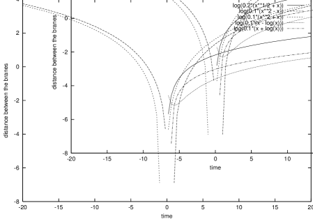
Figure 2: The proper distance between the branes in the case of $\Gamma=\frac{4}{3}$, $\Gamma=\frac{2}{3}$ and $\Gamma=\frac{1}{3}$. Collision moments are regular points.

As pointed out by Kanno and Soda [6] it is possible to recover the 5-dimensional bulk metric from the effective 4-dimensional theory. The 4-dimensional theory works as a hologram and this is the reason to call it holographic brane gravity. Using solutions (12) and (42) we can write the first order of iteration of the 5-dimensional bulk metric as follows ($\Gamma\not=\frac{2}{3}$, $\Gamma\not=0$)

$$g_{\mu\nu}(y,x^{\mu})=(1-\Psi)^{\frac{y}{l}}h_{\mu\nu}(x^{\mu})=\frac{(3\Gamma-2)^{\frac{2y}{l}}}{(9\Gamma^{2}k\lambda_{B}^{0})^{\frac{y}{l}}}\frac{t^{\frac{4}{3\Gamma}}}{\left(t^{\frac{2}{3\Gamma}}\mp t\right)^{\frac{2y}{l}}}f_{ij}(x^{k})\ .$$ (43)

This is a ”brane-based” model of a time dependent bulk geometry which contains two branes with fixed values of $y$-coordinate [14]. Probably it is possible to introduce an alternative ”bulk-based” viewpoint, where the bulk remains static but coordinates of branes are not fixed in respect of a ”bulk-based” coordinate system [4]. Such a model for a one brane model (a domain wall) is treated by Kraus [15]. In both cases the motion of the branes will be interpreted by an observer on a brane as an expansion or a contraction.

4 The influence of the dark radiation

In general, equation (17) is a second order differential equation for scale factor $a(t)$

$$\frac{d^{2}(a^{2})}{dt^{2}}=k\rho_{0}(4-3\Gamma)a^{2-3\Gamma}$$ (44)

and its first integral reads

$$\frac{d(a^{2})}{\sqrt{a^{4-3\Gamma}+\frac{C}{k\rho_{0}}}}=2\sqrt{k\rho_{0}}dt$$ (45)

where $C$ is the constant of integration that is taken to be zero in solutions (23), (34). The missing integration constant can be interpreted as the dark radiation term, which encodes a possible influence of the bulk on the brane. Eq. (45) implies for the Hubble parameter

$$H^{2}=\frac{k\rho_{0}}{a^{3\Gamma}}+\frac{C}{a^{4}}$$ (46)

or, taking into account the conservation law (13)

$$H^{2}=k\rho+\frac{C}{a^{4}}\ .$$ (47)

In the case of vanishing dark radiation we have $C=0$ and eq. (45) determines the same solutions as in the previous section. In the case $\Gamma=0\ ,$ eq. (46) coincides with the expression given by Kanno et al [9].

In the case of nonvanishing dark radiation $C\not=0\ ,$ eq. (45) can easily be integrated only at some special values for $\Gamma$.

1. $\Gamma=0$

$$a^{2}=\frac{1}{2}e^{2\sqrt{k\rho_{0}}(t-t_{0})}-\frac{C}{2k\rho_{0}e^{2\sqrt{k\rho_{0}}(t-t_{0})}}\ .$$ (48)

At late times ($t\rightarrow\infty$) the influence of the dark radiation ($C\not=0$) vanishes and the solution for the scale factor acquires the familiar deSitter form.

2. $\Gamma=\frac{4}{3}$

$$a^{2}=2\sqrt{k\rho_{0}+C}(t-t_{0})\ ,\qquad H=\frac{1}{2\sqrt{t-t_{0}}}\ .$$ (49)

We see that in the case of pure radiation matter tensor the dark radiation has no influence on the Hubble parameter of the A-brane.

3. $\Gamma=\frac{2}{3}$

$$a^{2}=k\rho_{0}(t-t_{0})^{2}-\frac{C}{k\rho_{0}}\ ,\qquad H=\frac{k\rho_{0}(t-t_{0})}{a^{2}}\ .$$ (50)

4. $\Gamma=1$

$$a=\frac{1}{2}\beta^{\frac{1}{3}}+2C^{2}\beta^{-\frac{1}{3}}+C\ ,\qquad\beta=9(k\rho_{0})^{4}(t-t_{0})^{2}-8C^{3}$$

$$+3\sqrt{9(k\rho_{0})^{8}(t-t_{0})^{4}-16C^{3}(k\rho_{0})^{4}(t-t_{0})^{2}}\ .$$ (51)

Let us now investigate constraint (18). Upon substituting value of $k\rho$ (47) we get an equation for $\chi\equiv\sqrt{1-\Psi}$ analogous to eq. (36)

$$\dot{\chi}+H\chi\mp 2\sqrt{k\lambda^{B}_{0}\chi^{4}+\frac{C}{a^{4}}}=0\ .$$ (52)

For a numerical investigation of $\Psi$ constraint (18) can be used in the following form

$$\frac{k\rho_{0}}{a^{3\Gamma}}\frac{(1-\Psi)}{\Psi}-H\frac{{\dot{\Psi}}}{\Psi}+\frac{{\dot{\Psi}}^{2}}{4\Psi(1-\Psi)}-k\lambda^{B}_{0}\frac{(1-\Psi)^{2}}{\Psi}=\frac{C}{a^{4}}$$ (53)

where $H$ and $a$ are determined by eq. (45).

5 Discussion and Summary

In this paper we considered a cosmological scenario where two branes are moving and colliding in a 5-dimensional bulk spacetime. We used a low energy effective theory which is a scalar-tensor type theory on both branes with a specific coupling function. The matter is described by a barotropic perfect fluid on the A-brane and by a phenomenological time dependent “cosmological constant” on the B-brane. We found some special solutions for the scale factor on the A-brane and for the radion which determines the proper distance between the branes.

We conclude that for all values of the barotropic index $\Gamma$, at late time the dynamics on the A-brane is well described by the Einstein general relativity with $\Psi\approx 1$. In the case of a phenomenological cosmological constant on the A-brane ($\Gamma=0,p=-\rho$) we have the deSitter type evolution at late time. This feature seems to be typical also in other braneworld scenarios discussed recently [16] and fits well with the experimental evidence of late time acceleration. Compared with the phenomenological theory (quintessence) the braneword model gives a more motivated theoretical ground to this result.

In the case $\Gamma\not=0$ we first have assumed the power law evolution. This type of solution lacks at least one integration constant which encodes the influence of the bulk (dark radiation on the brane). As a result the cosmological evolution of our Universe on the A-brane coincides with the familiar FRW model and consequently shares all its observational evidences. But this also means that the solution contains no additional hints for approving the braneworld model. Such hints could be found in the explicit solutions with the dark radiation term ($C\not=0$) presented by us in special cases of barotropic index $\Gamma=0,\ 4/3,\ 2/3,\ 1$.

The dynamics of the radion is discussed in detail. We conclude that the collision of the branes can take place at a distinct moment determined by matter tensors on the branes. The evolution of the scale factor and the radion field is regular at the moment of collision. However, we have chosen a very specific coordinate system ([6]) and we have not discussed any other choice. The coordinate effects must be separated from the physical ones and this will be a prospect for a future work.

ACKNOWLEDGMENTS

This work was supported by the Estonian Science Foundation under grants Nos 5026 and 4515.

References

- [1] L. Randall and R. Sundrum, Phys. Rev. Lett. 83, 3370 (1999).
- [2] L. Randall and R. Sundrum, Phys. Rev. Lett. 83, 4690 (1999).
- [3] P. Binetruy, C. Deffayet, and D. Langlois, Nucl. Phys. B565 (2000), 269.
- [4] D. Langlois, Prog. Theor. Phys. Suppl. 148 181, (2003).
- [5] S. Kanno and J. Soda, Phys. Rev. D66, 043526 (2002).
- [6] S. Kanno and J. Soda, Phys. Rev. D66, 083506 (2002).
- [7] J. Khoury, B.A. Ovrut, P.J. Steinhardt, and N. Turok, Phys. Rev. D64, 123522 (2001).
- [8] P. Kuusk and M. Saal, Gen. Rel. Grav. 34, 2135 (2002).
- [9] S. Kanno, M. Sasaki, and J. Soda, Prog. Theor. Phys. 109, 357 (2003).
- [10] M. Gasperini and G. Veneziano, Astropart. Phys. 1, 317 (1993).
- [11] A collection of papers on the pre-big bang scenario is available at homepage http://www.to.infn.it/~gasperin/.
- [12] A. Serena, J.M. Alimi, and A. Navarro, Class. Quant. Grav. 19, 857 (2002).
- [13] I.M. Khalatnikov and A.Yu. Kamenshchik, Class. Quant. Grav. 19, 3845 (2002).
- [14] N. Kaloper, Phys. Rev. D60, 123506 (1999).
- [15] P. Kraus, J. High Energy Phys. 9912 (1999) 011.
- [16] S. Nojiri and S.D. Odintsov, Phys. Lett B565, 1 (2003).