Asymptotic Regimes of Magnetic Bianchi Cosmologies
Joshua T. Horwood and John Wainwright

Abstract. We consider the asymptotic dynamics of the Einstein-Maxwell field equations for the class of non-tilted Bianchi cosmologies with a barotropic perfect fluid and a pure homogeneous source-free magnetic field, with emphasis on models of Bianchi type VII₀, which have not been previously studied. Using the orthonormal frame formalism and Hubble-normalized variables, we show that, as is the case for the previously studied class A magnetic Bianchi models, the magnetic Bianchi VII₀ cosmologies also exhibit an oscillatory approach to the initial singularity. However, in contrast to the other magnetic Bianchi models, we rigorously establish that typical magnetic Bianchi VII₀ cosmologies exhibit the phenomena of asymptotic self-similarity breaking and Weyl curvature dominance in the late-time regime.
Key words. Non-tilted magnetic Bianchi cosmologies.

1 Introduction

The influence of an intergalactic magnetic field on cosmological models has been investigated for over four decades both from a theoretical and observational point of view. Cosmologists speculate that such a field could be primordial in origin, that is, one that came into existence at the Planck time. Observational techniques rely on studying processes such as the temperature distribution of the cosmic microwave background radiation (CMBR), primeval nucleosynthesis and the Faraday rotation of linearly polarized radiation emitted from extragalactic radio sources. Barrow et al [1] derive an upper bound of $B_{0}<3.4\times 10^{-9}\,(\Omega_{0}h_{50}^{2})^{1/2}\,\mathrm{gauss}$ on the present strength of any spatially homogeneous primordial magnetic field based on data from the COBE satellite ($\Omega_{0}$ is the present value of the density parameter and $h_{50}$ is the Hubble constant in units of $50\,\mathrm{km\,s^{-1}\,Mpc^{-1}}$). All observations to date only place an upper bound on the strength of such a magnetic field and hence are inconclusive as regards its existence.

Any cosmological model which contains a magnetic field is necessarily anisotropic, since isotropy is violated by the preferred direction of the magnetic field vector. Consequently, one must analyze the Einstein field equations in models more general than the homogeneous and isotropic Friedmann-Lemaître (FL) models. The simplest family of cosmological models that can admit a magnetic field are the so-called Bianchi cosmologies, that is, models which admit a three-parameter group of isometries acting orthogonally transitively on spacelike hypersurfaces. The models are thus spatially homogeneous, but, in general, anisotropic. We assume that the models contain a barotropic perfect fluid whose four-velocity is orthogonal to the group orbits, and that observers comoving with the fluid measure a pure source-free magnetic field. We also assume that the perfect fluid satisfies an equation of state $p=(\gamma-1)\mu$, where $\gamma$ is constant and satisfies $\frac{2}{3}<\gamma<2$, the cases $\gamma=1$ (dust) and $\gamma=\frac{4}{3}$ (radiation) being of primary interest. We shall refer to solutions of the combined Einstein-Maxwell field euqations that satisfy the above properties as magnetic Bianchi cosmologies. It is known that the field equations lead to restrictions on the Bianchi-Behr type of the isometry group, namely, that it is of types I, II, VI₀ or VII₀ (in class A) or type III (in class B).

Significant progress has been made in the study of magnetic Bianchi cosmologies. Collins [2] was the first to use techniques from dynamical systems theory to obtain qualitative results concerning the evolution of axisymmetric Bianchi I models under the assumption that the magnetic field is aligned along a shear eigenvector. More recently, LeBlanc et al [8] gave a qualitative analysis of the dynamics of magnetic Bianchi cosmologies of type VI₀ in their asymptotic regimes, that is, near the initial singularity and at late times. This work made use of the orthonormal frame formalism of Ellis and MacCallum [4] and Hubble-normalized variables (see [19], ch. 5 and 6). This formalism was also used in [6] and [7] to give a similar analysis of magnetic Bianchi universes of types I and II. Most recently, Crowe [3] extended the results to magnetic Bianchi models of type III. There remains one class which has not been previously analyzed, namely magnetic Bianchi cosmologies of type VII₀.

Our goal in this paper is to fill this gap by giving a qualitative analysis of the dynamics of magnetic Bianchi cosmologies of type VII₀ in their asymptotic regimes. Bianchi cosmologies of type VII₀ are of interest because they represent anisotropic generalizations of the flat FL models. The asymptotic dynamics of the non-magnetic models at late times has only been analyzed in detail relatively recently (see [20]). It is worth comparing non-magnetic Bianchi cosmologies of group type VII₀ with their counterparts of group type I, which are also anisotropic generalizations of the flat FL models. The non-magnetic Bianchi type I cosmologies are asymptotically self-similar at late times, that is, they are approximated by a self-similar solution at late times. This self-similar solution is in fact the flat FL solution, which means that the Bianchi I cosmologies undergo asymptotic isotropization. In contrast, for values of the equation of state parameter $\gamma$ satisfying $\frac{2}{3}<\gamma<2$, the Bianchi VII₀ cosmologies are not asymptotically self-similar at late times. Nevertheless, for values of $\gamma$ satisying $1\leqslant\gamma\leqslant\frac{4}{3}$, they undergo a subtle form of isotropization: the rate of expansion isotropizes, but the intrinsic gravitational field, as described by the Weyl curvature tensor, does not. This phenomenon has been referred to as Weyl curvature dominance (see [20]). One of our specific goals in this paper is to determine what effect a cosmic magnetic field has on the above-mentioned isotropization. The method that we use is a generalization of the analysis of the non-magnetic Bianchi VII₀ and VIII models given in [20] and [5], respectively.

The plan of paper is as follows. In section 2, we present the evolution equations for the magnetic Bianchi cosmologies of type VII₀ using the orthonormal-frame formalism and Hubble-normalized variables. Section 3 contains the main result concerning the dynamics in the late-time regime, namely theorem 3.5 and corollary 3.1, which give the limits of the Hubble-normalized variables and of certain physical dimensionless scalars, thereby describing the asymptotic dynamics at late times. In section 4, we examine the singular asymptotic regime and show that typical models exhibit an oscillatory singularity. We conclude in section 5 with a discussion of the cosmological implications of our results and give an overview of the asymptotic dynamics of the magnetic Bianchi cosmologies, noting that the present paper completes the picture.

There are three appendices. Appendix A contains the proof of the fact that magnetic Bianchi VII₀ universes are not asymptotically self-similar at late times. Appendix B fills in some of the technical details of the proof of theorem 3.5. Finally, in appendix C we give expressions for a dimensionless scalar formed from the Weyl curvature tensor in terms of the Hubble-normalized variables.

2 Evolution equations

In this section we give the evolution equations for magnetic Bianchi cosmologies of type VII₀. As described in [8] (pg. 517), we use Hubble-normalized variables

$$(\Sigma_{+},\Sigma_{-},N_{2},N_{3},\mathcal{H}),$$ (2.1)

defined relative to a group-invariant orthonormal frame $\{\boldsymbol{e}_{a}\}$, with $\boldsymbol{e}_{0}=\boldsymbol{u}$, the fluid 4-velocity, which is normal to the group orbits.

The variables $\Sigma_{\pm}$ describe the shear of the fluid congruence, the $N_{2,3}$ are spatial connection variables which describe the intrinsic curvature of the group orbits and the variable $\mathcal{H}$ describes the magnetic degree of freedom. The magnetic Bianchi VII₀ cosmologies are described by the inequalities $\mathcal{H}>0$ and $N_{2}N_{3}>0$. Without loss of generality, we assume

$$N_{2}>0,\qquad N_{3}>0.$$ (2.2)

It is convenient to define

$$N_{+}={\textstyle\frac{1}{2}}(N_{2}+N_{3}),\qquad N_{-}={\textstyle\frac{1}{2\sqrt{3}}}(N_{2}-N_{3}),$$ (2.3)

and replace (2.1) by the state vector

$$(\Sigma_{+},\Sigma_{-},N_{+},N_{-},\mathcal{H}).$$ (2.4)

The restrictions (2.2) become

$$N_{+}>0,\qquad N_{+}^{2}-3N_{-}^{2}>0,\qquad\mathcal{H}>0.$$ (2.5)

The state variables (2.1) and (2.4) are dimensionless, having been normalized with the Hubble scalar $H$, which is related to the overall length scale $\ell$ by

$$H=\frac{\dot{\ell}}{\ell},$$ (2.6)

where the overdot denotes differentiation with respect to clock time along the fundamental congruence. The state variables depend on a dimensionless time variable $\tau$ that is related to the length scale $\ell$ by

$$\ell=\ell_{0}\,\mathrm{e}^{\tau},$$ (2.7)

where $\ell_{0}$ is a constant. The dimensionless time $\tau$ is related to the clock time $t$ by

$$\frac{\mathrm{d}t}{\mathrm{d}\tau}=\frac{1}{H},$$ (2.8)

as follows from equations (2.6) and (2.7). In formulating the evolution equations we require the deceleration parameter $q$, defined by

$$q=-\frac{\ell\ddot{\ell}}{\dot{\ell}^{2}},$$ (2.9)

and the density parameter $\Omega$, defined by

$$\Omega=\frac{\mu}{3H^{2}}.$$ (2.10)

We also find it convenient to introduce the magnetic density parameter $\Omega_{h}$, defined analogously by

$$\Omega_{h}=\frac{\mu_{h}}{3H^{2}},$$ (2.11)

where $\mu_{h}$ is the energy density of the magnetic field. We note that $\mu_{h}$ is given by

$$\mu_{h}={\textstyle\frac{1}{2}}(h_{1}^{2}+h_{2}^{2}+h_{3}^{2}),$$ (2.12)

where the $h_{\alpha}$, $\alpha=1,2,3$, are the components of the magnetic field intensity relative to the spatial orthonormal frame $\{\boldsymbol{e}_{\alpha}\}$, which has been chosen so that

$$h_{\alpha}=(h_{1},0,0)$$ (2.13)

(see [8]).

A complete derivation of the evolution equations for the variables (2.4), which arise from the combined Einstein-Maxwell field equations, is provided in [8] (see section 2). These evolution equations read

$$\begin{split}\Sigma^{\prime}_{+}&=(q-2)\Sigma_{+}-2N_{-}^{2}+{\textstyle\frac{1}{3}}\mathcal{H}^{2},\\ \Sigma^{\prime}_{-}&=(q-2)\Sigma_{-}-2N_{+}N_{-},\\ N^{\prime}_{+}&=(q+2\Sigma_{+})N_{+}+6\Sigma_{-}N_{-},\\ N^{\prime}_{-}&=(q+2\Sigma_{+})N_{-}+2\Sigma_{-}N_{+},\\ \mathcal{H}^{\prime}&=(q-2\Sigma_{+}-1)\mathcal{H},\end{split}$$ (2.14)

where

$$q =2(\Sigma_{+}^{2}+\Sigma_{-}^{2})+{\textstyle\frac{1}{6}}\mathcal{H}^{2}+{\textstyle\frac{1}{2}}(3\gamma-2)\Omega,$$ (2.15)

$$\Omega =1-\Sigma_{+}^{2}-\Sigma_{-}^{2}-N_{-}^{2}-{\textstyle\frac{1}{6}}\mathcal{H}^{2},$$ (2.16)

and ^′ denotes differentiation with respect to $\tau$. For future reference we also note the evolution equation for $\Omega$:

$$\Omega^{\prime}=[2q-(3\gamma-2)]\Omega,$$ (2.17)

and the expression for the magnetic density parameter

$$\Omega_{h}={\textstyle\frac{1}{6}}\mathcal{H}^{2},$$ (2.18)

in terms of the Hubble-normalized magnetic field intensity $\mathcal{H}=h_{1}/H$, which follows from (2.11), (2.12) and (2.13).

The physical requirement $\Omega\geqslant 0$ in conjunction with (2.3) implies that the variables $\Sigma_{\pm}$, $N_{-}$ and $\mathcal{H}$ are bounded, but places no restriction on $N_{+}$ itself. In fact, it will be shown in appendix A (see proposition A.1) that if $\Omega>0$ and $\frac{2}{3}<\gamma<2$, then for any initial conditions

$$\lim_{\tau\rightarrow+\infty}N_{+}=+\infty.$$ (2.19)

The first step in analyzing the dynamics at late times ($\tau\rightarrow+\infty$) is to introduce new variables which are bounded at late times and which enable us to isolate the oscillatory behaviour associated with $\Sigma_{-}$ and $N_{-}$. Motivated by [20], we define

$$\Sigma_{-}=R\cos\psi,\qquad N_{-}=R\sin\psi,\qquad M=\frac{1}{N_{+}},$$ (2.20)

where $R\geqslant 0$.

In terms of the new variables $(\Sigma_{+},R,\mathcal{H},M,\psi)$, the evolution equations (2.14) have the following form

$$\begin{split}\Sigma^{\prime}_{+}&=(Q-2)\Sigma_{+}-R^{2}+{\textstyle\frac{1}{3}}\mathcal{H}^{2}+(1+\Sigma_{+})R^{2}\cos 2\psi,\\ R^{\prime}&=\left[Q+\Sigma_{+}-1+(R^{2}-1-\Sigma_{+})\cos 2\psi\right]R,\\ \mathcal{H}^{\prime}&=\left[Q-2\Sigma_{+}-1+R^{2}\cos 2\psi\right]\mathcal{H},\\ M^{\prime}&=-\left[Q+2\Sigma_{+}+R^{2}(\cos 2\psi+3M\sin 2\psi)\right]M,\\ \psi^{\prime}&=\frac{1}{M}\left[2+(1+\Sigma_{+})M\sin 2\psi\right],\end{split}$$ (2.21)

where

$$Q=2\Sigma_{+}^{2}+R^{2}+{\textstyle\frac{1}{6}}\mathcal{H}^{2}+{\textstyle\frac{1}{2}}(3\gamma-2)\Omega,$$ (2.22)

and

$$\Omega=1-\Sigma_{+}^{2}-R^{2}-\Omega_{h}.$$ (2.23)

The evolution equation for $\Omega$ becomes

$$\Omega^{\prime}=\left[2Q-(3\gamma-2)+2R^{2}\cos 2\psi\right]\Omega.$$ (2.24)

The restrictions (2.5) are equivalent to

$$3M^{2}R^{2}\sin^{2}\psi<1,\qquad M>0,\qquad R\geqslant 0,\qquad\mathcal{H}>0.$$ (2.25)

3 Limits at late times

In this section we present a theorem which gives the limiting behaviour as $\tau\rightarrow+\infty$ of the magnetic Bianchi VII₀ cosmologies when the equation of state parameter $\gamma$ satisfies $\frac{2}{3}<\gamma<2$. As a corollary of the theorem, we obtain the limiting behaviour of certain dimensionless scalars that describe physical properties of the models, namely the density parameter $\Omega$, defined by (2.10), the magnetic density parameter $\Omega_{h}$, defined by (2.11), the shear parameter $\Sigma$, defined by

$$\Sigma^{2}=\frac{\sigma_{ab}\sigma^{ab}}{6H^{2}},$$ (3.1)

where $\sigma_{ab}$ is the rate-of-shear tensor of the fluid congruence, and the Weyl curvature parameter $\mathcal{W}$, defined by

$$\mathcal{W}^{2}=\frac{E_{ab}E^{ab}+H_{ab}H^{ab}}{6H^{4}},$$ (3.2)

where $E_{ab}$ and $H_{ab}$ are the electric and magnetic parts of the Weyl tensor, respectively (see [19], pg. 19), relative to the fluid congruence.

In terms of the Hubble-normalized variables, the shear parameter is given by

$$\Sigma^{2}=\Sigma_{+}^{2}+R^{2}\cos^{2}\psi,$$ (3.3)

which follows from (2.20) in conjunction with equation (6.13) in [19]. The formula for the Weyl curvature parameter is more complicated and is provided in appendix C.

The main result concerning the limits of $\Sigma_{+}$, $R$, $\mathcal{H}$ and $M$ is contained in the following theorem. Some of the results depend on requiring that the model is not locally rotationally symmetric (LRS).

Theorem 3.1.

For all magnetic Bianchi cosmologies of type VII₀ that are not LRS and with density parameter $\Omega$ satisfying $\Omega>0$, the Hubble-normalized state variables $(\Sigma_{+},R,\mathcal{H},M)$ satisfy

$$\lim_{\tau\rightarrow+\infty}(\Sigma_{+},R,\mathcal{H},M)=\begin{cases}(0,0,0,0),&\text{if}\quad\frac{2}{3}<\gamma<\frac{4}{3},\\ \left(0,\sqrt{{\textstyle\frac{2}{3}}}\,k,\sqrt{2}\,k,0\right),&\text{if}\quad\gamma=\frac{4}{3},\\ \left(0,\sqrt{{\textstyle\frac{2}{3}}},\sqrt{2},0\right),&\text{if}\quad\frac{4}{3}<\gamma<2,\end{cases}$$ (3.4)

and

$$\lim_{\tau\rightarrow+\infty}\frac{M}{R}=\begin{cases}+\infty,&\text{if}\quad\frac{2}{3}<\gamma<1,\\ L\not=0,&\text{if}\quad\gamma=1,\\ 0,&\text{if}\quad 1<\gamma<2,\end{cases}$$ (3.5)

where $k\in(0,1)$ and $L>0$ are constants that depend on the initial conditions.

Proof. It follows immediately from (2.19) and (2.20) that

$$\lim_{\tau\rightarrow+\infty}M=0.$$ (3.6)

Furthermore, since $\Sigma_{+}$ is bounded, it follows from the $\psi$ evolution equation in (2.21) that

$$\lim_{\tau\rightarrow+\infty}\psi=+\infty.$$ (3.7)

The trigonometric functions in the DE (2.21) thus oscillate increasing rapidly as $\tau\rightarrow+\infty$. In order to control these oscillations, we introduce new gravitational variables $\bar{\Sigma}_{+}$, $\bar{R}$ and $\bar{\mathcal{H}}$ according to

$$\begin{split}\bar{\Sigma}_{+}&=\Sigma_{+}-{\textstyle\frac{1}{4}}(1+\Sigma_{+})R^{2}M\sin 2\psi,\\ \bar{R}&=R\left[1-{\textstyle\frac{1}{4}}(R^{2}-1-\Sigma_{+})M\sin 2\psi\right],\\ \bar{\mathcal{H}}&=\mathcal{H}\left[1-{\textstyle\frac{1}{4}}R^{2}M\sin 2\psi\right].\end{split}$$ (3.8)

These new variables are defined so as to ‘suppress’ the rapidly oscillating terms which may not tend to zero as $\tau\rightarrow+\infty$. The evolution equations for these “barred” variables, which can be derived from (2.21) and (3.8), have the following form

$$\begin{split}\bar{\Sigma}^{\prime}_{+}&=-(2-\bar{Q})\bar{\Sigma}_{+}-\bar{R}^{2}+{\textstyle\frac{1}{3}}\bar{\mathcal{H}}^{2}+MB_{\bar{\Sigma}_{+}},\\ \bar{R}^{\prime}&=(\bar{Q}+\bar{\Sigma}_{+}-1+MB_{\bar{R}})\bar{R},\\ \bar{\mathcal{H}}^{\prime}&=(\bar{Q}-2\bar{\Sigma}_{+}-1+MB_{\bar{\mathcal{H}}})\bar{\mathcal{H}},\end{split}$$ (3.9)

where

$$\bar{Q}=2\bar{\Sigma}_{+}^{2}+\bar{R}^{2}+{\textstyle\frac{1}{6}}\bar{\mathcal{H}}^{2}+{\textstyle\frac{1}{2}}(3\gamma-2)\left(1-\bar{\Sigma}_{+}^{2}-\bar{R}^{2}-{\textstyle\frac{1}{6}}\bar{\mathcal{H}}^{2}\right),$$ (3.10)

and the $B$ terms are bounded functions in $\bar{\Sigma}_{+}$, $\bar{R}$, $\bar{\mathcal{H}}$ and in $M$ and $\psi$ for $\tau$ sufficiently large. The essential idea is to regard $M$ and $\psi$ as arbitrary functions of $\tau$ subject only to (3.6). Thus, (3.9) is a non-autonomous DE for

$$\bar{\boldsymbol{x}}=(\bar{\Sigma}_{+},\bar{R},\bar{\mathcal{H}}),$$

of the form

$$\bar{\boldsymbol{x}}^{\prime}=\boldsymbol{f}(\bar{\boldsymbol{x}})+\boldsymbol{g}(\bar{\boldsymbol{x}},\tau),$$ (3.11)

where

$$\boldsymbol{g}(\bar{\boldsymbol{x}},\tau)=M(\tau)(B_{\bar{\Sigma}_{+}},\bar{R}B_{\bar{R}},\bar{\mathcal{H}}B_{\bar{\mathcal{H}}}),$$ (3.12)

and $\boldsymbol{f}(\bar{\boldsymbol{x}})$ can be read off from the right-hand side of (3.9). Since

$$\lim_{\tau\rightarrow+\infty}\boldsymbol{g}(\bar{\boldsymbol{x}},\tau)=\mathbf{0},$$

as follows from (3.6), the DE (3.9) is asymptotically autonomous (see [12]). The corresponding autonomous DE is

$$\hat{\boldsymbol{x}}=\boldsymbol{f}(\hat{\boldsymbol{x}}),$$ (3.13)

where

$$\hat{\boldsymbol{x}}=(\hat{\Sigma}_{+},\hat{R},\hat{\mathcal{H}}).$$

Using standard methods from the theory of dynamical systems, we first show that the limits of the “hatted” variables correspond to those limits stated in the theorem. Details are provided in appendix B.1. We then use a theorem from [12] (see theorem B.1 in appendix B) to infer that the solutions of the non-autonomous DE (3.11) have the same limits as the solutions of the autonomous DE (3.13). Details are provided in appendix B.2. The limit of $\boldsymbol{x}=(\Sigma_{+},R,\mathcal{H})$ follows immediately from this result in conjunction with the definitions (3.8). Finally, the limit (3.5) concerning the ratio $M/R$ is obvious when $\frac{4}{3}\leqslant\gamma<2$, since $R\nrightarrow 0$. The more complicated case when $\frac{2}{3}<\gamma<\frac{4}{3}$ is treated in appendix B.3. $\Box$

Table 1: Limits of the Hubble-normalized scalars $\Omega$, $\Omega_{h}$, $\Sigma$ and $\mathcal{W}$ at late times for magnetic Bianchi cosmologies of type VII₀.

Range of $\gamma$	$\Omega$	$\Omega_{h}$	$\Sigma^{2}$	$\mathcal{W}$
$\frac{2}{3}<\gamma<1$	1	0	0	0
$\gamma=1$	1	0	0	$L\not=0$
$1<\gamma<\frac{4}{3}$	1	0	0	$+\infty$
$\gamma=\frac{4}{3}$	$1-k^{2}$	$\frac{1}{3}k^{2}$	$\left(0,\frac{2}{3}k^{2}\right)$	$+\infty$
$\frac{4}{3}<\gamma<2$	0	$\frac{1}{3}$	$\left(0,\frac{2}{3}\right)$	$+\infty$

Corollary 3.1.

The limits as $\tau\rightarrow+\infty$ of the density parameter $\Omega$, the magnetic density parameter $\Omega_{h}$, the shear scalar $\Sigma$ and the Weyl curvature scalar $\mathcal{W}$, for all magnetic Bianchi cosmologies of type VII₀ that are not LRS and with $\Omega$ satisfying $\Omega>0$, are as given in table 1.

Proof. These results follow directly from theorem 3.5 and equations (2.23), (3.3), (C.3) and (C.4). Moreover, if $1<\gamma<2$, it follows from (C.3) and (C.4) that since $\Sigma_{+}$, $R$ and $\mathcal{H}$ are bounded, and $\lim_{\tau\rightarrow+\infty}M/R=0$, that

$$\mathcal{W}=\frac{2R}{M}[1+\mathcal{O}(M)],$$

as $\tau\rightarrow+\infty$. $\Box$

We conclude this section by discussing the physical interpretations of theorem 3.5 and its corollary. Like the non-magnetic Bianchi VII₀ models, the magnetic Bianchi VII₀ models are not asymptotically self-similar at late times, since the orbits in the Hubble-normalized state space do not approach an equilibrium point of the evolution equations. This phenomenon is accompanied by Weyl curvature dominance, characterized by the divergence of the Weyl curvature scalar $\mathcal{W}$ which describes the intrinsic anisotropy of the gravitational field. For non-LRS models with $1<\gamma<2$, $\mathcal{W}$ is unbounded as $\tau\rightarrow+\infty$.

The shear scalar $\Sigma$ quantifies the anisotropy in the expansion of a cosmological model. We see that for $\frac{2}{3}<\gamma<\frac{4}{3}$, the models isotropize at late times in the sense that $\lim_{\tau\rightarrow+\infty}\Sigma=0$, as is the case for the corresponding non-magnetic Bianchi VII₀ models (see [20], theorem 2.3). The key difference between the magnetic and non-magnetic models occurs when the matter content is a radiation fluid ($\gamma=\frac{4}{3}$): the presence of a magnetic field prevents shear isotropization, in the sense that $\Sigma$ does not tend to zero at late times.

4 The singular asymptotic regime

In this section we show, by combining numerical experiments with analytical considerations, that generic non-LRS magnetic Bianchi VII₀ cosmologies with $\frac{2}{3}<\gamma<2$ exhibit an oscillatory approach to the initial singularity, as do the other class A magnetic Bianchi models.

Figure 1: The arrays $-++$, etc. give the signs of the eigenvalues $\lambda_{\mathcal{H}}$, $\lambda_{N_{2}}$ and $\lambda_{N_{3}}$ in that order. The variables listed next to each of the three arcs indicates which of the variables $\mathcal{H}$, $N_{2,3}$ is growing into the past.

As is the case for the previously studied class A magnetic Bianchi models, the behaviour into the past for the magnetic Bianchi VII₀ models is necessarily complicated since none of the equilibrium points of the evolution equations (2.14) are local sources. It is well-known that in the dynamical systems approach, the Kasner circle $\mathcal{K}$ plays a primary role in determining the dynamics towards the singularity, since its local stability enables one to predict whether the singularity in a given class of models is oscillatory. For the present class of models, $\mathcal{K}$ is the set of equilibrium points described by

$$\Sigma_{+}^{2}+\Sigma_{-}^{2}=1,\qquad N_{2}=N_{3}=\mathcal{H}=0.$$

A local stability analysis shows that the Kasner equilibrium points are saddles in the Hubble-normalized state space. Apart from three exceptional points (labeled $T_{1}$, $T_{2}$ and $T_{3}$ in figure 1), the equilibrium points of $\mathcal{K}$ have a one-dimensional unstable manifold into the past. Figure 1 shows the signs of the eigenvalues on $\mathcal{K}$ associated with the variables $\mathcal{H}$, $N_{2}$ and $N_{3}$ (a negative eigenvalue indicates instability into the past) and which of these three variables are increasing into the past in a neighbourhood of the Kasner circle.

It turns out each unstable manifold on $\mathcal{K}$ is asymptotic to another Kasner point. In other words, the unstable manifold is a heteroclinic orbit of $\mathcal{K}$, i.e. an orbit which joins two Kasner points. These unstable manifolds provide a mechanism for a cosmological model to make a transition from one (approximate) Kasner state to another, as it evolves into the past. Figure 2 shows the projections in the $\Sigma_{+}\Sigma_{-}$-plane, of these families of heteroclinic orbits, that join two Kasner points. The families are described as follows:

$$\begin{array}[]{llll}\mathcal{S}_{\mathcal{H}}:&\quad\Sigma_{+}^{2}+\Sigma_{-}^{2}+{\textstyle\frac{1}{6}}\mathcal{H}^{2}=1,&\quad\mathcal{H}>0,&\quad N_{2}=N_{3}=0,\\ \mathcal{S}_{N_{2}}:&\quad\Sigma_{+}^{2}+\Sigma_{-}^{2}+{\textstyle\frac{1}{12}}N_{2}^{2}=1,&\quad N_{2}>0,&\quad N_{3}=\mathcal{H}=0,\\ \mathcal{S}_{N_{3}}:&\quad\Sigma_{+}^{2}+\Sigma_{-}^{2}+{\textstyle\frac{1}{12}}N_{3}^{2}=1,&\quad N_{3}>0,&\quad N_{2}=\mathcal{H}=0.\end{array}$$ (4.1)

The heteroclinic orbits on $\mathcal{S}_{N_{2,3}}$ describe the familiar vacuum Bianchi II Taub models, while the orbits on $\mathcal{S}_{\mathcal{H}}$ describe the Rosen magneto-vacuum models (see [8], pg. 531).

Numerical experiments suggest that for generic non-LRS models, after an initial transient stage, the orbit approaches a point on $\mathcal{K}$. The direction of departure of the orbit is determined by the unique Rosen or Taub orbit through that point whereupon it shadows (i.e. is approximated by) this orbit until is approaches another point on $\mathcal{K}$ and the process repeats indefinitely. In physical terms, the corresponding cosmological model is approximated by an infinite sequence of Kasner vacuum models as the singularity is approached into the past, the so-called Mixmaster oscillatory singularity. This behaviour motivates the following conjecture concerning the past attractor $\mathcal{A}^{-}$.

$\mathcal{S}_{\mathcal{H}}$	$\mathcal{S}_{N_{2}}$	$\mathcal{S}_{N_{3}}$

Figure 2: The projections of the Rosen and Taub orbits joining points on the Kasner circle $\mathcal{K}$. The arrows show evolution into the past.

Conjecture 4.1.

The past attractor is the two-dimensional invariant set consisting of all orbits in the invariant sets $\mathcal{S}_{\mathcal{H}}$, $\mathcal{S}_{N_{2}}$ and $\mathcal{S}_{N_{3}}$ (see figure 2) and the Kasner equilibrium points, i.e.

$$\mathcal{A}^{-}=\mathcal{S}_{\mathcal{H}}\cup\mathcal{S}_{N_{2}}\cup\mathcal{S}_{N_{3}}\cup\mathcal{K}.$$ (4.2)

This conjecture can be formulated in terms of limits of the state variables as follows. Referring to (2.16) and (4.1), we see that the set $\mathcal{A}^{-}$ is defined by $\Omega=0$ and

$$N_{2}\mathcal{H}=N_{3}\mathcal{H}=N_{2}N_{3}=0.$$

It follows from monotone function arguments (see the comment at the end of appendix A) that

$$\lim_{\tau\rightarrow-\infty}N_{2}N_{3}=0,$$

and, moreover, that $N_{2}$ and $N_{3}$ are bounded in the singular regime. Thus our conjecture concerning the past attractor can be formulated as

$$\lim_{\tau\rightarrow-\infty}\Omega=0,\qquad\lim_{\tau\rightarrow-\infty}N_{2}\mathcal{H}=0,\qquad\lim_{\tau\rightarrow-\infty}N_{3}\mathcal{H}=0.$$

Note that for a generic orbit, $\lim_{\tau\rightarrow-\infty}(\mathcal{H},N_{2},N_{3})$ does not exist.

5 Discussion

With the appearance of the present paper there is now available a complete description of the dynamics of magnetic Bianchi cosmologies with a perfect-fluid matter content, in the two asymptotic regimes. We now give an overview of the properties of these models, in order to highlight the role of a primordial magnetic field in spatially homogeneous cosmological dynamics. The possible Bianchi types and relevant references are given in the introduction. We emphasize the so-called class A models (in the terminology of Ellis and MacCallum [4]), that is, those of Bianchi types I, II, VI₀ and VII₀. For each of these types the Hubble-normalized state space is five-dimensional, but, as indicated in table 2, they differ as regards the number of degrees of freedom associated with spatial curvature and with the magnetic field. In this table we have also listed Bianchi types VIII and IX, which do not admit a magnetic field, for comparison purposes.

Table 2: Shear, spatial curvature and magnetic degrees of freedom in class A Bianchi cosmologies.

Bianchi type	Shear	Spatial curvature	Magnetic field
I	2	0	3
II	2	1	2
VI0, VII0	2	2	1
VIII, IX	2	3	0

All models in table 2 display an oscillatory approach to the singularity, described by a two-dimensional attractor in the Hubble-normalized state space, familiar from the non-magnetic Bianchi VIII and IX models (see [19], pp. 143–7). The essential point is that the magnetic field mimics spatial curvature in that it destabilizes the Kasner circle of equilibrium points. Note that the sum of the number of spatial curvature and magnetic degrees of freedom is three, in all cases in table 2.

Table 3: Limiting values of $\Omega$, $\Omega_{h}$, $\Sigma$ and $\mathcal{W}$ as $\tau\rightarrow+\infty$ for magnetic Bianchi cosmologies with a dust fluid ($\gamma=1$).

Bianchi type	$\Omega$	$\Omega_{h}$	$\Sigma^{2}$	$\mathcal{W}^{2}$
I	1	0	0	0
II	$\frac{15}{16}$	0	$\frac{1}{64}$	$\frac{45}{2048}$
VI0	$\frac{3}{4}(1-k^{2})$	$\frac{3}{8}k^{2}$	$\frac{1}{16}$	$\frac{9}{128}(1+2k^{2})(2+k^{2})$
VII0	1	0	0	$L>0$

As regards the late-time dynamics of the magnetic cosmologies, there is a fundamental difference between the Bianchi VII₀ models considered in the present paper and the Bianchi I, II and VI₀ models considered earlier ([8], [6], [7]), as follows. The Bianchi I, II and VI₀ models are asymptotically self-similar, in the sense that each model is approximated by an exact self-similar solution, while the models of type VII₀ are not asymptotically self-similar. This difference is essentially a consequence of the fact that the Hubble-normalized state space of the Bianchi VII₀ models is unbounded. Another feature of the magnetic cosmologies is that the asymptotic dynamics at late times depends significantly on the equation of state parameter $\gamma$. We illustrate this dependence in tables 3 and 4 where we give the limits at late times of $\Omega$, $\Omega_{h}$, $\Sigma$ and $\mathcal{W}$ for the two physically important cases, dust ($\gamma=1$) and radiation ($\gamma=\frac{4}{3}$). It is worthy of note that if $\gamma<\frac{4}{3}$, the Bianchi I models isotropize in all respects ($\Sigma\rightarrow 0$, $\mathcal{W}\rightarrow 0$ and $\Omega_{h}\rightarrow 0$) while the Bianchi VII₀ models isotropize as regards the shear and the magnetic field ($\Sigma\rightarrow 0$ and $\Omega_{h}\rightarrow 0$).

A cosmic magnetic field also affects the local stability of the equilibrium point that corresponds to the flat FL solution. For non-magnetic models, the flat FL equilibrium point is typically a saddle point, having both a non-trivial stable manifold and a non-trivial unstable manifold. The shear degrees of freedom generate the stable manifold while the spatial curvature degrees of freedom generate the unstable manifold. The stable manifold leads to the phenomenon of intermediate isotropization, i.e. a model can evolve to become arbitrarily close to isotropy over a finite interval of time. The unstable manifold leads to models with an isotropic singularity, i.e. models which are highly isotropic near the initial singularity, but which subsequently develop anisotropies. The effect of a primordial magnetic field on these phenomena depends on the equation of state parameter $\gamma$. If $\gamma<\frac{4}{3}$, the magnetic field increases the dimension of the stable manifold, leaving the dimension of the unstable manifold unchanged, thus increasing the likelihood of intermediate isotropization. On the other hand, if $\gamma>\frac{4}{3}$, the magnetic field increases the dimension of the unstable manifold by one, leading to magnetic models with an isotropic singularity.

Table 4: Limiting values of $\Omega$, $\Omega_{h}$, $\Sigma$ and $\mathcal{W}$ as $\tau\rightarrow+\infty$ for magnetic Bianchi cosmologies with a radiation fluid ($\gamma=\frac{4}{3}$).

Bianchi type	$\Omega$	$\Omega_{h}$	$\Sigma^{2}$	$\mathcal{W}^{2}$
I	1	0	0	0
II	$\frac{3}{4}$	$\frac{1}{12}$	$\frac{1}{12}$	$\frac{21}{144}$
VI0	0	$\frac{3}{8}$	$\frac{1}{16}$	$\frac{81}{128}$
VII0	$1-k^{2}$	$\frac{1}{3}k^{2}$	$\left(0,\frac{2}{3}k^{2}\right)$	$+\infty$

We conclude by giving some suggestions for future research. Firstly, it would be of interest to investigate the asymptotic dynamics of spatially inhomogeneous cosmological models in the presence of a primordial magnetic field, in order to determine which features of magnetic Bianchi cosmologies occur in models without symmetries. The recent paper [18] on $G_{0}$ cosmologies would provide a suitable framework for such an investigation. One step has been taken in this direction by Weaver et al [21], who investigated a family of inhomogeneous cosmologies that generalize the magnetic Bianchi VI₀ cosmologies, and provided numerical evidence that the singularity is oscillatory.

Secondly, the work of Barrow et al [1] referred to in the introduction leads to an upper bound on the magnetic density parameter $\Omega_{h}$ of order $10^{-10}$ for spatially homogeneous magnetic fields. It would be of interest to what extent this upper bound would be weakened within the class of spatially inhomogeneous magnetic cosmologies. The analysis of the anisotropies in the CMBR by Maartens et al [9] would probably provide a suitable framework for such an analysis.

We finally comment briefly on other recent work on magnetic fields in cosmology, which has focused on the potential dynamical effects of a primordial magnetic field in a perturbed FL cosmology ([10], [11], [13], [14], [15], [17]), or in a perturbed Bianchi I cosmology ([16]). This work, which makes use of the Ellis-Bruni covariant and gauge-invariant method for analyzing cosmological density perturbations, complements the results in our paper and related ones, which focus on the dynamics in the asymptotic regimes of magnetic Bianchi cosmologies, and on the likelihood that such a model will evolve to be close to FL. Extending the dynamical systems analysis of magnetic Bianchi cosmologies to spatially inhomogeneous magnetic cosmologies may help to bridge the gap between these two bodies of work.

Appendix A

In this appendix we prove (2.19), concerning the limit of the Hubble-normalized variable $N_{+}$ in the late-time regime. This result is restated as proposition A.1 below.

Proposition A.1.

For all magnetic Bianchi cosmologies of type VII₀ that are not LRS, with equation of state parameter $\gamma$ subject to $\frac{2}{3}<\gamma<2$, and density parameter $\Omega$ satisfying $\Omega>0$, the Hubble-normalized variable $N_{+}$ satisfies

$$\lim_{\tau\rightarrow+\infty}N_{+}=+\infty.$$ (A.1)

Proof. The proof is similar to the proof of the corresponding result for non-magnetic Bianchi VII₀ cosmologies (see theorem 2.1 and equation (A.5) in [20]), in that it makes use of monotone functions and the so-called monotonicity principle (see chapter 4 in [19]). There are two cases depending on the value of $\gamma$.

Case 1. $\frac{2}{3}<\gamma\leqslant 1$

As in [20], we consider the function

$$Z_{1}=\frac{(N_{+}^{2}-3N_{-}^{2})^{v}\Omega}{(1+v\Sigma_{+})^{2(1+v)}},$$

with $v=\frac{1}{4}(3\gamma-2)$. The evolution equations (2.14) imply that

$$\frac{Z^{\prime}_{1}}{Z_{1}}=\frac{4[(\Sigma_{+}+v)^{2}+(1-v^{2})\Sigma_{-}^{2}]}{1+v\Sigma_{+}}+\frac{(1+v)(1-4v)\mathcal{H}^{2}}{3(1+v\Sigma_{+})}.$$

Since $0<v\leqslant\frac{1}{4}$ in this case, it follows that $Z_{1}$ is monotone increasing and the result (A.1) follows as in the non-magnetic case (see appendix A in [20]).

Case 2. $1<\gamma<2$

We give a proof by contradiction. Suppose that (A.1) does not hold. Since the remaining variables are bounded, it follows that for any point $\boldsymbol{x}$ in the state space the $\omega$-limit set $\omega(\boldsymbol{x})$ is non-empty.

Consider the function

$$Z_{2}=\frac{\Sigma_{-}^{2}+N_{-}^{2}}{N_{+}^{2}-3N_{-}^{2}},$$ (A.2)

which satisfies $0<Z_{2}<+\infty$ on the invariant set $S$ defined by

$$N_{+}>0,\qquad N_{+}^{2}-3N_{-}^{2}>0,\qquad\Sigma_{-}^{2}+N_{-}^{2}>0,\qquad\Omega\geqslant 0,\qquad\mathcal{H}\geqslant 0.$$ (A.3)

The evolution equations (2.14) imply that

$$\frac{Z^{\prime}_{2}}{Z_{2}}=\frac{-4(1+\Sigma_{+})\Sigma_{-}^{2}}{\Sigma_{-}^{2}+N_{-}^{2}}.$$

It follows that $Z_{2}$ is decreasing along orbits in $S$. We can now apply the monotonicity principle. By (A.3) the set $\bar{S}\setminus S$ (the set of boundary points of $S$ that are not contained in $S$) is defined by one or both of the following equalities holding

$$N_{+}^{2}-3N_{-}^{2}=0,\qquad\Sigma_{-}^{2}+N_{-}^{2}=0.$$ (A.4)

It now follows that for any $\boldsymbol{x}\in S$, the $\omega$-limit set $\omega(\boldsymbol{x})$ is contained in the subset of $\bar{S}\setminus S$ that satisfies $\lim_{\boldsymbol{y}\rightarrow\boldsymbol{s}}Z_{2}(\boldsymbol{y})\not=+\infty$, where $\boldsymbol{s}\in\bar{S}\setminus S$ and $\boldsymbol{y}\in S$. On account of (A.2) and (A.4) we conclude that

$$\omega(\boldsymbol{x})\subset\{\boldsymbol{x}\>|\>\Sigma_{-}=N_{-}=0\}.$$ (A.5)

We can further restrict the possible $\omega$-limit sets by considering the function

$$Z_{3}=\frac{\Omega^{2}}{(N_{+}^{2}-3N_{-}^{2})\mathcal{H}^{2}},$$

which satisfies

$$Z^{\prime}_{3}=-6(\gamma-1)Z_{3},$$

as follows from (2.14). We immediately conclude that $\lim_{\tau\rightarrow+\infty}Z_{3}=0$ and hence that $\lim_{\tau\rightarrow+\infty}\Omega=0$. In conjunction with (A.5), this result implies that $\omega(\boldsymbol{x})\subset S_{1}$, where

$$S_{1}=\{\boldsymbol{x}\>|\>\Sigma_{-}=N_{-}=\Omega=0\}.$$

The only potential $\omega$-limit sets in $S_{1}$ are equilibrium points, since $\lim_{\tau\rightarrow+\infty}N_{+}=+\infty$ for all other orbits in $S_{1}$. The equilibrium points are

• $\Sigma_{+}=1,\quad N_{+}=\mathcal{H}=0,\quad\text{(an isolated point)}$

• $\Sigma_{+}=-1,\quad\mathcal{H}=0,\quad N_{+}>0\quad\text{(a line)}$.

No orbit with $\mathcal{H}>0$, $\Omega>0$ and $1<\gamma<2$ can be future asymptotic to any of these equilibrium points, since $\Omega^{\prime}>0$ in a neighbourhood of any of these points as follows from (2.17) and (2.15). Thus we have a contradiction of the fact that $\omega(\boldsymbol{x})\not=\phi$, and as a result, (A.1) holds in case 2. $\Box$

Comment. The monotone function (A.2) also provides useful information about the past asymptotics of magnetic Bianchi cosmologies. From the monotonicity principle, we can conclude that

$$\alpha(\boldsymbol{x})\subset\{\boldsymbol{x}\>|\>N_{+}^{2}-3N_{-}^{2}=0\},$$

for any $\boldsymbol{x}\in S$. Therefore, in contrast to the late-time regime, $N_{+}$ is bounded towards the initial singularity.

Appendix B

In this appendix we fill in the details of the proof of theorem 3.5. The proof of this theorem relies on a result of [12] (see corollary 3.3, pg. 180) concerning asymptotically autonomous DEs, stated as theorem B.1 below.

Consider a non-autonomous DE

$$\bar{\boldsymbol{x}}^{\prime}=\boldsymbol{f}(\bar{\boldsymbol{x}})+\boldsymbol{g}(\bar{\boldsymbol{x}},\tau),$$ (B.1)

and the associated autonomous DE

$$\hat{\boldsymbol{x}}^{\prime}=\boldsymbol{f}(\hat{\boldsymbol{x}}),$$ (B.2)

where $\boldsymbol{f}:D\rightarrow\mathbb{R}^{n}$, $\boldsymbol{g}:D\times\mathbb{R}\rightarrow\mathbb{R}^{n}$ and $D$ is an open subset of $\mathbb{R}^{n}$. It is assumed that

• $\displaystyle\lim_{\tau\rightarrow+\infty}\boldsymbol{g}(\boldsymbol{w}(\tau),\tau)=\mathbf{0}$ for every continuous function $\boldsymbol{w}:[\tau_{0},+\infty)\rightarrow D$

• any solution of (B.1) with initial condition in $D$ is bounded for $\tau\geqslant\tau_{0}$, for some $\tau_{0}$ sufficiently large.

Theorem B.1.

If $H_{1}$ and $H_{2}$ are satisfied and any solution of (B.2) with initial condition in $D$ satisfies

$$\lim_{\tau\rightarrow+\infty}\hat{\boldsymbol{x}}(\tau)=\boldsymbol{a},$$

then any solution of (B.1) with initial condition in $D$ satisfies

$$\lim_{\tau\rightarrow+\infty}\bar{\boldsymbol{x}}(\tau)=\boldsymbol{a}.$$

We make use of this theorem in appendix B.2.

Appendix B.1

We now deduce the limits at late times of $(\hat{\Sigma}_{+},\hat{R},\hat{\mathcal{H}})$. The components of the DE (3.13), $\hat{\boldsymbol{x}}^{\prime}=\boldsymbol{f}(\hat{\boldsymbol{x}})$, are given by

$$\begin{split}\hat{\Sigma}^{\prime}_{+}&=(\hat{Q}-2)\hat{\Sigma}_{+}-\hat{R}^{2}+{\textstyle\frac{1}{3}}\hat{\mathcal{H}}^{2},\\ \hat{R}^{\prime}&=(\hat{Q}+\hat{\Sigma}_{+}-1)\hat{R},\\ \hat{\mathcal{H}}^{\prime}&=(\hat{Q}-2\hat{\Sigma}_{+}-1)\hat{\mathcal{H}},\end{split}$$ (B.3)

where

$$\hat{Q} =2\hat{\Sigma}_{+}^{2}+\hat{R}^{2}+{\textstyle\frac{1}{6}}\hat{\mathcal{H}}^{2}+{\textstyle\frac{1}{2}}(3\gamma-2)\hat{\Omega},$$ (B.4)

$$\hat{\Omega} =1-\hat{\Sigma}_{+}^{2}-\hat{R}^{2}-{\textstyle\frac{1}{6}}\hat{\mathcal{H}}^{2}.$$ (B.5)

One can also form an auxilliary DE for $\hat{\Omega}$ using (B.3) and (B.5) to find that

$$\hat{\Omega}^{\prime}=[2\hat{Q}-(3\gamma-2)]\hat{\Omega}.$$ (B.6)

We consider the state space $S$ of the DE (B.3) defined by the inequalities

$$\hat{R}>0,\qquad\hat{\mathcal{H}}>0,\qquad\hat{\Omega}>0.$$ (B.7)

These inequalities in conjunction with (B.5) imply that the state space $S$ is the interior of one quarter of an ellipsoid. Understanding the dynamics on the two-dimensional invariant sets $S_{\hat{\Omega}}$, $S_{\hat{R}}$ and $S_{\hat{\mathcal{H}}}$, the closure of their union defining the boundary of $S$, will be crucial in our analysis. These sets are defined by the following restrictions:

$$S_{\hat{\Omega}} :\quad\hat{\Omega}=0,\quad\hat{R}>0,\quad\hat{\mathcal{H}}>0,$$

$$S_{\hat{R}} :\quad\hat{R}=0,\quad\hat{\mathcal{H}}>0,\quad\hat{\Omega}>0,$$

$$S_{\hat{\mathcal{H}}} :\quad\hat{\mathcal{H}}=0,\quad\hat{R}>0,\quad\hat{\Omega}>0.$$

The DE (B.3) admits a positive monotone function

$$Z=\frac{\hat{\Omega}^{3}}{\hat{R}^{4}\hat{\mathcal{H}}^{2}},$$ (B.8)

which satisfies

$$Z^{\prime}=3(4-3\gamma)Z$$ (B.9)

on the set $S$. Thus, if $\gamma\not=\frac{4}{3}$ there are no equilibrium points, periodic orbits and homoclinic orbits in $S$ (see [19], proposition 4.2). It is immediate upon integrating (B.9) and using the boundedness of $\hat{R}$ and $\hat{\mathcal{H}}$ that for any $\hat{\boldsymbol{x}}\in S$

$$\omega(\hat{\boldsymbol{x}}) \subseteq\bar{S}_{\hat{R}}\cup\bar{S}_{\hat{\mathcal{H}}}, \qquad\text{if}\quad{\textstyle\frac{2}{3}}<\gamma<{\textstyle\frac{4}{3}},$$ (B.10)

$$\omega(\hat{\boldsymbol{x}}) \subseteq\bar{S}_{\hat{\Omega}}, \qquad\text{if}\quad{\textstyle\frac{4}{3}}<\gamma\leqslant 2.$$ (B.11)

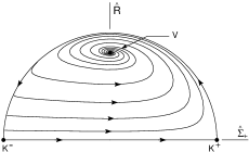
Figure 3: Orbits in the invariant set $S_{\hat{\Omega}}$.

We now consider the case $\frac{4}{3}<\gamma\leqslant 2$. The flow on the invariant set $S_{\hat{\Omega}}$ is depicted in figure 3, which shows the projection of the surface $\hat{\Omega}=0$ onto the $\hat{\Sigma}_{+}\hat{R}$-plane. The essential features are the existence of three equilibrium points

$$\mathsf{K}^{\pm}: \quad(\hat{\Sigma}_{+},\hat{R},\hat{\mathcal{H}})=(\pm 1,0,0),$$

$$\mathsf{V}: \quad(\hat{\Sigma}_{+},\hat{R},\hat{\mathcal{H}})=\left(0,\sqrt{{\textstyle\frac{2}{3}}},\sqrt{2}\right),$$

in which $\mathsf{K}^{\pm}$ lie on the boundary of $S_{\hat{\Omega}}$, and the fact that there are no periodic orbits on $S_{\hat{\Omega}}$. The latter can be established by the existence of a Dulac function $\lambda$ on $S_{\hat{\Omega}}$ given by

$$\lambda=\hat{R}^{-3}(1-\hat{\Sigma}_{+}^{2}-\hat{R}^{2})^{-2}$$

(see [19], theorem 4.6, pg. 94). Thus, the only potential $\omega$-limit sets in $S_{\hat{\Omega}}$ are the equilibrium points $\mathsf{K}^{\pm}$, $\mathsf{V}$ and the heteroclinic sequence $(\mathsf{K}^{-}\rightarrow\mathsf{K}^{+}\rightarrow\mathsf{K}^{-})$ and hence for any $\hat{\boldsymbol{x}}\in S_{\hat{\Omega}}$, the $\omega$-limit set is one of these four candidates. The point $\mathsf{K}^{+}$ can be excluded since it is a local source in $S$. Moreover, the point $\mathsf{K}^{-}$ can be excluded by considering the evolution equation for $\hat{\mathcal{H}}$, which is of the form

$$\hat{\mathcal{H}}^{\prime}=h(\hat{\Sigma}_{+},\hat{R},\hat{\mathcal{H}})\hat{\mathcal{H}}.$$

Since $h(\mathsf{K}^{-})=h(-1,0,0)=3$ and $\hat{\mathcal{H}}=0$ at $\mathsf{K}^{-}$, it follows that $\lim_{\tau\rightarrow+\infty}\hat{\mathcal{H}}\not=0$ and hence that an orbit in $S$ cannot be future asymptotic to $\mathsf{K}^{-}$. This leaves the equilibrium point $\mathsf{V}$ and the heteroclinic sequence $(\mathsf{K}^{-}\rightarrow\mathsf{K}^{+}\rightarrow\mathsf{K}^{-})$ as the remaining candidates for the $\omega$-limit set in $S_{\hat{\Omega}}$. The latter can be excluded since $\mathsf{V}$ is a local sink in $S$ and hence $\omega(\hat{\boldsymbol{x}})=\mathsf{V}$ for any $\hat{x}\in S_{\hat{\Omega}}$. On account of (B.11), we thus conclude that for any $\hat{\boldsymbol{x}}\in S$,

$$\lim_{\tau\rightarrow+\infty}(\hat{\Sigma}_{+},\hat{R},\hat{\mathcal{H}})=\left(0,\sqrt{{\textstyle\frac{2}{3}}},\sqrt{2}\right),\qquad\text{if}\quad{\textstyle\frac{4}{3}}<\gamma\leqslant 2$$ (B.12)

The case $\frac{2}{3}<\gamma<\frac{4}{3}$ can be treated in a similar fashion by analyzing the dynamics on the invariant sets $S_{\hat{R}}$ and $S_{\hat{\mathcal{H}}}$. It follows that

$$\lim_{\tau\rightarrow+\infty}(\hat{\Sigma}_{+},\hat{R},\hat{\mathcal{H}})=(0,0,0),\qquad\text{if}\quad{\textstyle\frac{2}{3}}<\gamma\leqslant{\textstyle\frac{4}{3}}.$$ (B.13)

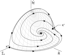
Figure 4: Orbits in the invariant set $\hat{\Omega}^{3}/(\hat{R}^{4}\hat{\mathcal{H}}^{2})=k$ with $k>0$ and $\gamma=\frac{4}{3}$.

Finally, we consider the case $\gamma=\frac{4}{3}$. We first observe that the $\hat{\Omega}$ evolution equation (B.6) restricted to a radiation fluid reduces to

$$\hat{\Omega}^{\prime}=2\hat{\Sigma}_{+}^{2}\hat{\Omega}.$$

It follows immediately from the LaSalle invariance principle (see [19], theorem 4.11, pg. 103) that

$$\omega(\hat{\boldsymbol{x}})\subset\{\hat{\boldsymbol{x}}\>|\>\Sigma_{+}=0\},$$ (B.14)

for any $\hat{\boldsymbol{x}}\in S$. By (B.9) the function $Z$ defined in (B.8) describes a conserved quantity

$$\frac{\hat{\Omega}^{3}}{\hat{R}^{4}\hat{\mathcal{H}}^{2}}=k,$$ (B.15)

where $k>0$ is a constant that depends on the initial condition. We see that for all $k>0$ the surfaces described by (B.15) foliate the state space $S$ and intersect the boundary $\hat{\Omega}=0$ at $\hat{R}=0$ and $\hat{\mathcal{H}}=0$ (see figure 4). When $\gamma=\frac{4}{3}$, the DE (B.3) has a line $\mathsf{L}$ of equilibrium points given by

$$\mathsf{L}:\quad(\hat{\Sigma}_{+},\hat{R},\hat{\mathcal{H}})=\left(0,\sqrt{{\textstyle\frac{2}{3}}}\,k,\sqrt{2}\,k\right),\quad k\in(0,1).$$

It can show that for each $k>0$, the two-dimensional invariant set defined by (B.15) intersects the line $\mathsf{L}$ at precisely one point. Since this unique point of intersection is the only equilibrium point on this invariant set which satisfies $\hat{\Sigma}_{+}=0$, it follows from the restriction (B.14) that any solution in $S$ satisfies

$$\lim_{\tau\rightarrow+\infty}(\hat{\Sigma}_{+},\hat{R},\hat{\mathcal{H}})=\left(0,\sqrt{{\textstyle\frac{2}{3}}}\,k,\sqrt{2}\,k\right),\qquad\text{if}\quad\gamma={\textstyle\frac{4}{3}},$$ (B.16)

where $k\in(0,1)$ is a constant which depends on the initial condition.

Appendix B.2

We now apply theorem B.1 using the results of appendix B.1 to prove that

$$\lim_{\tau\rightarrow+\infty}\bar{\boldsymbol{x}}=\boldsymbol{a},$$

where $\bar{\boldsymbol{x}}=(\bar{\Sigma}_{+},\bar{R},\bar{\mathcal{H}})$ and $\boldsymbol{a}$ is given by the right-hand sides of (B.12), (B.13) and (B.16), considering the three cases $\frac{2}{3}<\gamma<\frac{4}{3}$, $\gamma=\frac{4}{3}$ and $\frac{4}{3}<\gamma\leqslant 2$ simultaneously.

We begin by defining the subset $D$ in theorem B.1 by

$$\Sigma_{+}^{2}+R^{2}+{\textstyle\frac{1}{6}}\mathcal{H}^{2}<1.$$

We now verify the hypotheses $H_{1}$ and $H_{2}$. Firstly, let $\boldsymbol{w}:[\tau_{0},+\infty)\rightarrow D$ be any $C^{0}[\tau_{0},\infty)$ function. Since $\lim_{\tau\rightarrow+\infty}M(\tau)=0$ it follows immediately from (3.12) that

$$\lim_{\tau\rightarrow+\infty}\boldsymbol{g}(\boldsymbol{w}(\tau),\tau)=\lim_{\tau\rightarrow+\infty}M(\tau)\left(B_{\bar{\Sigma}_{+}},\bar{R}B_{\bar{R}},\bar{\mathcal{H}}B_{\bar{\mathcal{H}}}\right)\Big{|}_{\bar{\boldsymbol{x}}=\boldsymbol{w}(\tau)}=\mathbf{0},$$

showing that $H_{1}$ is satisfied. Secondly, $H_{2}$ is satisfied since the variables $\bar{\Sigma}_{+}$, $\bar{R}$ and $\bar{\mathcal{H}}$ are bounded for all $\tau\geqslant\tau_{0}$ with $\tau_{0}$ sufficiently large. Therefore, since

$$\lim_{\tau\rightarrow+\infty}\hat{\boldsymbol{x}}(\tau)=\boldsymbol{a}$$

for all initial conditions $\hat{\boldsymbol{x}}(\tau_{0})$ in $D$ (see (B.12), (B.13) or (B.16)), theorem B.1 implies that

$$\lim_{\tau\rightarrow+\infty}\bar{\boldsymbol{x}}(\tau)=\boldsymbol{a}$$ (B.17)

for all initial conditions $\bar{\boldsymbol{x}}(\tau_{0})$ in $D$.

Finally, we need to show that any initial condition $\boldsymbol{x}(\tau_{0})=(\Sigma_{+},R,\mathcal{H})\big{|}_{\tau=\tau_{0}}$, $M(\tau_{0})$, $\psi(\tau_{0})$ for the DE (2.21), subject to $\Omega>0$ and (2.25), determines an initial condition $\bar{\boldsymbol{x}}(\tau_{0})$ in $D$ for the DE (3.11), so that (B.17) is satisfied. Indeed, since $\lim_{\tau\rightarrow+\infty}\psi=+\infty$, we can without loss of generality restrict the initial condition $\psi(\tau_{0})$ to be a multiple of $\pi$. This requirement can be achieved by simply following the solution determined by the original initial condition until this condition is satisfied. It follows from this condition, in conjunction with (3.8) and the restriction $\Omega>0$ applied to (2.23), that

$$\left.\left(\bar{\Sigma}_{+}^{2}+\bar{R}^{2}+{\textstyle\frac{1}{6}}\bar{\mathcal{H}}^{2}\right)\right|_{\tau=\tau_{0}}=\left.\left(\Sigma_{+}^{2}+R^{2}+{\textstyle\frac{1}{6}}\mathcal{H}^{2}\right)\right|_{\tau=\tau_{0}}<1,$$

so that $\bar{\boldsymbol{x}}(\tau_{0})\in D$.

Appendix B.3

We now provide the proof of (3.5) for the case $\frac{2}{3}<\gamma<\frac{4}{3}$, which gives the limit of the ratio $R/M$ at late times. In analogy to (3.8), we define a variable $\bar{M}$ by

$$\bar{M}=M\left(1+{\textstyle\frac{1}{4}}R^{2}M\sin 2\psi\right).$$ (B.18)

It follows from (2.21) that the evolution equation for $\bar{M}$ is of the form

$$\bar{M}^{\prime}=-(\bar{Q}+2\bar{\Sigma}_{+}+MB_{\bar{M}})\bar{M},$$ (B.19)

where $B_{\bar{M}}$ is a bounded function for $\tau$ sufficiently large. By using (3.9) we obtain

$$\left(\frac{\bar{R}}{\bar{M}}\right)^{\prime}=\left[3(\gamma-1)+h(\bar{\boldsymbol{x}},M,\psi)\right]\left(\frac{\bar{R}}{\bar{M}}\right),$$ (B.20)

where

$$h(\bar{\boldsymbol{x}},M,\psi)=2-3\gamma+2\bar{Q}+3\bar{\Sigma}_{+}+MB_{*}$$

and $B_{\ast}$ is a bounded function for $\tau$ sufficiently large. It follows from (3.6), (3.8), (3.10) and theorem 3.5 that $\lim_{\tau\rightarrow+\infty}h(\bar{\boldsymbol{x}},M,\psi)=0$. Consequently, (B.20) implies that

$$\frac{\bar{R}}{\bar{M}} =\mathcal{O}\left(\mathrm{e}^{[3(\gamma-1)+\delta]\tau}\right),\qquad\text{if}\quad{\textstyle\frac{2}{3}}\leqslant\gamma<1,$$

$$\frac{\bar{M}}{\bar{R}} =\mathcal{O}\left(\mathrm{e}^{[3(1-\gamma)+\delta]\tau}\right),\qquad\text{if}\quad 1<\gamma<{\textstyle\frac{4}{3}},$$

as $\tau\rightarrow+\infty$ for any $\delta>0$. Therefore, on account of (B.18) and (3.8),

$$\lim_{\tau\rightarrow+\infty}\frac{R}{M}=\begin{cases}0,&\text{if}\quad\frac{2}{3}\leqslant\gamma<1,\\ +\infty,&\text{if}\quad 1<\gamma<\frac{4}{3}.\end{cases}$$

It remains to deduce the limit of $R/M$ as $\tau\rightarrow+\infty$ for the case $\gamma=1$. To proceed we compute the asymptotic form of $R$ and $M$ as $\tau\rightarrow+\infty$. The calculation parallels that for the non-magnetic Bianchi VII₀ models detailed in appendix B of [20]. It follows that any solution of the DE (2.21) subject to the restrictions (2.25) with $\frac{2}{3}<\gamma<\frac{4}{3}$ satisfies

$$\Sigma_{+} =\frac{2(C_{\mathcal{H}}^{2}-3C_{R}^{2})}{3(3\gamma-2)}\,\mathrm{e}^{(3\gamma-4)\tau}\left[1+\mathcal{O}(\mathrm{e}^{-b\tau})\right],$$

$$R =C_{R}\,\mathrm{e}^{1/2\,(3\gamma-4)\tau}\left[1+\mathcal{O}(\mathrm{e}^{-b\tau})\right],$$

$$\mathcal{H} =C_{\mathcal{H}}\,\mathrm{e}^{1/2\,(3\gamma-4)\tau}\left[1+\mathcal{O}(\mathrm{e}^{-b\tau})\right],$$

$$M =C_{M}\,\mathrm{e}^{1/2\,(2-3\gamma)\tau}\left[1+\mathcal{O}(\mathrm{e}^{-b\tau})\right],$$

as $\tau\rightarrow+\infty$, for some constant $b>0$, where $C_{R}$, $C_{\mathcal{H}}$ and $C_{M}$ are positive constants which depend on the initial conditions. Therefore,

$$\frac{R}{M}=\frac{C_{R}}{C_{M}}\,\mathrm{e}^{3(\gamma-1)\tau}\left[1+\mathcal{O}(\mathrm{e}^{-b\tau})\right]$$

as $\tau\rightarrow+\infty$ and hence

$$\lim_{\tau\rightarrow+\infty}\frac{R}{M}=\frac{C_{R}}{C_{M}}\not=0,\qquad\text{if}\quad\gamma=1.$$

Appendix C

In this appendix we give an expression for the Weyl curvature parameter $\mathcal{W}$ in terms of the Hubble-normalized variables $\Sigma_{+}$, $R$, $\mathcal{H}$, $M$ and $\psi$. Let $E_{\alpha\beta}$ and $H_{\alpha\beta}$ be the components of the electric and magnetic parts of the Weyl tensor relative to the group invariant frame with $\boldsymbol{e}_{0}=\boldsymbol{u}$. It follows that $E_{\alpha\beta}$ and $H_{\alpha\beta}$ are diagonal and trace-free and hence they each have two independent components. In analogy with (2.3) we define

$$\begin{split}\mathcal{E}_{+}={\textstyle\frac{1}{2}}(\mathcal{E}_{22}+\mathcal{E}_{33}),&\qquad\mathcal{E}_{-}={\textstyle\frac{1}{2\sqrt{3}}}(\mathcal{E}_{22}-\mathcal{E}_{33}),\\ \mathcal{H}_{+}={\textstyle\frac{1}{2}}(\mathcal{H}_{22}+\mathcal{H}_{33}),&\qquad\mathcal{H}_{-}={\textstyle\frac{1}{2\sqrt{3}}}(\mathcal{H}_{22}-\mathcal{H}_{33}),\end{split}$$ (C.1)

where $\mathcal{E}_{\alpha\beta}$ and $\mathcal{H}_{\alpha\beta}$ are the dimensionless counterparts of $E_{\alpha\beta}$ and $H_{\alpha\beta}$, defined by

$$\mathcal{E}_{\alpha\beta}=\frac{E_{\alpha\beta}}{H^{2}},\qquad\mathcal{H}_{\alpha\beta}=\frac{H_{\alpha\beta}}{H^{2}}.$$ (C.2)

It follows from (3.2), (C.1) and (C.2) that

$$\mathcal{W}^{2}=\mathcal{E}_{+}^{2}+\mathcal{E}_{-}^{2}+\mathcal{H}_{+}^{2}+\mathcal{H}_{-}^{2}.$$ (C.3)

Equations (1.101) and (1.102) in [19] for $E_{\alpha\beta}$ and $H_{\alpha\beta}$, in conjunction with the frame choice detailed in section 2 of [8] and equations (C.1) and (2.20) in the present paper lead to

$$\begin{split}\mathcal{E}_{+}&=\Sigma_{+}(1+\Sigma_{+})+{\textstyle\frac{1}{2}}R^{2}(1-3\cos 2\psi)-{\textstyle\frac{1}{6}}\mathcal{H}^{2},\\ \mathcal{H}_{+}&=-{\textstyle\frac{3}{2}}R^{2}\sin 2\psi,\\ \mathcal{E}_{-}&=\frac{2R}{M}\left[\sin\psi+{\textstyle\frac{1}{2}}M(1-2\Sigma_{+})\cos\psi\right],\\ \mathcal{H}_{-}&=\frac{2R}{M}\left[-\cos\psi-{\textstyle\frac{3}{2}}M\Sigma_{+}\sin\psi\right].\end{split}$$ (C.4)

References

- [1] Barrow, J., Ferreira, P. G., and Silk, J. (1997). Constraints on a Primordial Magnetic Field. Phys. Rev. Lett. 78, 3610–3.
- [2] Collins, C. B. (1972). Qualitative Magnetic Cosmology. Commun. Math. Phys. 27, 37–43.
- [3] Crowe, S. R. (1998). Dynamical Systems Analysis of Magnetic Bianchi III Cosmologies. MMath Thesis, University of Waterloo, unpublished.
- [4] Ellis, G. F. R., and MacCallum, M. A. H. (1969). A Class of Homogeneous Cosmological Models. Commun. Math. Phys. 12, 108–41.
- [5] Horwood, J. T., Hancock, M. J., The, D., and Wainwright, J. (2003). Late-Time Asymptotic Dynamics of Bianchi VIII Cosmologies. Class. Quantum Grav. 20, 1757–78.
- [6] LeBlanc, V. G. (1997). Asymptotic States of Magnetic Bianchi I Cosmologies. Class. Quantum Grav. 14, 2281–301.
- [7] LeBlanc, V. G. (1998). Bianchi II Magnetic Cosmologies. Class. Quantum Grav. 18, 1607–26.
- [8] LeBlanc, V. G., Kerr, D., and Wainwright, J. (1995). Asymptotic States of Magnetic Bianchi VI0 Cosmologies. Class. Quantum Grav. 12, 513–41.
- [9] Maartens, R., Ellis, G. F. R., and Stoeger, W. R. (1996). Anisotropy and inhomogeneity of the universe from . Astron. Astrophys. 309, L7–L10.
- [10] Maartens, R., Tsagas, C. G., and Ungarelli, C. (2001). Magnetized Gravitational Waves. Phys. Rev. D. 63, 123507.
- [11] Matravers, D. R, and Tsagas, C. G. (2000). Cosmic Magnetism, Curvature and the Expansion Dynamics. Phys. Rev. D. 62, 103519.
- [12] Strauss, A., and Yorke, J. A. (1967). On Asymptotically Autonomous Differential Equations. Math. Syst. Theory. 1, 175–82.
- [13] Tsagas, C. G. (2001). Magnetic Tension and the Geometry of the Universe. Phys. Rev. Lett. 86, 5421–4.
- [14] Tsagas, C. G., and Barrow, J. D. (1997). A Gauge-Invariant Analysis of Magnetic Fields in General-Relativistic Cosmology. Class. Quantum Grav. 14, 2539–62.
- [15] Tsagas, C. G., and Barrow, J. D. (1998). Gauge-Invariant Magnetic Perturbations in Perfect-Fluid Cosmologies. Class. Quantum Grav. 15, 3523–44.
- [16] Tsagas, C. G., and Maartens, R. (2000). Cosmological Perturbations on a Magnetized Bianchi I Background. Class. Quantum Grav. 17, 2215–41.
- [17] Tsagas, C. G., and Maartens, R. (2000). Magnetized Cosmological Perturbations. Phys. Rev. D. 61, 083519.
- [18] Uggla, C., van Elst, H., Wainwright, J., and Ellis, G. F. R. (2003). The Past Attractor in Inhomogeneous Cosmology. Preprint gr-qc/0304002. (to appear in Phys. Rev. D).
- [19] Wainwright, J., and Ellis, G. F. R, eds. (1997). Dynamical Systems in Cosmology (Cambridge University Press).
- [20] Wainwright, J., Hancock, M. J., and Uggla, C. (1999). Asymptotic Self-Similarity Breaking at Late Times in Cosmology. Class. Quantum Grav. 16, 2577–98.
- [21] Weaver, M., Isenberg, J., and Berger, B. K. (1998). Mixmaster Behavior in Inhomogeneous Cosmological Spacetimes. Phys. Rev. Lett. 80, 2984–7.