Gravitating Fermionic Lumps with a False Vacuum Core

Abstract

We investigate gravitating lumps with a false vacuum core surrounded by the true vacuum in a scalar field potential. Such configurations become possible in Einstein gravity in the presence of fermions at the core. Gravitational interactions as well as Yukawa interactions are essential for such lumps to exist. The mass and size of gravitating lumps sensitively depend on the scale characterizing the scalar field potential and the density of fermions. These objects can exist in the universe at various scales.

1 Introduction

When a scalar field potential has two non-degenerate minima, the absolute minimum of the potential corresponds to the true vacuum, while the other to the false vacuum. Systems in which false and true vacua coexist are of great interest. The universe is full of various structures such as black holes, stars and dark matter. Does there exist any structure that has a false vacuum in its core? If the entire universe is in a false vacuum, it decays into the true vacuum through bubble creation by quantum tunneling.[1] What happens if a false vacuum core is surrounded by the true vacuum?[2, 3] If the size of the core is smaller than the critical radius, the core would quickly decay, with its energy dissipating to the spatial infinity. If the size of the core is larger than the critical radius, the core becomes a black hole. In either case the configuration cannot be static. The fate of false-vacuum bubbles has been extensively discussed in the literature.[4, 5, 6]

It has been shown recently that new configurations, cosmic shells, emerge in a simple real scalar field theory in which spherical shells of the true vacuum are immersed in the false vacuum.[7] Such static cosmic shells can exist thanks to gravitational interactions. However, a static ball of the false vacuum immersed in the true vacuum is not possible.

In this paper we demonstrate that a static false vacuum core becomes possible if there is additional matter coupled to the scalar field such as fermions. The number of fermions necessary is not large. Gravitational interactions as well as Yukawa interactions play a key role in making such a structure possible. It is a gravitating fermionic lump. We stress that gravitating lumps are quite different from Q-balls, boson stars and Fermi-balls. In Q-balls the conserved charge of the scalar field plays a central role in realizing the stability.[8] There is no such charge of the scalar field in our model. In boson stars, gravitational interactions as well as the conserved charge play a key role.[9, 10] The model for Fermi balls is very similar to ours [11, 12] in which the false vacuum is surrounded by the true vacuum. In Fermi balls, fermions are localized in the transition region, or the domain wall, i.e. they reside in the surface region of the lumps. In our model fermions reside in the bulk region inside the lump and the Yukawa interaction becomes essential.

Gravitational interactions can produce lump solutions in non-Abelian gauge theory as well. Even in the pure Einstein-Yang-Mills theory stable monopole solutions appear in the asymptotically anti-de Sitter space.[13, 14, 15] We show in the present paper that such gravitational lumps appear even in a simple scalar field theory with fermions.

The spacetime geometry of gravitating lumps is either anti-de Sitter-Schwarzschild or de Sitter-Schwarzschild. Dymnikova has discussed the global structure of de Sitter-Schwarzschild spacetime, assuming an appropriate external matter distribution.[16] The existence of gravitating lumps in the present paper shows that anti-de Sitter-Schwarzschild spacetime is indeed realized in a very simple system. Its existence can be inferred from the energetics consideration in flat spacetime as well. The extension to de Sitter-Schwarzschild spacetime is reserved for future investigation. One may explore such objects in the universe at various scales and epochs. We shall see that the size of gravitating lumps sensitively depends on the scale characterizing the scalar field potential.

We stress that the gravitating fermionic lumps described in the present paper exist when there appears a false vacuum and there are fermions coupled to the relevant scalar field. Recently it has been shown that such a false vacuum appears in the early universe in the standard Einstein-Weinberg-Salam theory of electroweak and gravitational interactions, if the universe has a spatial section $S^{3}$ as in the closed Friedmann-Robertson-Walker universe.[17] In the early stage, nontrivial gauge fields yield a false vacuum in the Higgs field, to which quarks and leptons have Yukawa couplings. In other words gravitating fermionic lumps may be copiously produced in the framework of the standard model.

In §2 we set up the problem and introduce useful variables in terms of which the field equations are written. In §3 we give the energetics of fermionic lumps, based mainly on flat spacetime. This illustrates how such lumps become possible when the scalar field potential has a false vacuum configuration. In §4 the behavior of the solutions is investigated analytically inside the lump, numerically in the transition region, and analytically outside the lump. More details of the solutions are given in §5 with a focus on the dependence of the solutions on various parameters of the model. It is seen how the solutions change as the energy scale of the model is lowered. A summary and conclusions are given in §6.

2 Model

We consider a real scalar field in the Einstein gravity whose Lagrangian is given by

$$\mathcal{L}=\frac{1}{16\pi G}R+\frac{1}{2}g^{\mu\nu}\partial_{\mu}\phi\partial_{\nu}\phi-V[\phi]-\phi\rho_{S}(x)$$ (1)

where $R$ and $V[\phi]$ are the scalar curvature and the scalar potential, respectively. The last term in (1) represents a source for the scalar field. It naturally arises if there is a fermion field $\psi$ with a Yukawa interaction $-g\phi\bar{\psi}\psi$.[18] In this case $\rho_{S}(x)=g\raise 0.68889pt\hbox{$\langle$}\lower 0.68889pt\hbox{}\psi\kern-6.49994pt\raise 6.00006pt\hbox{$-$}\lower 6.00006pt\hbox{}\psi\,\raise 0.68889pt\hbox{$\rangle$}\lower 0.68889pt\hbox{}$. As shown schematically in Fig. 1, $V[\phi]$ has two minima at $f_{1}$ and $f_{2}$. We take

$$V[\phi]\, = \frac{\lambda}{4}(\phi-f_{2})\Bigg{\{}\phi^{3}-\frac{1}{3}(f_{2}+4f_{1})\phi^{2}-\frac{1}{3}f_{2}(f_{2}-2f_{1})(\phi+f_{2})\Bigg{\}}~{},$$ (2)

$$V^{\prime}[\phi] = \lambda\phi(\phi-f_{1})(\phi-f_{2})~{}.$$ (3)

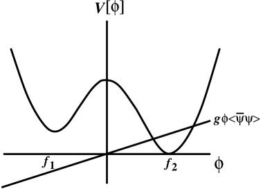
Figure 1: A scalar field potential $V[\phi]$ with two minima. The quantity $\phi\rho_{S}=g\phi\raise 0.68889pt\hbox{$\langle$}\lower 0.68889pt\hbox{}\psi\kern-6.49994pt\raise 6.00006pt\hbox{$-$}\psi\,\raise 0.68889pt\hbox{$\rangle$}\lower 0.68889pt\hbox{}$ at the core is also displayed for $g\raise 0.68889pt\hbox{$\langle$}\lower 0.68889pt\hbox{}\psi\kern-6.49994pt\raise 6.00006pt\hbox{$-$}\psi\,\raise 0.68889pt\hbox{$\rangle$}\lower 0.68889pt\hbox{}>0$. In the lump solutions described in the present paper, $g|f_{1}|\raise 0.68889pt\hbox{$\langle$}\lower 0.68889pt\hbox{}\psi\kern-6.49994pt\raise 6.00006pt\hbox{$-$}\psi\,\raise 0.68889pt\hbox{$\rangle$}\lower 0.68889pt\hbox{}$ is much larger than the energy density of the false vacuum at $f_{1}$.

In the potential $V[\phi]$, the false vacuum appears at $\phi=f_{1}$ and the true vacuum at $\phi=f_{2}$. We investigate spherically symmetric configurations in which the scalar field varies from the false vacuum to the true vacuum as the radius $r$ increases. Solutions $\phi(r)$ are to satisfy the two conditions (i) $\phi(0)\simeq f_{1}$ and (ii) $\phi(\infty)=f_{2}$.

In (1) we have added the interaction term $-\phi\rho_{S}(x)$ to the scalar field. This interaction is vital to have solutions satisfying the condition (ii). As we shall see below, solutions regular at the origin are uniquely specified by the value of $\phi(0)$ with a given $\rho_{S}(x)$. Without the coupling to a source $-\phi\rho_{S}(x)$, the configuration $\phi(r)$ either settles at $\phi=0$ after oscillation as $r\rightarrow\infty$, which corresponds to a totally unstable configuration, or comes back to $\phi=f_{1}$, or overshoots $\phi=f_{1}$ to diverge to $-\infty$ as $r$ approaches $\infty$. Solutions of the second type indeed exist. They are cosmic shells.[7] The source term $-\phi\rho_{S}(x)$ gives a $x$-dependent linear potential for the scalar field. (See Fig. 1.)

We treat the system classically. If the source comprises fermions, $\rho_{S}(x)=g\raise 0.68889pt\hbox{$\langle$}\lower 0.68889pt\hbox{}\psi\kern-6.49994pt\raise 6.00006pt\hbox{$-$}\lower 6.00006pt\hbox{}\psi(x)\,\raise 0.68889pt\hbox{$\rangle$}\lower 0.68889pt\hbox{}$ where $g$ is a Yukawa coupling constant. If the fermions at the core are nonrelativistic, $\raise 0.68889pt\hbox{$\langle$}\lower 0.68889pt\hbox{}\psi\kern-6.49994pt\raise 6.00006pt\hbox{$-$}\lower 6.00006pt\hbox{}\psi(x)\,\raise 0.68889pt\hbox{$\rangle$}\lower 0.68889pt\hbox{}$ can be approximated by the fermion density $\raise 0.68889pt\hbox{$\langle$}\lower 0.68889pt\hbox{}\psi^{\dagger}\psi(x)\,\raise 0.68889pt\hbox{$\rangle$}\lower 0.68889pt\hbox{}\equiv\rho_{n}(x)$. In the present paper we suppose that the fermion density is small enough so that the back-reaction to the metric can be ignored. This condition is met in a simple model if the fermion couples to a pair of scalar fields in the specific manner described in the next section. A full treatment of the dynamics of the sources including back-reaction to the Einstein equations is left for a future study.

We look for spherically symmetric, static configurations. The metric of spacetime is written as

$$ds^{2}=\frac{H}{p^{2}}dt^{2}-\frac{dr^{2}}{H}-r^{2}(d\theta^{2}+\sin^{2}\theta d\varphi^{2})$$ (4)

where $H$ and $p$ are functions depending only on $r$. In the tetrad basis

$$e_{0}=\frac{\sqrt{H}}{p}dt~{},~{}~{}e_{1}=\frac{1}{\sqrt{H}}dr~{},~{}~{}e_{2}=rd\theta~{},~{}~{}e_{3}=r\sin\theta d\varphi~{},$$ (5)

the energy-momentum tensors $T_{ab}=e_{a}^{\ \mu}e_{b}^{\ \nu}T_{\mu\nu}$ are

$$\hskip-28.45274ptT_{00}=\frac{1}{2}H{\phi^{\prime}}^{2}+V[\phi]+\phi\rho_{S}~{},$$ (6)

$$\hskip-28.45274ptT_{11}=\frac{1}{2}H{\phi^{\prime}}^{2}-V[\phi]-\phi\rho_{S}~{},$$ (7)

$$\hskip-28.45274ptT_{22}=T_{33}=-\frac{1}{2}H{\phi^{\prime}}^{2}-V[\phi]-\phi\rho_{S}~{},$$ (8)

$$\hskip-28.45274pt\hbox{others}=0~{}~{},$$ (9)

where the prime represents a $r$-derivative.

The Einstein equations are

$$-\frac{H^{\prime}}{r}+\frac{1-H}{r^{2}} = 8\pi G\,T_{00}~{},$$ (10)

$$\frac{1}{r}\Bigl{(}-\frac{2Hp^{\prime}}{p}+H^{\prime}\Bigr{)}-\frac{1-H}{r^{2}} = 8\pi G\,T_{11}~{},$$ (11)

$$\frac{p}{2}\frac{\partial}{\partial r}\Bigl{(}\frac{H^{\prime}}{p}-\frac{2Hp^{\prime}}{p^{2}}\Bigr{)}-\frac{Hp^{\prime}}{rp}+\frac{H^{\prime}}{r} = 8\pi G\,T_{22}~{}.$$ (12)

It follows from (10) that

$$H=1-\frac{2GM}{r}~{}~{},~{}~{}M=\int_{0}^{r}4\pi r^{2}dr\,T_{00}~{}~{}.$$ (13)

Adding (10) to (11), we find

$$\frac{p^{\prime}}{p}=-4\pi Gr{\phi^{\prime}}^{2}~{}~{}.$$ (14)

$p(r)$ is a monotonically decreasing function. The equation of motion for the scalar field is

$$-\frac{p}{r^{2}}\frac{\partial}{\partial r}\Bigl{(}\frac{r^{2}H}{p}\phi^{\prime}\Bigr{)}+V^{\prime}[\phi]+\rho_{S}=0.$$ (15)

Eq. (12) follows from Eqs. (10), (11), and (15).

After eliminating $p(r)$, the equations are reduced to (13) and

$$\phi^{\prime\prime}(r)+\bigg{(}\frac{2}{r}+4\pi Gr{\phi^{\prime}(r)}^{2}+\frac{H^{\prime}}{H}\bigg{)}\phi^{\prime}(r)=\frac{1}{H}\Big{(}V^{\prime}[\phi]+\rho_{S}\Big{)}~{}~{}.$$ (16)

In interpreting Eq. (16) it is convenient to introduce the new coordinate $\xi$ as

$$\xi(r)=\int_{0}^{r}{dr\over\sqrt{H}}~{}~{}.$$ (17)

In the examples discussed below $H(r)$ remains positive definite so that $\xi(r)$ is well defined. Then the equation reads

$$\hskip-28.45274pt{d^{2}\phi\over d\xi^{2}}+\Gamma(\xi){d\phi\over d\xi}=V^{\prime}[\phi]+\rho_{S}(\xi)~{}~{},$$ (18)

$$\hskip-28.45274pt\Gamma(\xi)=\sqrt{H}\bigg{(}\frac{2}{r}+4\pi Gr{\phi^{\prime}(r)}^{2}+\frac{H^{\prime}}{2H}\bigg{)}~{}~{}.$$ (19)

In terms of the “time” coordinate $\xi$ a particle with position $\phi(\xi)$ moves in the potential $-V[\phi]$ with a time-dependent external force $\rho_{S}(\xi)$. There is friction $\Gamma$ which can be either positive or negative. The solution we are looking for corresponds to a particle which starts from $\sim f_{1}$ and moves to $f_{2}$ asymptotically. It must gain an energy as $-V[f_{1}]<-V[f_{2}]$, which is possible as there is an additional force given by $\rho_{S}$ and $\Gamma$ can be negative.

Equations (13) and (16) define a set of nonlinear equations. To be definite we suppose that the source to $\phi$ is given by

$$\rho_{S}(r)=\rho_{0}\theta(R_{1}-r)~{}~{}.$$ (20)

We split the space into three regions:

$${\rm I.}\quad 0\leq r\leq R_{1}$$ (21)

$${\rm II.}\quad R_{1}\leq r\leq R_{2}$$ (22)

$${\rm III.}\quad R_{2}\leq r<\infty$$

In region I, the spacetime is approximately anti-de Sitter with $\rho_{S}>0$ and $\phi_{0}$ very close to, but still greater than, the location $f_{S}$ of the minimum of $V[\phi]+\phi\rho_{S}$: $\phi(0)=f_{S}+\delta\phi(0)$ with $0<\delta\phi(0)/|f_{S}|\ll 1$. It turns out that $\phi(r)$ varies little from $f_{S}$ in region I so that the equation of motion for $\phi$ may be linearized in this region. In region II, $\rho_{S}=0$. In this region the field varies significantly so that the full set of nonlinear equations must be solved numerically. In region III, $\rho_{S}=0$ and the spacetime is approximately Schwarzschild. In this paper we focus on the case in which $|f_{1}|\sim f_{2}\sim f\equiv\hbox{${1\over 2}$}(|f_{1}|+f_{2})$, $f_{r}=(f_{2}-|f_{1}|)/f\ll 1$ and $|f_{1}-f_{S}|\ll f$ so that the linearization of Eq. (16) is valid. The behavior of a solution $\phi(r)$ is displayed schematically in Fig.  2.

Figure 2: The behavior of $\phi(r)$. In the lump solutions $|f_{1}-f_{S}|\ll|f_{1}|$ and $R_{2}-R_{1}\ll R_{1}$.

Figure 3: The behavior of $H(r)$. $H^{\prime}(r)$ is discontinuous at $R_{1}$ as $T_{00}$ is discontinuous there when $\rho_{S}$ is given by (20).

Figure 4: The behavior of $p(r)$.

3 Energetics of fermionic lumps

It is instructive to see how fermionic lumps become possible from consideration of energetics in flat spacetime. The basic idea is that there reside nonrelativistic fermions at the core, which generate an additional linear interaction $\phi\rho_{S}$. For nonrelativistic fermions $\raise 0.68889pt\hbox{$\langle$}\lower 0.68889pt\hbox{}\psi\kern-6.49994pt\raise 6.00006pt\hbox{$-$}\lower 6.00006pt\hbox{}\psi\,\raise 0.68889pt\hbox{$\rangle$}\lower 0.68889pt\hbox{}\sim\raise 0.68889pt\hbox{$\langle$}\lower 0.68889pt\hbox{}\psi^{\dagger}\psi\,\raise 0.68889pt\hbox{$\rangle$}\lower 0.68889pt\hbox{}\equiv\rho_{n}$ so that the Yukawa interaction $g\phi\psi\kern-6.49994pt\raise 6.00006pt\hbox{$-$}\lower 6.00006pt\hbox{}\psi$ generates a linear potential $g\rho_{n}\phi$ for the scalar field inside the lump. Let $R$ be the radius of the lump. We suppose that the total fermion number $N_{F}$ is conserved. $N_{F}$ is kept fixed in the consideration below.

The scalar potential $V[\phi]$ takes the form depicted in Fig. 1. The total potential $V[\phi]+g\rho_{n}\phi$ has a minimum at $f_{S}<0$. It is supposed that $V[f_{1}]\equiv\epsilon_{0}>0$ but the energy density at the minimum $V[f_{S}]+g\rho_{n}f_{S}=\epsilon<0$ becomes negative for the lump solution. $f_{S}$ and $\epsilon$ depends on $\rho_{n}$ or equivalently on $R$.

Inside the lump $r<R$, the scalar field satisfies $\phi\sim f_{S}$ whereas outside the lump $\phi=f_{2}$. A degenerate nonrelativistic fermion gas has energy density ${\cal E}_{f}=mc^{2}\rho_{n}+A\rho_{n}^{5/3}$ where $A=3(3\pi^{2})^{2/3}\hbar^{2}/10m$. The total energy of the lump is approximately given by

$$E(R)=\Big{\{}{\cal E}_{f}+\epsilon(\rho_{n})\Big{\}}\,{4\pi R^{3}\over 3}+4\pi R^{2}\sigma+E_{f,\rm wall}(R)$$ (23)

where $\sigma$ is the surface tension resulting from varying $\phi$ in the boundary wall region. $E_{f,\rm wall}(R)$ is the contribution to the energy from fermions localized in the boundary wall region. It has been estimated in ref. [12] to be about $2N_{f,\rm wall}^{3/2}/3R$ where $N_{f,\rm wall}$ is the number of fermions confined in the boundary wall region.

Let the total fermion number $N_{F}\sim(4\pi R^{3}/3)\rho_{n}+N_{f,\rm wall}$ be fixed. $\epsilon(\rho_{n})\sim\epsilon_{0}$ for $\rho_{n}\sim 0$ or as $R\rightarrow\infty$. For large $R$, $E(R)\sim(4\pi\epsilon_{0}/3)R^{3}$. For large $\rho_{n}$ (small $R$) the total potential is approximated by $(\lambda/4)\phi^{4}+g\rho_{n}\phi$ near the minimum so that $\epsilon\sim-{3\over 4}\lambda^{-1/3}(g\rho_{n})^{4/3}$. When $N_{F}\sim(4\pi R^{3}/3)\rho_{n}$, the ${\cal E}_{f}$-term dominates over the $\epsilon$-term and $E(R)\sim A^{\prime}R^{-2}$ ($A^{\prime}>0$) for small $R$. In the case that $\rho_{n}$ remains small for small $R$, $E_{f,\rm wall}(R)$ becomes important and $E(R)\sim A^{\prime\prime}R^{-1}$ ($A^{\prime\prime}>0$). In either case $E(R)$ has a minimum, say, at ${\overline{R}}$ where ${\overline{R}}$ is the size of the lump.

Of course the radius $R$ cannot be too small in order for the nonrelativistic approximation to be valid. Further the above fermion lump configuration need to be energetically favored over a configuration in which fermions reside in the scalar configuration $\phi\sim f_{2}$.

The above-stated conditions can be satisfied if the mass $m$ of the fermion in ${\cal E}_{f}$ differs from the mass $m_{0}$ in the vacuum $\phi=f_{2}$. We suppose that $\epsilon<0$ inside the lump. In this situation it is energetically favorable for fermions to reside inside the lump rather than in the boundary region so that $N_{F}\sim(4\pi R^{3}/3)\rho_{n}$. For a Fermi ball discussed in refs. [11, 12] $N_{F}=N_{f,\rm wall}$ and $\rho_{n}=0$. Note that $\epsilon<0$ implies that

$$\rho_{n}>{\epsilon_{0}\over gf}\sim{\lambda\over g}\,f^{3}f_{r}$$ (24)

where $f=\hbox{${1\over 2}$}(|f_{1}|+f_{2})$ and $f_{r}=(f_{2}-|f_{1}|)/f$. The nonrelativistic approximation for the fermi gas is justified if $mc^{2}\rho_{n}$ dominates over $A\rho_{n}^{5/3}$ in ${\cal E}_{f}$;

$$m\gg\rho_{n}^{1/3}>\Big{(}{\lambda f_{r}\over g}\Big{)}^{1/3}\,f~{}.$$ (25)

We would like to have the anti-de Sitter space inside the lump; ${\cal E}_{f}+\epsilon<0$, or more strongly ${\cal E}_{f}\ll|\epsilon|$. This leads to

$${|\epsilon|\over\rho_{n}}\sim gf\gg m~{}~{}.$$ (26)

In the examples of the lump solutions given below we shall have $|\epsilon|\gg\epsilon_{0}$. In other words $g\rho_{n}|f_{S}|\gg V[f_{S}]$. Nevertheless $f_{S}$ is close to $f_{1}$, and it is useful to introduce the parameter $h_{S}=(f_{1}-f_{S})/f\ll 1$. $\rho_{n}$ and $h_{S}$ are related by $g\rho_{n}\sim 2\lambda f^{3}h_{S}$. The conditions (24), (25), and (26) read

$$2h_{S}>f_{r}{~{}~{}~{},~{}~{}~{}}\bigg{(}{\lambda h_{S}\over g^{4}}\bigg{)}^{1/3}\ll{m\over gf}\ll 1~{}~{}.$$ (27)

It also implies that $\rho_{n}/f^{3}\sim 2\lambda h_{S}/g\ll 2g^{3}$.

To satisfy (27) the fermion mass inside the lump, $m$, must be much smaller than $gf$. If the fermion acquired a mass only from the coupling $g\phi\psi\kern-6.49994pt\raise 6.00006pt\hbox{$-$}\lower 6.00006pt\hbox{}\psi$, then we would have $m\sim gf$. This apparent dilemma can be circumvented if the fermion has Yukawa couplings to more than one scalar field. Suppose there are two scalar fields, $\phi$ and $\Phi$, which couple to the fermion through $(g\phi+G\Phi)\psi\kern-6.49994pt\raise 6.00006pt\hbox{$-$}\lower 6.00006pt\hbox{}\psi$. In the true vacuum $\raise 0.68889pt\hbox{$\langle$}\lower 0.68889pt\hbox{}\phi\,\raise 0.68889pt\hbox{$\rangle$}\lower 0.68889pt\hbox{}=f_{2}$ and $\raise 0.68889pt\hbox{$\langle$}\lower 0.68889pt\hbox{}\Phi\,\raise 0.68889pt\hbox{$\rangle$}\lower 0.68889pt\hbox{}=f_{3}$. Hence the fermion mass in the true vacuum is $m_{0}=gf_{2}+Gf_{3}$ whereas inside the lump $m=gf_{1}+Gf_{3}$. We imagine that the two terms nearly cancel each other inside the lump such that $m\ll gf$ and $m_{0}\sim 2gf$. This scenario, at the same time, provides the stability of fermions inside the lump. It costs a huge amount of energy for a fermion to escape outside the lump.

We stress that although we suppose, to facilitate numerical evaluation, that $m\ll m_{0}$ in the subsequent discussions, this condition is not absolutely necessary for the lump solutions to exist. In general cases we need to treat fermion contributions more accurately, taking into account the back-reaction to the metric as well.

4 Behavior of solutions

Having made the assumption described in the previous section, we come back to the problem of solving the equations (13) and (16).

(i) Region I

Near the origin $\phi(r)$ is very close to $f_{S}$ which is given by

$$V^{\prime}[f_{S}]+\rho_{0}=0~{}~{}.$$ (28)

$f_{S}$ itself is close to $f_{1}$. Denoting $\phi(0)$ by $\phi_{0}$, we have $0<\phi_{0}-f_{S}\ll|f_{S}|$. The regularity of the solution at the origin leads to

$$\phi(r) = \phi_{0}+\phi_{2}r^{2}+\cdots~{}~{},\hskip 28.45274pt\phi_{2}=\frac{1}{6}\bigl{(}V^{\prime}[\phi_{0}]+\rho_{0}\bigr{)}~{},$$ (29)

$$p(r) = 1+p_{4}r^{4}+\cdots~{}~{},\hskip 34.14322ptp_{4}=-4\pi G\phi_{2}^{2}$$ (30)

$$M(r) = m_{3}r^{3}+\cdots~{}~{},\hskip 48.36958ptm_{3}=\frac{4}{3}\pi\Big{(}V[\phi_{0}]+\rho_{0}\phi_{0}\Big{)}$$ (31)

$$H(r) = 1-2Gm_{3}r^{2}+\cdots~{}~{}.$$ (32)

In region I the spacetime is approximately anti-de Sitter. As $\phi\sim f_{S}$,

$$T_{00}=\epsilon=V[f_{S}]+\rho_{0}f_{S}<0{~{}~{}~{},~{}~{}~{}}H=1+{r^{2}\over a_{f}^{2}}{~{}~{}~{},~{}~{}~{}}a_{f}=\sqrt{{-3\over 8\pi G\epsilon}}{~{}~{}~{},~{}~{}~{}}p=1~{}.$$ (33)

We have supposed that ${\cal E}_{f}\ll|\epsilon|$. The equation for $\phi(r)$ can be linearized in $\delta\phi(r)=\phi(r)-f_{S}$. In terms of $z\equiv r^{2}/a_{f}^{2}$,

$$\Bigg{\{}z(1+z){d^{2}\over dz^{2}}+\bigg{(}{3\over 2}+{5\over 2}z\bigg{)}{d\over dz}-{1\over 4}\omega^{2}a_{f}^{2}\Bigg{\}}\,\delta\phi=0~{},$$ (34)

where $\omega^{2}=V^{\prime\prime}[f_{S}]$. This is Gauss’ hypergeometric equation. The solution regular at $r=0$ is

$$\delta\phi(r)=\delta\phi(0)\cdot F(\hbox{$\frac{3}{4}$}+\kappa,\hbox{$\frac{3}{4}$}-\kappa,\hbox{$\frac{3}{2}$};-z)~{},$$ (35)

where

$$\hskip-28.45274pt\kappa=\hbox{${1\over 2}$}\sqrt{\omega^{2}a_{f}^{2}+\hbox{${9\over 4}$}}~{}.$$ (36)

We shall soon see that a solution with lump structure appears for $\omega a_{f}\gg 1$ with a particular choice of $\delta\phi(0)$. The ratio of $\delta\phi^{\prime}(r)$ to $\delta\phi(r)$ is given by

$${\delta\phi^{\prime}(r)\over\delta\phi(r)}={4r\over 3a_{f}^{2}}\Big{(}\kappa^{2}-{9\over 16}\Big{)}{F(\hbox{$\frac{7}{4}$}+\kappa,\hbox{$\frac{7}{4}$}-\kappa,\hbox{$\frac{5}{2}$};-z)\over F(\hbox{$\frac{3}{4}$}+\kappa,\hbox{$\frac{3}{4}$}-\kappa,\hbox{$\frac{3}{2}$};-z)}\equiv{2r\over a_{f}^{2}}~{}J(z)~{}.$$ (37)

The deviation from $f_{S}$ at the origin, $\delta\phi(0)$, must be very small in order to have an acceptable solution. The behavior of the hypergeometric function for $\kappa\gg 1$ and $z>0$ is given by [19]

$$\hskip-28.45274ptF(a+\kappa,a-\kappa,c;-z)\sim{\Gamma(c)\over 2\sqrt{\pi}}~{}\kappa^{{1\over 2}-c}~{}z^{-{c\over 2}+{1\over 4}}(1+z)^{{c\over 2}-{1\over 4}-a}~{}\exp\left\{2\kappa\sinh^{-1}\sqrt{z}\right\}~{}.$$ (38)

The ratio $\delta\phi(r)/\delta\phi(0)$ grows exponentially as $(4\kappa)^{-1}z^{-1/2}(1+z)^{-1/4}\,\exp\left\{2\kappa\sinh^{-1}\sqrt{z}\right\}$. Near $r=R$, $\delta\phi/|f_{S}|$ must be very small for the linearization to be valid. The ratio of $F^{\prime}(z)$ to $F(z)$, $J(z)$ in (37), is given by

$$J(z)\sim{\kappa\over\sqrt{z(1+z)}}\hskip 28.45274pt\hbox{for }\kappa\gg 1~{},~{}z>0~{}.$$ (39)

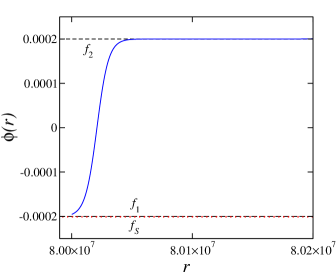
Figure 5: $\phi(r)$ of a solution with $f/M_{{\rm Pl}}=0.0002,f_{r}=0.0002,\lambda=1$, $h_{S}=(f_{1}-f_{S})/f=0.005$ and $R_{1}/l_{{\rm Pl}}=8\times 10^{7}$. $\phi$ and $r$ are in units of $M_{{\rm Pl}}$ and $l_{{\rm Pl}}$, respectively.

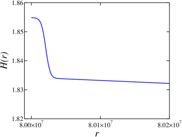
Figure 6: $H(r)$ of a solution with $f/M_{{\rm Pl}}=0.0002,f_{r}=0.0002,\lambda=1$, $h_{S}=(f_{1}-f_{S})/f=0.005$ and $R_{1}/l_{{\rm Pl}}=8\times 10^{7}$. $r$ is in units of $l_{{\rm Pl}}$.

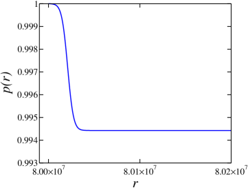
Figure 7: $p(r)$ of a solution with $f/M_{{\rm Pl}}=0.0002,f_{r}=0.0002,\lambda=1$, $h_{S}=(f_{1}-f_{S})/f=0.005$ and $R_{1}/l_{{\rm Pl}}=8\times 10^{7}$. $r$ is in units of $l_{{\rm Pl}}$.

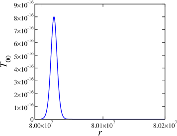
Figure 8: The energy density $T_{00}$ for a solution with $f/M_{{\rm Pl}}=0.0002,f_{r}=0.0002,\lambda=1$, $h_{S}=(f_{1}-f_{S})/f=0.005$ and $R_{1}/l_{{\rm Pl}}=8\times 10^{7}$. $T_{00}$ and $r$ are in the units of $M_{{\rm Pl}}^{4}$ and $l_{{\rm Pl}}$, respectively. For $r<R_{1}$, $T_{00}\sim\epsilon<0$.

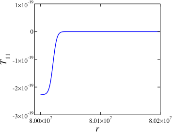
Figure 9: The radial pressure $T_{11}$ for a solution with $f/M_{{\rm Pl}}=0.0002,f_{r}=0.0002,\lambda=1$, $h_{S}=(f_{1}-f_{S})/f=0.005$ and $R_{1}/l_{{\rm Pl}}=8\times 10^{7}$. $T_{11}$ and $r$ are in the units of $M_{{\rm Pl}}^{4}$ and $l_{{\rm Pl}}$, respectively. For $r<R_{1}$, $T_{11}\sim-\epsilon>0$.

(ii) Region II

In region II, $\phi(r)$ varies substantially and the nonlinearity of the equations plays an essential role. In this region the equations must be solved numerically. With fine tuning of the value of $\delta\phi(R_{1})$ nontrivial lump solutions are found.

The algorithm for numerically finding solutions is the following. First $R_{1}$, $\delta\phi(R_{1})$ and $f_{S}$ are chosen and $\delta\phi^{\prime}(R_{1})$ is evaluated using (37) and (39). In this paper we investigate the solutions in the case that $|f_{1}-f_{S}|\ll f$ and the linearization in Region I is valid. To a good approximation the metric is given by $H(R_{1})=1+(R_{1}/a_{f})^{2}$ and $p(R_{1})=1$. With the boundary conditions $\delta\phi(R_{1})$ and $\delta\phi^{\prime}(R_{1})$ the equations are numerically solved in region II. The width of the transition region, $w=R_{2}-R_{1}$ is approximately given by $1/\sqrt{\lambda}\,f$.[7]

The behavior of solutions in region II is displayed in Fig. 5. When the values of the input parameters are chosen to be $\lambda=1$, $f/M_{{\rm Pl}}=0.0002$, $f_{r}=\Delta f/f=0.0002$ and $h_{S}=(f_{1}-f_{S})/f=0.005$, then the output parameters are $\rho_{0}l_{\rm Pl}^{3}=8.0593\times 10^{-14}$, $\epsilon/M_{\rm Pl}^{4}=-1.5944\times 10^{-17}$, $|\epsilon|/\epsilon_{0}=74.738$, $a_{f}/l_{{\rm Pl}}=8.6525\times 10^{7}$ and $\kappa=1.23275\times 10^{4}$. Here $l_{{\rm Pl}}$ is the Planck length. We note that $\rho_{0}/f^{3}=0.0101$, $\epsilon/f^{4}=-0.00997$, and $a_{f}f=17305$. For $R_{1}/l_{{\rm Pl}}=8\times 10^{7}$ ($R_{1}/a_{f}=0.924589$) we find a solution with $\delta\phi(R_{1})/M_{{\rm Pl}}=5.545749\cdots\times 10^{-6}$. In this example, the value of $\delta\phi$ at the origin ($r=0$) is found from Eq. (35) to be $9.5\times 10^{-8857}$, which explains why numerical integration of $\phi(r)$ from $r=0$ to $R_{1}$ is not possible. A small discontinuity in $\phi^{\prime\prime}$ appears at $r=R_{1}$ due to the discontinuous change in $\rho_{S}(r)$.

The field $\phi(r)$ approaches $f_{2}$ for $r>R_{2}$. In the numerical integration $R_{1}$ and $f_{S}$ are kept fixed while $\delta\phi(R_{1})$ is varied. If $\delta\phi(R_{1})$ is taken to be slightly smaller, then $\phi(r)$ starts to deviate from $f_{2}$ in the negative direction, approaching $f_{1}$ as $r$ increases. If $\delta\phi(R_{1})$ is taken to be slightly larger, then $\phi(r)$ overshoots $f_{2}$, diverging to $+\infty$ as $r$ increases. With just the right value of $\delta\phi(R_{1})$, the spacetime becomes nearly flat in region III.

(iii) Region III

The behavior of the solution in region III is easily inferred. From the numerical integration in region II both $H_{2}=H(R_{2})$ and $p_{2}=p(R_{2})$ are determined. In region III the metric can be written in the Schwarzschild form

$$\hskip-28.45274ptH(r)=1-{2G\widetilde{M}\over r}$$ (40)

$$\hskip-28.45274ptp(r)=p_{2}~{}~{},$$ (41)

where $\widetilde{M}$ is the mass of the lump. As $\phi(r)$ approaches its asymptotic value $f_{2}$ and $T_{00}$ vanishes, $H(r)$ must take this form. The value of $\widetilde{M}$ is determined numerically either by integrating $T_{00}$ in Eq. (13), or by fitting $H(r)$ in Eq. (13) just outside the shell. In the numerical example presented above, $\widetilde{M}<0$. As can be seen in fig. 6, $H(r)$ converges to the asymptotic value from above. A rough estimate of $\widetilde{M}$ is

$$\widetilde{M}\sim{4\pi\over 3}R_{1}^{3}~{}\epsilon\sim-{M_{\rm Pl}^{3}\over 10f^{2}\sqrt{\lambda h_{s}}}\bigg{(}{R_{1}\over a_{f}}\bigg{)}^{3}~{}~{}~{}.$$ (42)

5 Scales of the solutions

In the previous section we have solved the linearized field equation for $\phi(r)$ in region I where $\rho_{S}\not=0$ and the deviation from $f_{S}$ was found to be small. We numerically determined the behavior in the nonlinear region II. The resulting structure is a lump with negative mass and fermions at its core. In this section we present more detailed numerical results. As discussed in the previous section the boundary between regions I and II, located at the matching radius $R_{1}$, is rather arbitrary, subject only to the condition that the linearization be accurate up to that radius. Precise tuning is necessary for $R_{1}$ and $\delta\phi(R_{1})$ in order to obtain a lump solution. Technically it is easier to keep $R_{1}$ fixed and adjust $\delta\phi$ at $R_{1}$. If $\delta\phi(R_{1})$ is chosen too small, $\phi$ comes back toward $f_{1}$, but cannot reach it, eventually oscillating about $\phi=0$ as $r$ increases. If $\delta\phi(R_{1})$ is chosen too large, $\phi$ overshoots $f_{2}$ and continues to increase. With just the right value of $\delta\phi(R_{1})$, $\phi$ will approach $f_{2}$. There can appear shell solutions in which $\phi$ goes back to $f_{1}$ at $r=\infty$. Such solutions are discussed in ref. [7].

One example of the lump solutions is displayed in Fig. 5 for the parameter values $f/M_{{\rm Pl}}=0.0002$, $f_{r}=0.0002$, $\lambda=1$ and $h_{S}=(f_{1}-f_{S})/f=0.005$. If we take $R_{1}/l_{\rm Pl}=8\times 10^{7}$ ($R_{1}/a_{f}=0.924589$), $\delta\phi(R_{1})$ musto be fine-tuned to more than 7 digits: $\delta\phi(R_{1})/M_{\rm Pl}\sim 5.545749\cdots\times 10^{-6}$. In the transition region both $H(r)$ and $p(r)$ decrease in a one-step fashion. See Figs. 6 and 7. Inside the lump $H(r)$ is given by (33), whereas outside the lump it is given by

$$H=1-{2G\widetilde{M}\over r}$$ (43)

where $\widetilde{M}/M_{\rm Pl}\approx-3.337\times 10^{7}$ ($\widetilde{M}/f\approx-1.669\times 10^{11}$). $p(r)$ assumes the constant values 1 and 0.9944 inside and outside the lump, respectively.

The behavior of the energy-momentum tensors, $T_{00}=-T_{22}=-T_{33}$ and $T_{11}$, are displayed in Fig. 8 and Fig. 9. The energy density $T_{00}$ has one sharp peak associated with the rapid variation of $\phi$. The radial pressure $T_{11}$ is $\sim-\epsilon>0$ for $r<R_{1}$ and becomes negative at $R_{1}$. It increases to zero quickly, and it remains zero outside the lump. The absolute value of $T_{11}(R_{1})$ in the transition region II is very small ($\sim 2.3\times 10^{-19}M_{{\rm Pl}}^{4}$) compared with the maximum value of $T_{00}$ ($\sim 8\times 10^{-16}M_{{\rm Pl}}^{4}$). The contributions of the kinetic energy, $\hbox{${1\over 2}$}H\phi^{\prime 2}$, and potential energy, $V[\phi]$, almost cancel each other in the transition region.

The model contains several dimensionless parameters, $\lambda$, $f/M_{{\rm Pl}}$, $f_{r}$, $R_{1}/a_{f}$ and $\rho_{0}f^{3}$. When the values of these parameters are varied, the size of the resulting lump solutions also varies. In the numerical evaluation we took values of $f/M_{{\rm Pl}}$ and $f_{r}$ in the range between $10^{-4}$ and $10^{-3}$. It is of great interest to determine the structure of the lump solutions when, for instance, $f/M_{{\rm Pl}}=10^{-19}$. One can obtain insight into this problem by investigating the dependence of the solutions on the above parameters.

In the numerical investigation values of $\lambda$, $f/M_{{\rm Pl}}$, $f_{r}$, $R_{1}/a_{f}$ and $h_{S}$ are given, and we try to find a desired value of $\delta\phi(R_{1})$ for a solution to exist. In Fig. 10, $\delta\phi(R_{1})/|f_{S}|$ is plotted as a function of $f$. It is seen that as $f$ increases, the value of $\delta\phi$ at $R_{1}$ needs to be increased in order to get a lump solution. The numerical evaluation becomes unreliable when $\delta\phi(R_{1})/|f_{S}|$ becomes large and the linearization in Eq. (16) is no longer valid.

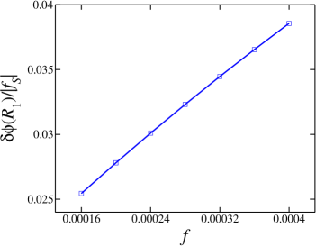
Figure 10: The $f$ dependence of $\delta\phi(R_{1})$. $f_{r}=0.0002$, $R_{1}/a_{f}=0.9$ and $h_{S}=(f_{1}-f_{S})/f=0.005$ are fixed. $f$ is in a unit of $M_{{\rm Pl}}$.

In Fig. 11, $\delta\phi(R_{1})/|f_{S}|$ is plotted as a function of $f_{r}$. We find that $\delta\phi(R_{1})/|f_{S}|$ increases as $f_{r}$ increases. In Fig. 12, $\delta\phi(R_{1})/|f_{S}|$ is plotted versus $R_{1}/a_{f}$. As $R_{1}/a_{f}$ increases, $\delta\phi(R_{1})/|f_{S}|$ decreases and approaches a constant ($\sim 0.022$).

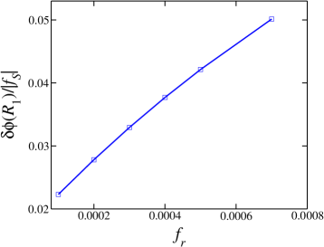
Figure 11: The $f_{r}$ dependence of $\delta\phi(R_{1})$. $f=0.0002$, $R_{1}/a_{f}=0.9$ and $h_{S}=(f_{1}-f_{S})/f=0.005$ are fixed. $f_{r}$ is in a unit of $M_{{\rm Pl}}$.

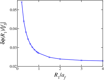
Figure 12: The $R_{1}$ dependence of $\delta\phi(R_{1})$. $f/M_{{\rm Pl}}=0.0002$, $f_{r}=0.0002$ and $h_{S}=(f_{1}-f_{S})/f=0.005$ are fixed.

In Fig. 13, $\delta\phi(R_{1})/|f_{S}|$ is plotted versus $h_{S}$. In this figure $\delta\phi(R_{1})/|f_{S}|$ decreases as $h_{S}$ increases and then it begins to increase when $h_{S}$ becomes greater than approximately $0.015$. The reason for the increase in the value of $\delta\phi(R_{1})/|f_{S}|$ is that at some point $|f_{S}-f_{1}|$ becomes greater than $\delta\phi(R_{1})$, which means that $\phi(R_{1})<f_{1}$. In this situation the solution will diverge to negative infinity if we do not take $\delta\phi(R_{1})$ large enough. In fig. 14 $R_{1}$ is plotted as a function of $f$ with other parameters, including $\delta\phi(R_{1})/|f_{S}|$, kept fixed.

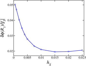
Figure 13: The $h_{S}$ dependence of $\delta\phi(R_{1})$. $f/M_{{\rm Pl}}=0.0002$, $f_{r}=0.0002$ and $R_{1}/a_{f}=0.9$ are fixed.

With the above results we can obtain good information concerning the mass $\widetilde{M}$ of the lumps. In Figs. 15 and 16 $\widetilde{M}$ is plotted as a function of $f$ and $R_{1}$, respectively. We find that the estimate (42) is good. As an example, let us take $f_{r}=0.0002$, $h_{S}=0.005$, $\lambda=0.01$, and $g=1$. Then $a_{f}\sim 1.2\cdot 10^{5}\cdot(1\,{\rm GeV}/f)^{2}\,{\rm m}$ and $-\widetilde{M}\sim 4.6\cdot 10^{31}\cdot(1\,{\rm GeV}/f)^{2}\,(R_{1}/a_{f})^{3}\,{\rm kg}$. As $f$ becomes small, the size of the lump becomes very large.

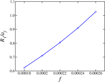
Figure 14: $R_{1}$ versus $f$. $f_{r}=0.0002$, $h_{S}=(f_{1}-f_{S})/f=0.005$ and $\delta\phi(R_{1})/|f_{S}|=0.03$ are fixed. $f$ is in a unit of $M_{{\rm Pl}}$.

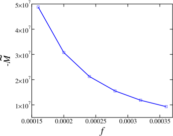
Figure 15: $\widetilde{M}$ versus $f$. $f_{r}=0.0002$, $h_{S}=(f_{1}-f_{S})/f=0.005$ and $R_{1}/a_{f}=0.9$ are fixed. $f$ and $\widetilde{M}$ are in a unit of $M_{{\rm Pl}}$.

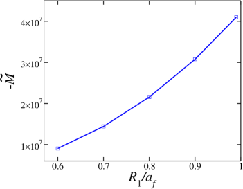
Figure 16: $\widetilde{M}$ versus $R_{1}$. $f/M_{{\rm Pl}}=0.0002$, $f_{r}=0.0002$ and $h_{S}=0.005$ are fixed. $\widetilde{M}$ is in a unit of $M_{{\rm Pl}}$.

6 Discussion

In this paper we have demonstrated that there exist fermionic gravitating lumps with a false vacuum core of the scalar field. This is a curious structure which may appear at various scales. We have constructed lump solutions for the case $h_{S}=(f_{1}-f_{S})/f>f_{r}=(f_{2}-|f_{1}|)/f$, which implies that $\lambda f_{r}/g<\rho_{n}/2f^{3}\ll g^{3}$. (See Eq. (27).) If the typical energy scale is very high, the size of the lump will be small but it can be produced abundantly in the early universe. If the energy scale becomes low, this size may increases to a cosmic scale.

We have focused on the cases in which fermion contributions or back-reaction to the metric is small. Certainly this restriction needs to be relaxed in order to accommodate more realistic models in the particle theory. The lump solutions presented in this paper have negative masses as seen outside the lumps. As the mass and density of fermions inside the lump increase, the mass of the lump will become positive. The solution probably continues to exist in this case, though explicit construction of such a solution is necessary by taking account of the back-reaction to the energy-momentum tensors. An investigation along this line is in progress, and we hope to report it in the near future.

A false vacuum state may appear in the standard model of electroweak and gravitational interactions. In ref. 17) it is shown that the false vacuum of the Higgs field emerges in the early universe as a result of the winding of the gauge fields in the $S^{3}\times R^{1}$ Robertson-Walker spacetime. As quarks and leptons have relevant Yukawa couplings to the Higgs field, gravitating lumps with quarks and leptons at the core may be copiously produced. As the universe expands, the barrier separating the false vacuum from the true vacuum disappears so that the gravitating fermionic lumps would become unstable, the fermions inside the lumps dissipating to infinity. It is of great interest to elucidate the consequences of this process.

Furthermore, in the higher-dimensional gauge theory defined on orbifolds, false vacua naturally appear in the gauge field configurations.[20] It would be interesting to investigate if the gauge interactions of fermions produce gravitating lumps, as we have found for the Yukawa interactions.

References

[1]
S. Coleman, Phys. Rev. D15 (1977), 2929;
C. G. Callan and S. Coleman, Phys. Rev. D16 (1977), 1762;
S. Coleman and F. De Luccia, Phys. Rev. D21 (1980), 3305.
[2]
R.G. Daghigh, J.I. Kapusta, and Y. Hosotani, gr-qc/0008006.
[3]
Y. Hosotani, Soryushiron Kenkyu
103 (2001) E91, hep-th/0104006.
[4]
A.K. Blau, E.I. Guendeman, and A.H. Guth,
Phys. Rev. D35 (1987), 1747
[6]
M.S. Volkov and D.V. Gal’tsov, Phys. Rep.319 (1999), 1;
D.V. Gal’tsov, hep-th/0112038.
[7]
Y. Hosotani, T. Nakajima, R. G. Daghigh and J. I. Kapusta,
Phys. Rev. D66 (2002), 104020, gr-qc/0112079.
[8]
S. Coleman, Nucl. Phys. B262 (1985), 263;
A. Kusenko, Phys. Lett. B404 (1997), 285;
A. Kusenko and M.E. Shaposhnikov, Phys. Lett. B418 (1998), 46.
[9]
D.J. Kaup, Phys. Rev.172 (1968), 1331;
E.W. Mielke and R. Scherzer, Phys. Rev. D24 (1981), 2111;
M. Colpi, S.L. Shapiro and I. Wasserman,
Phys. Rev. Lett. 57 (1986), 2485;
A. Iwazaki, Phys. Rev. D60 (1999), 025001;
E.W. Mielke and F.E. Schunck, Phys. Rev. D66 (2002), 023503.
[10]
R. Ruffini and S. Bonazzola, Phys. Rev.187 (1969), 1767;
E. Takasugi and M. Yoshimura, Z. Phys. C26 (1984), 241;
M. Gleiser, Phys. Rev. D38 (1988), 2376;
P. Jetzer, Phys. Rep.220 (1992), 163.
[11]
A. L. Macpherson and B.A. Campbell, Phys. Lett. B347 (1995), 205;
J.R. Morris, Phys. Rev. D59 (1998), 023513.
[12]
T. Yoshida, K. Ogure, and J. Arafune, Phys. Rev. D67 (2003), 083506;
Phys. Rev. D68 (2003), 023519;
K. Ogure, T. Yoshida, and J. Arafune, Phys. Rev. D67 (2003), 123518.
[13]
E. Winstanley, Class. Quant. Grav. 16 (1999), 1963;
J. Bjoraker and Y. Hosotani, Phys. Rev. Lett. 84 (2000), 1853;
Phys. Rev. D62 (2000), 043513;
E. Radu, Phys. Rev. D65 (2002), 044005; Phys. Rev. D67 (2003), 084030;
J.J. van der Bij and E. Radu, Phys. Lett. B536 (2002), 107;
Y. Hosotani, J. Math. Phys.43 (2002), 597.
P. Breitenlohner, D. Maison, and G. Lavrelashvili,
gr-qc/0307029 ;
D.H. Correa, E.F. Moreno, A.D. Medina, and F.A. Schaposnik,
hep-th/0307080.
[14]
R. Bartnik and J. McKinnon, Phys. Rev. Lett. 61 (1988), 141;
H. Künzle and A. Masood-ul-Alam, J. Math. Phys.31 (1990), 928.
[15]
T. Torii, K. Maeda, and T. Tachizawa,
Phys. Rev. D52 (1995), 4272;
M.S. Volkov, N. Straumann, G.V. Lavrelashvili, M. Heusler
and O. Brodbeck, Phys. Rev. D54 (1996), 7243.
[16]
I. Dymnikova, gr-qc/0010016.
[17]
H. Emoto, Y. Hosotani, and T. Kubota,
Prog. Theoret. Phys. 108 (2002), 157, hep-th/0201141;
Y. Hosotani, H. Emoto, and T. Kubota,
Proc. Int. Conf. High Energy Phys. 2002, pp. 139, hep-ph/0209112.
[18]
Masafumi Hashimoto, Master’s Thesis, submitted to Osaka University,
February 2001.
[20]
N. Haba, M. Harada, Y. Hosotani and Y. Kawamura, Nucl. Phys. B657 (2003), 169,
Errata; B669 (2003) 381,
hep-ph/0212035;
Y. Hosotani, in ”Strong Coupling Gauge Theories and Effective Field Theories”,
ed. M. Harada, Y. Kikukawa and K. Yamawaki (World Scientific 2003), p. 234. hep-ph/0303066.