Perturbations of global monopoles as a black hole’s hair

Abstract

We study the stability of a spherically symmetric black hole with a global monopole hair. Asymptotically the spacetime is flat but has a deficit solid angle which depends on the vacuum expectation value of the scalar field. When the vacuum expectation value is larger than a certain critical value, this spacetime has a cosmological event horizon. We investigate the stability of these solutions against the spherical and polar perturbations and confirm that the global monopole hair is stable in both cases. Although we consider some particular modes in the polar case, our analysis suggests the conservation of the “topological charge” in the presence of the event horizons and violation of black hole no-hair conjecture in asymptotically non-flat spacetime.

1 Introduction

The exterior gravitational field of a stationary source may have a large number of independent multipole moments. However, if a black hole event horizon (BEH) is formed, these multipole moments will reduce to three physical parameters, $M$, $a$ and $Q$. These parameters are interpreted as mass, angular momentum and net electromagnetic charge of the black hole, respectively. This statement is called the black hole no-hair conjecture, which was proposed by Ruffini and Wheeler[1].

Many candidates for counter-examples were proposed to investigate whether this conjecture is true or not. Among them the colored black hole in Einstein-Yang-Mills system is interesting[2]. Although this solution is unstable[3], it opened up a new possibility that the black hole may have various matter hairs[4]. Actually stable non-Abelian black hole solutions were found as the black hole counter-part of the self-gravitating topological defects and solitons[5, 6].

Another possibility for the hairy black hole is the solution in asymptotically non-flat spacetime. One of us showed that the black hole can support a scalar hair in asymptotically de Sitter[7] and anti-de Sitter spacetime[8]. The colored black hole in anti-de Sitter spacetime was also reported[9]. Some of these solutions were found to be stable, so they can be strong counter-examples to the black hole no-hair conjecture.

Phase transitions in the early universe are caused by symmetry breaking leading to a manifold of degenerate vacua with nontrivial topology and giving rise to topological defects. The topological defects are classified into domain walls, cosmic strings and monopoles by the topology of the vacua. If the gauge field is involved in the spontaneous symmetry breaking, the topological defects are gauged. On the other hand, when the symmetry is global, the emerging defects are called global defects.

Although energy of the gauge monopole is finite, the global monopole has divergent energy because of the long tail of the scalar field. This divergence has to be removed by cutting it off at a certain distance. This procedure is not necessarily artificial in the early universe, because other defects which may exist near the original one cancel the divergence. These neighboring defects are not only the monopoles, but also can be domain walls or cosmic strings.

When general relativistic self-gravity is considered, such a divergent behavior can be made to disappear by a new definition of the energy[10]. Spacetime becomes asymptotically flat but has a deficit solid angle[11]. Moreover, the motion of a test particle around the global monopole perceives repulsive force from the center[12].

This kind of global monopole has a different asymptotic behavior from the non-gravitating one[13]. As the vacuum expectation value (VEV) $v$ of the $O(3)$ scalar field increases, the deficit solid angle also gets large and becomes $4\pi$ when $v=v_{cri}:=\sqrt{1/8\pi}\approx 0.199$. Beyond this critical value there is no ordinary monopole solution, but a new type of solution appears in the parameter range $v_{cri}<v<v_{max}:=\sqrt{3/8\pi}\approx 0.345$. This has a cosmological event horizon (CEH) at $r=r_{c}$. We call this the supermassive global monopole in imitation of the supermassive global strings[14]. When $v>v_{max}$, there are only trivial de Sitter solutions under the hedgehog ansatz. This solution has a configuration where the scalar field sits on the top of the potential barrier.

One of the most important issues for these kinds of isolated objects is stability. In the non-gravitating monopole case, if Derrick’s no-go theorem[15] could be applied, they would be unstable towards a radial rescaling of the field configuration. This is, however, not the case due to the diverging energy of the solutions. It was demonstrated that the monopole solutions are stable against spherical perturbations. As for the non-spherical perturbations, several studies have been done. Consequently, the non-gravitating global monopole is stable against both spherical and polar perturbations. That is consistent with the conservation of the topological charge.

In the self-gravitating case, the global monopole can have a CEH. Thus we can not define exact topological charges because of the peculiar asymptotic structure. One may find an exact proof of the conservation of the “topological charges” defined by the analogy even in the spacetime with the BEH and/or CEH by putting the in-going and/or out-going conditions at each horizon. This issue is very interesting but beyond the scope of the current paper.

Maison and Liebling studied the stability of the static solution against spherical and hedgehog type perturbations[16]. They found that the supermassive monopole and de Sitter solutions are stable when $v<v_{max}$. We investigated the stability against polar perturbations[17], without the spherical symmetry nor the hedgehog ansatz. We obtained the conclusion that the (supermassive) monopole solution is stable while the de Sitter solution is always unstable.

If a black hole collides with and absorbs a global monopole, the black hole would have $O(3)$ scalar hair. This type of solution was found numerically[13]. The spacetime of this solution is asymptotically flat but with a deficit solid angle or has the CEH. There emerges a question of whether the black hole no-hair conjecture holds in such a spacetime. This is the issue of this paper.

This paper is organized as follows. In Sec. 2, we introduce the model and review the global monopole and the black hole solutions. In Sec. 3, we analyze the spherical perturbation of the solutions. In Sec. 4, we formulate the polar perturbations of the $O(3)$ scalar field and the metric, and show the stability of the black hole with global monopole hair. Throughout this paper, we use the units $\hbar=c=G=1$.

2 Black hole solution with the global monopole hair

In this section, we briefly review the self-gravitating global monopole solution[11, 16] and its black hole counter-part. We consider a scalar field which has spontaneously broken internal $O(3)$ symmetry, and minimally couples to gravity. The action is

$$S=\int d^{4}x\sqrt{-g}\left[\frac{R}{16\pi}-\frac{1}{2}\partial_{\mu}\Phi^{a}\partial^{\mu}\Phi^{a}-\frac{\lambda}{4}\bigl{(}\Phi^{2}-v^{2}\bigr{)}^{2}\right],$$ (1)

where $R$ is the Ricci scalar of the spacetime and $\Phi^{a}$ $(a=1,2,3)$ is the triplet scalar field. $\lambda$ and $v$ are the self-coupling constant and the VEV of the scalar field, respectively. The energy momentum tensor is

$$T_{\mu\nu}=\partial_{\mu}\Phi^{a}\partial_{\nu}\Phi^{a}-g_{\mu\nu}\left[\frac{1}{2}\partial_{\rho}\Phi^{a}\partial^{\rho}\Phi^{a}+\frac{\lambda}{4}\bigl{(}\Phi^{2}-v^{2}\bigr{)}^{2}\right].$$ (2)

For a static solution with unit winding number, we adopt the so-called hedgehog ansatz to the scalar field,

$$\Phi^{a}=h(t,r)\frac{x^{a}}{r},$$ (3)

where $x^{a}$ are the Cartesian coordinates. We shall consider spherically symmetric static spacetime,

$$ds^{2}=-f(r)e^{-2\delta(r)}dt^{2}+\frac{1}{f(r)}dr^{2}+r^{2}(d\theta^{2}+\sin^{2}\theta d\phi^{2}),$$ (4)

where

$$f(r)=1-\frac{2m(r)}{r}.$$ (5)

By scaling the variables as

$$\bar{x}^{\mu}=v\sqrt{\lambda}x^{\mu},\,\,\,\,\bar{m}=v\sqrt{\lambda}m,\,\,\,\,\bar{h}=\frac{h}{v},\,\,\,\,\bar{\Phi}=\frac{\Phi}{v},$$ (6)

the action can be rewritten as

$$S=\int d^{4}x\sqrt{-g}\left[\frac{\bar{R}}{16\pi v^{2}}-\frac{1}{2}\partial_{\mu}\bar{\Phi}^{a}\partial^{\mu}\bar{\Phi}^{a}-\frac{1}{4}\bigl{(}\bar{\Phi}^{2}-1\bigr{)}^{2}\right].$$ (7)

In this formula, the coupling constant $\lambda$ is scaled out. The VEV appears only in the denominator of the curvature term and affects the system only when self-gravity is taken into account. The basic equations are

$$\frac{dm}{dr}=4\pi v^{2}r^{2}\left[\frac{1}{2}fh^{\prime 2}+\frac{h^{2}}{r^{2}}+\frac{1}{4}(h^{2}-1)^{2}\right],$$ (8)

$$\frac{d\delta}{dr}=-4\pi v^{2}r{h^{\prime}}^{2},$$ (9)

$$\bigl{(}r^{2}e^{-\delta}fh^{\prime}\bigr{)}^{\prime}-2he^{-\delta}=r^{2}e^{-\delta}(h^{2}-1)h,$$ (10)

where a prime denotes a derivative with respect to the radial coordinate. We have omitted the bar of the variables.

We integrate these equations with suitable boundary conditions. If we put the regularity condition at the center, we will obtain the self-gravitating monopole solution. In the black hole case the spacetime and the scalar field should be regular at the BEH. By this condition we find $h$ at BEH ($r=r_{b}$) can be regarded as a free parameter and the other variables are determined by $h(r_{b})$. We choose $\delta(r_{b})=0$. Then $\delta$ approaches some constant value $\delta_{\infty}$ as $r\to\infty$. The ordinary asymptotic metric is recovered by rescaling the time coordinate as $t:=te^{-\delta_{\infty}}$. The free parameter $h(r_{b})$ is determined by the other boundary conditions at $r\rightarrow\infty$ for the spacetime without the CEH or at the CEH ($r=r_{c}$) for the supermassive case.

Whether the self-gravitating monopole and the monopole black hole have the CEH or not depends on the VEV. When $0<v<v_{cri}$, the spacetime does not have the CEH. The configuration of the scalar field and the metric are shown in Fig. 1 (solid lines). For the case in which the VEV is larger than the critical value $v_{cri}$, the spacetime has the CEH. In Fig. 1 we can also see this feature (dashed line). There is the maximum value $v_{max}$ where the supermassive global monopole (BH) solution coincides with the (Schwarzschild-)de Sitter solution. Beyond $v_{max}$ no non-trivial solution exists.

For the regular monopole case without the BEH Maison and Liebling investigated the stability against the spherical (both in spacetime and in internal space) perturbations. They found that both the ordinary and the supermassive monopole solutions are stable. We extended their analysis and investigated the stability against the polar perturbations. We found that both of monopole solutions are stable while the de Sitter solution is always unstable[17].

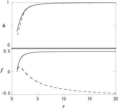
Figure 1: The configurations of the scalar field $h$ and metric function $f$ of the monopole black hole for $v=0.15<v_{cri}$ (solid line: the ordinary case) and $v=0.25>v_{cri}$ (dashed line: the supermassive case). We fix $r_{b}=1.0$. In the ordinary case, the metric function $f$ approaches a constant value less than $1$ as $r\rightarrow\infty$. This means that the spacetime has a deficit solid angle. For the supermassive case, the metric function $f$ crosses zero at the CEH.

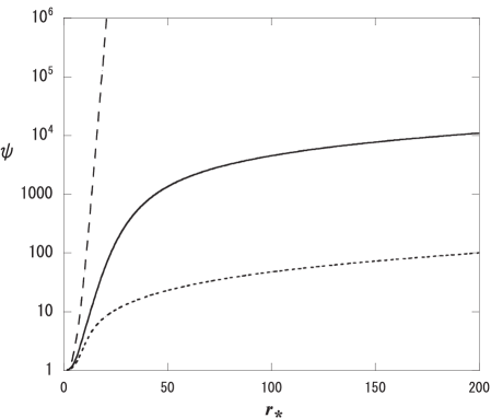
Figure 2: The configurations of the integrated function for $v=0.15$ (dashed line), $v=0.25$ (solid line) and $v=0.28$ (doted line) with $\sigma^{2}=0$. They do not have a node but are positive definite outside of the BEH. This indicates nonexistence of the unstable modes.

3 Spherical perturbation of the global monopole hair

In the remainder of this paper, we investigate the stability of the black hole solutions with the ordinary and the supermassive global monopole hair. Since our solutions have event horizons, the “topological charge” may not be conserved. So our analysis is interesting from the view point of the defects in spacetime with horizons. This issue is also interesting in relation to the black hole hair.

The metric perturbations which we adopt here are,

$$m(r)\rightarrow m(r)+\tilde{m}(r)e^{i\sigma t},$$ (11)

$$\delta(r)\rightarrow\delta(r)+\tilde{\delta}(r)e^{i\sigma t}.$$ (12)

The the perturbation of the scalar field is

$$h(r)\rightarrow h(r)+\tilde{h}(r)e^{i\sigma t}.$$ (13)

We introduce new variable $\psi$,

$$\tilde{h}(r)=\frac{\psi(r)}{r}.$$

Then the perturbation equations becomes a Schrödinger type equation as follows,

$$-\frac{d^{2}\psi}{dr_{*}^{2}}+U(r)\psi=\sigma^{2}\psi,$$ (14)

where $r_{*}$ is the tortoise coordinate ($d/dr_{*}=fe^{-\delta}d/dr$) and

$$U(r)=e^{2\delta}f\left[\frac{f^{\prime}}{r}-4\pi v^{2}fh^{\prime 2}\biggl{(}1+2r\frac{f^{\prime}}{f}+8\pi v^{2}h^{2}\biggr{)}\right.$$

$$\left.+\frac{2}{r^{2}}+16\pi rv^{2}\biggl{(}\frac{2}{r^{2}}+h^{2}-1\biggr{)}hh^{\prime}+3h^{2}-1\right].$$ (15)

As the boundary conditions of the perturbation functions, we assume the in-going boundary conditions at the BEH. Although, one usually puts out-going boundary condition at infinity to calculate quasi-normal modes of an isolated object, we leave it free as long as the perturbation functions do not diverge because we are not interested in the definite quasi-normal modes but in the stability. If we put the out-going boundary condition, which is more restricted condition than ours, and there are unstable modes, these modes are also found out by our analysis.

What we will do is search the unstable mode by integrating Eq. (14) for various value of $\sigma$. As a result, we could not find any unstable modes similar to the self-gravitating monopole analyzed by Maison and Liebling[16].

Although our numerical analysis does not give exact proof of the non-existence of the unstable modes, we can show a basis for stability.

Fig. 2 is the configurations of the integrated function with $\sigma^{2}=0$. If this function has at least one node, we would find the unstable modes. However, the function with any $v$ does not have a node but is positive definite outside of the BEH. Thus we may conclude that the static solutions are stable against spherical perturbations.

4 Polar perturbation of the global monopole hair

Several studies have been made on the non-spherical perturbations of the non-gravitating global monopole[18, 19, 20]. Goldhaber proposed the polar deformation of the $O(3)$ scalar field,

$$\Phi^{1} = H(t,r,\theta)\sin\tilde{\theta}(t,r,\theta)\cos\phi,$$

$$\Phi^{2} = H(t,r,\theta)\sin\tilde{\theta}(t,r,\theta)\sin\phi,$$ (16)

$$\Phi^{3} = H(t,r,\theta)\cos\tilde{\theta}(t,r,\theta),$$

where

$$\tan\biggl{(}\frac{\tilde{\theta}}{2}\biggr{)}=e^{\Theta+\delta\Theta(t,r,\theta)},$$ (17)

$\tilde{\theta}$ is the polar component of $\Phi^{a}$, $\Theta\!:=\ln[\tan(\theta/2)]$ and $H(t,r,\theta)=h(r)+\delta h(t,r,\theta)$. When $\delta\Theta\equiv 0$, i.e., $\tilde{\theta}\equiv\theta$ and $\delta h\equiv\delta h(t,r)$, the global monopole is spherically symmetric, while it become a “string” along the $z$-axis when $\delta\Theta\rightarrow\infty$. The energy of the static global monopole is expressed with the new coordinate $\Theta$,

$$E = \int drd\Theta d\phi(\rho_{1}+\rho_{2}),$$ (18)

where

$$\rho_{1} = \frac{H^{2}}{2}\biggl{[}\sin^{2}\tilde{\theta}+\biggl{(}\frac{\partial\tilde{\theta}}{\partial\Theta}\biggr{)}^{2}+\frac{r^{2}}{\cosh^{2}\Theta}\biggl{(}\frac{\partial\tilde{\theta}}{\partial r}\biggr{)}^{2}\biggr{]},$$

$$\rho_{2} = \frac{1}{2}\biggl{(}\frac{\partial H}{\partial\Theta}\biggr{)}^{2}+\frac{r^{2}}{2\cosh^{2}\Theta}\biggl{[}\biggl{(}\frac{\partial H}{\partial r}\biggr{)}^{2}+\frac{1}{2}(H^{2}-1)^{2}\biggr{]}.$$ (19)

In the far region from the monopole core, the terms $\partial H/\partial r$ and $\partial H/\partial\Theta$ can be neglected. Similarly one can neglect $\partial\tilde{\theta}/\partial r$ and $(H^{2}-1)$ (See Ref. [18] for details). Goldhaber pointed out that the remaining first two terms in $\rho_{1}$ have the same form as the energy of a sine-Gordon soliton, which implies that the energy is invariant under translation of coordinate $\Theta$ (or $\xi$).

We adopt Goldhaber’s formula to investigate the stability of the black hole with a global monopole hair. We consider the simplest case,

$$\Phi^{1} = \Bigl{[}h+(\eta+h\xi)\cos\theta e^{i\sigma t}\Bigr{]}\sin\theta\cos\phi,$$

$$\Phi^{2} = \Bigl{[}h+(\eta+h\xi)\cos\theta e^{i\sigma t}\Bigr{]}\sin\theta\sin\phi,$$ (20)

$$\Phi^{3} = \Bigl{[}h+(\eta+h\xi)\cos\theta e^{i\sigma t}\Bigr{]}\cos\theta-h\xi e^{i\sigma t},$$

where $\delta\Theta=\xi(r)e^{i\sigma t}$ and $\delta h=\eta(r)\cos\theta e^{i\sigma t}$. This corresponds to the polar perturbation with $l=1$. In this paper we consider only the $l=1$ case because the perturbation corresponding to $l\geq 2$ of Goldhaber’s formula are so complicated that explicit forms of them, like orthogonal functions, have not been known.

Since the matter field of the background solution is non-zero, the first order perturbations of the matter field produce the metric perturbations at the first order level, which can be described as

$$ds^{2} = -fe^{-2\delta}e^{\delta\nu}dt^{2}+\frac{1}{f}e^{\delta\mu_{2}}dr^{2}+r^{2}e^{\delta\mu_{3}}d\theta^{2}+r^{2}\sin^{2}\theta e^{\delta\psi}d\phi^{2}.$$ (21)

The first order variables in the metric can be separated [21],

$$\delta\nu = \sum N_{l}(t,r)P_{l}(\cos\theta),$$

$$\delta\mu_{2} = \sum L_{l}(t,r)P_{l}(\cos\theta),$$

$$\delta\mu_{3} = \sum[T_{l}(t,r)P_{l}(\cos\theta)+S_{l}(t,r)P_{l,\theta,\theta}(\cos\theta)],$$

$$\delta\psi = \sum[T_{l}(t,r)P_{l}(\cos\theta)+S_{l}(t,r)P_{l,\theta}(\cos\theta)\cot\theta],$$ (22)

where $P_{l}$ is a Legendre polynomial. Considering the simplest case $l=1$, which is consistent with $l=1$ Goldhaber’s formula, we drop the suffix $l$. Thus, the perturbed metric can be written in the form,

$$ds^{2} = -\left[f+B(r)e^{i\sigma t}\cos\theta\right]e^{-2\delta}dt^{2}+\frac{1}{f}\left[1+L(r)e^{i\sigma t}\cos\theta\right]dr^{2}$$ (23)

$$+r^{2}\left[1+T(r)e^{i\sigma t}\cos\theta\right](d\theta^{2}+\sin^{2}\theta d\phi^{2}).$$

Here, we have introduced a new variable $B(r):=N(r)f(r)$ for convenience, re-defined $T:=T-S$ and assumed harmonic time dependence.

We can get the perturbation equations

$$L+T=16\pi v^{2}h^{2}\xi,$$ (24)

$$-(rT)^{\prime}+r\biggl{(}\frac{f^{\prime}}{2f}-\delta^{\prime}\biggr{)}T+L=8\pi v^{2}rh^{\prime}\eta,$$ (25)

$$\frac{\sigma^{2}e^{2\delta}r^{2}T}{f}-f\biggl{(}1+\frac{rf^{\prime}}{f}-2r\delta^{\prime}\biggr{)}L-\frac{1}{f}(1+rf^{\prime})B+rB^{\prime}+rf\biggl{(}1+\frac{rf^{\prime}}{2f}-r\delta^{\prime}\biggr{)}T^{\prime}$$

$$~{}~{}~{}~{}~{}~{}~{}~{}~{}=8\pi v^{2}\biggl{[}fr^{2}h^{\prime}\eta^{\prime}+h^{2}T-2h(\eta+h\xi)-r^{2}(h^{2}-1)h\eta-\frac{1}{2}fr^{2}{h^{\prime}}^{2}L\biggr{]},$$ (26)

from the Einstein equations and

$$\frac{\sigma^{2}e^{2\delta}h\xi}{f}+f(h\xi)^{\prime\prime}+f\left(\frac{2}{r}+\frac{f^{\prime}}{f}-\delta^{\prime}\right)(h\xi)^{\prime}$$

$$~{}~{}~{}~{}~{}-\frac{2\eta+2h\xi}{r^{2}}+\frac{hL}{2r^{2}}-\frac{hB}{2fr^{2}}-h(h^{2}-1)\xi=0,$$ (27)

$$\frac{\sigma^{2}e^{2\delta}}{f}\eta+f\eta^{\prime\prime}+f\left(\frac{2}{r}+\frac{f^{\prime}}{f}-\delta^{\prime}\right)\eta^{\prime}+fh^{\prime}T^{\prime}-\left[\frac{2h}{r^{2}}+h(h^{2}-1)\right]L$$

$$~{}~{}~{}~{}~{}~{}-\frac{4h\xi+4\eta-2hT}{r^{2}}-\frac{fh^{\prime}L^{\prime}}{2}+\frac{h^{\prime}B^{\prime}}{2}-\frac{h^{\prime}f^{\prime}B}{2f}-(3h^{2}-1)\eta=0,$$ (28)

from the scalar field equation.

We assume the behavior of the variables near $r=r_{b}$ to satisfy the regularity condition as,

$$A=A_{0}+A_{1}\rho+\frac{1}{2}A_{2}\rho^{2}+\dots,$$ (29)

for the background variables such as $m$, $\delta$ and $h$, and

$$A=\rho^{\beta}\biggl{(}A_{0}+A_{1}\rho+\frac{1}{2}A_{2}\rho^{2}+\dots\biggr{)},$$ (30)

for the first order variables such as $B$, $L$, $T$, $\cdots$, where $\rho:=(r-r_{b})/r_{b}$.

Expanding the first order equations (24)-(28) with the Eqs. (29) and (30), we get,

$$\eta_{0}=B_{0}=T_{0}=0,$$ (31)

$$L_{0}=16\pi v^{2}h_{0}\alpha_{0},$$ (32)

$$\alpha_{1} = \Delta\Bigl{\{}2\bigl{[}(1+\delta_{1})(r_{b}-2m_{1})+2m_{2}\bigr{]}{\beta}^{2}+\bigl{[}(\delta_{1}-1)(r_{b}-2m_{1})+2m_{2}\bigr{]}{\beta}$$ (33)

$$~{}~{}~{}~{}~{}~{}~{}~{}+(r_{b}^{2}+16\pi v^{2})h_{0}^{2}r_{b}+2r_{b}^{2}-r_{b}^{3})\Bigr{\}},$$

$$\eta_{1}=4\,\Delta r_{b}\left(4r_{b}^{2}h_{0}^{2}\pi v^{2}(h_{0}^{2}-1)+8h_{0}^{2}\pi v^{2}+1\right),$$ (34)

$$L_{1} = 16\pi\,{v}^{2}\Delta\Bigl{\{}2h_{0}\bigl{[}(1+\delta_{1})(r_{b}-2m_{1})+2m_{2}\bigr{]}{\beta}^{2}$$ (35)

$$~{}~{}~{}~{}~{}~{}+\bigl{[}(r_{b}-2m_{1})\bigl{(}2h_{1}-h_{0}(1-\delta_{1})\bigr{)}+2h_{0}m_{2}\bigr{]}\beta$$

$$~{}~{}~{}~{}~{}~{}+(r_{b}-2m_{1})h_{1}+h_{0}^{3}r_{b}(r_{b}^{2}+16\pi{v}^{2})+h_{0}(4m_{1}-r_{b}^{3})\Bigr{\}},$$

$$B_{1}=16\pi v^{2}\frac{r_{b}-2m_{1}}{r_{b}}h_{0}\alpha_{0},$$ (36)

$$T_{1}=\frac{32\pi v^{2}h_{0}\alpha_{0}}{1+2\beta},$$ (37)

$$\beta^{2}=-\frac{r_{b}^{2}\sigma^{2}}{(1-\frac{2m_{1}}{r_{b}})^{2}},$$ (38)

where $\alpha:=h\xi$ and

$$\Delta:=\frac{\alpha_{0}}{(2\beta+1)(r_{b}-2m_{1})}.$$ (39)

Since now $A_{i}$ of background fields are obtained from the static solution, these equations are relations between the expansion coefficients $A_{i}$ of the perturbed fields. We find that all $A_{i}$ are specified by a value $\xi_{0}$. Hence, $\xi_{0}$ on the BEH are the shooting parameters of this equation system. Our aim is to find an unstable mode or to indicate the non-existence of it. The unstable mode can be assumed to have a real negative $\sigma^{2}$. Therefore we assumed $\sigma^{2}$ is real and focused only on the real part of the perturbation equations.

5 Results and discussion

Having specified the boundary condition at the BEH, we can now integrate the Eqs. (24)-(28) numerically. For the ordinary case, we find the critical value $\sigma^{2}_{min}>0$ below which there is no finite solution. Since we have not put the strict boundary conditions at $r=\infty$ such as the out-going condition but just the regularity condition as in the spherical perturbation case, these modes becomes continuous.

The existence of the critical eigenvalue can be understood from the asymptotic form of Eq. (28) at $r\rightarrow\infty$,

$$-\frac{d^{2}\eta}{dr_{*}^{2}}+fe^{-2\delta}(3h^{2}-1)\eta=\sigma^{2}\eta.$$ (40)

$\eta$ decouples to the other first order variables and is described by a single Schrödinger type equation. The potential $U(r):=fe^{-2\delta}(3h^{2}-1)\to 2fe^{-2\delta_{\infty}}$ approaches a positive value . Hence $\sigma^{2}_{min}$ is determined by the asymptotic value of the potential function as $\sigma^{2}_{min}\simeq 2fe^{-2\delta_{\infty}}$.

It is almost impossible to show the stability of the solution exactly by numerical analysis because of the infiniteness of the phase space of the perturbation function. However, the behavior of the variables with $\sigma^{2}=0$ gives some information about the stability. We find that they have no node as in the spherical case, which suggest that the solution be stable against at least the present polar perturbations.

For the supermassive case, the above potential term vanishes at $r=r_{c}$. Assuming the same boundary conditions as the ordinary case at $r=r_{b}$, we find $\sigma_{min}^{2}=0$ below which no finite solution exists. We find that some of the variables can have a node when $\sigma^{2}=0$. However, we also find that there is no negative $\sigma^{2}$ which makes all variables finite. Moreover, if $\sigma^{2}$ is smaller than some negative value, all variables diverge without node. Thus we conclude that the supermassive case is stable against the present polar perturbations, too.

We investigated the stability of black hole solutions in the Einstein-$O(3)$ scalar system by linear perturbation. The black holes are stable against spherical perturbation as the particle-like case without BEH. We also studied the polar perturbation since the trivial (Schwarzschild) de-Sitter solution with $v_{max}<v$ is stable against the spherical perturbation[16] but not against the non-spherical perturbations[17]. We suggested that the black holes with the ordinary or the supermassive global monopole hair be stable against our perturbations. This result implies that if these kind of objects were formed in the early universe, they can survive without decaying to other object nor swallowing the outer matter field leaving a vacuum black hole. It should be also stressed that the black hole no-hair conjecture is violated for $O(3)$ scalar hair and gives new insight on the problem of black hole hair.

References

References

- [1] R. Ruffini and J. Wheeler, Phys. Today 24(1), 30 (1971).
- [2] M. S. Volkov and D. V. Gal’tsov, Yad. Fiz. 51, 1171 (1990) [Sov. J. nucl. Phys. 51, 747 (1990)]; P. Bizon, Phys. Rev. Lett. 64, 2844 (1990); H. P. Künzle and A. K. Masoud-ul-Alam, J. Math. Phys. 31, 928 (1990).
- [3] N. Straumann and Z.-H. Zhou, Phys. Lett. B 243, 33 (1990); Z.-H. Zhou and N. Straumann, Nucl. Phys. B360, 180 (1991); P. Bizon, Phys. Lett. B 259, 53 (1991); P. Bizon and R. M. Wald, Phys. Lett. B 267, 173 (1991); M. S. Volkov, et al., Phys. Lett. B 349, 438 (1995); O. Brodbeck, N. Straumann, J. Math. Phys. 37, 1414 (1996).
- [4] K. Maeda, T. Tachizawa and T. Torii, T. Maki, Phys. Rev. Lett., 72, 450, (1994); T. Torii, K. I. Maeda and T. Tachizawa, Phys. Rev. D 51, 1510, (1995); T. Tachizawa, K. Maeda and T. Torii, Phys. Rev. D 51, 4054, (1995).
- [5] H. C. Luckock and I. Moss, Phys. Lett. B 176, 314 (1986); S. Droz, M. Heusler and N. Straumann, Phys. Lett. B 268, 371 (1991); P. Bizon and T. Chmaj, Phys. Lett. B 297, 55 (1992); T. Torii and K. I. Maeda, Phys. Rev. D 48, 1643 (1993).
- [6] K. Lee, V. P. Nair, and E. J. Weinberg, Phys. Rev. Lett., 68, 1100, (1992); Phys. Rev. D 45, 2751 (1992); M. E. Ortiz, Phys. Rev. D 45, R2586 (1992); P. C. Aichelburg and P. Bizon, Phys. Rev. D 48, 607 (1993);
- [7] T. Torii, K. Maeda and M. Narita, Phys. Rev. D 59, 064027 (1999); Phys. Rev. D 63, 047502 (2001).
- [8] T. Torii, K. Maeda and M. Narita, Phys. Rev. D 64, 044007 (2001).
- [9] E. Winstanly, Class. Quantum. Grav. 16, 1963 (1999); J. Bjoraker and Y. Hosotani, Phys. Rev. Lett. 84, 1853 (2000); Phys. Rev. D 62, 043513 (2000).
- [10] U. Nucamendi and D. Sudarsky, Class. Quant. Grav. 14, 1309 (1997).
- [11] M. Barriola and A. Vilenkin, Phys. Rev. Lett. 63, 341 (1989).
- [12] D. Harari and C. Lousto, Phys. Rev. D42, 2626 (1990).
- [13] S. L. Liebling, Phys. Rev. D61, 024030 (1999).
- [14] P. Laguna and D. Garfinkle, Phys. Rev. D 40, 1011 (1989).
- [15] G. H. Derrick, J. Math. Phys. 5, 1252 (1964).
- [16] D. Maison, and S. L. Liebling, Phys. Rev. Lett. 83, 5218 (1999).
- [17] H. Watabe and T. Torii, Phys. Rev. D66, 085019 (2002).
- [18] A. S. Goldhaber, Phys. Rev. Lett. 63, 2158 (1989).
- [19] D. P. Bennett and S. H. Rhie, Phys. Rev. Lett. 65, 1709 (1990).
- [20] A. Achùcarro and J. Urrestilla, Phys. Rev. Lett. 85, 3091 (2000).
- [21] J. L. Friedman, Proc. Roy. Soc. A 335, 163 (1973); Chandrasekhar, The Mathematical Theory of Black Holes (OXFORD, 1983).