Quasi-equilibrium binary black hole sequences for
puncture data derived from helical Killing vector conditions

Abstract

We construct a sequence of binary black hole puncture data derived under the assumptions (i) that the ADM mass of each puncture as measured in the asymptotically flat space at the puncture stays constant along the sequence, and (ii) that the orbits along the sequence are quasi-circular in the sense that several necessary conditions for the existence of a helical Killing vector are satisfied. These conditions are equality of ADM and Komar mass at infinity and equality of the ADM and a rescaled Komar mass at each puncture. In this paper we explicitly give results for the case of an equal mass black hole binary without spin, but our approach can also be applied in the general case. We find that up to numerical accuracy the apparent horizon mass also remains constant along the sequence and that the prediction for the innermost stable circular orbit is similar to what has been found with the effective potential method.

I Introduction

Binary black hole inspirals and mergers are promising sources for ground-based interferometric gravitational wave detectors such as GEO600, LIGO and TAMA Schutz (1999). These systems are highly relativistic once they enter the sensitive frequency band of the detector. Hence, in order to predict the gravitational waves from these sources numerical simulations will be needed, which in turn require astrophysically realistic initial data. Several methods to produce initial data for binary black hole systems exist (see Cook (2000) for a recent review). It is, however, not clear yet which method should be used to obtain initial data that are as realistic as possible in terms of astrophysical content. During the inspiral, Post-Newtonian (PN) theory predicts that the two black holes will be in quasi-circular orbits around each other with a radius which shrinks on a timescale much larger than the orbital timescale. One approach to incorporate this PN information is to directly use the PN metric when solving the constraint equations to obtain initial data Tichy et al. (2003a). Another approach is the so called effective potential method which identifies circular orbits with minima in a suitably defined binding energy Cook (1994). Yet another approach is to concentrate on the fact that quasi-circular inspiral orbits evolve slowly, which means that the initial data should have an approximate helical Killing vector Gourgoulhon et al. (2001); Tichy et al. (2003b).

Not only are there different methods to define quasi-circularity, but there are different ways to construct binary black hole initial data on arbitrary orbits. Due to its simplicity, the puncture construction of black hole data and the puncture evolution method Brandt and Brügmann (1997); Brügmann (1999) have been used in many black hole simulations, in fact to date all gravitational wave forms obtained numerically for binary black hole inspirals are based on puncture initial data, see e.g. Alcubierre et al. (2001, 2003); Baker et al. (2000, 2002a, 2001, 2002b). Although there are several alternatives Cook (2000), we concentrate on puncture data in this paper.

The first quasi-circular puncture sequence was obtained by Baumgarte Baumgarte (2000) using the effective potential method and assuming constant apparent horizon mass along the sequence. Baker Baker (2002) derived a puncture sequence based on a variational principle that leads to an effective potential method with constancy of the Arnowitt-Deser-Misner (ADM) mass at the puncture. Furthermore, within a certain error a puncture sequence can also be obtained Baker et al. (2002b) by using the orbital parameters computed for Misner type black hole excision data by Cook Cook (1994).

Recently, we have shown how the approximate helical Killing vector idea can be applied to puncture data Tichy et al. (2003b). We have found that puncture data with orbital parameters determined using the effective potential method approximately fulfill several necessary conditions for the existence of a helical Killing vector, namely the equality of the ADM and Komar mass at infinity, and equality of ADM mass and a suitably scaled Komar mass at both punctures.

The main result of the present paper is that this work can be extended to obtain sequences of black hole puncture data in quasi-circular orbits. We use the same necessary conditions derived for an approximate helical Killing vector plus the assumption that the ADM mass of each puncture as measured in the asymptotically flat space at the puncture stays constant. Our results for the innermost stable circular orbit (ISCO) are close to what Cook (1994) and Baumgarte (2000) find with the effective potential method. We also find that up to numerical accuracy the apparent horizon mass stays constant along our sequence, which is usually assumed to hold in conjunction with the effective potential method. Furthermore, we provide detailed information for the orbital parameters of the puncture sequence, which has not yet been available in the literature since Baumgarte (2000); Baker (2002) focus on the ISCO and do not provide this information.

II Quasi-circular sequences

The orbits of two puncture black holes are completely described by the ADM mass $M^{ADM}_{A}$ and spin $S^{i}_{A}$ of each black hole computed in the asymptotically flat space at the puncture, the coordinate distance $D$ between the two black holes, and the the momentum parameter $P^{i}_{A}$ of each black hole ($A=1,2$ for the two black holes). If we choose coordinates such that the total ADM momentum is zero, the two black holes must have equal and opposite momenta, and hence only one momentum parameter $P=|P^{i}_{A}|$ is needed. Thus the system is characterized by the 10 physical parameters $M^{ADM}_{A}$, $S^{i}_{A}$, $P$, and $D$. In addition, we have the 2 parameters $c_{A}$ which fix the value of the lapse $\alpha$ at each puncture. In our approach $\alpha$ is needed to compute Komar mass integrals at both punctures and at infinity, and we determine $\alpha$ from a maximal slicing equation Tichy et al. (2003b). Hence, puncture data together with the lapse are described by 12 parameters.

We want to construct a sequence of quasi-circular orbits, i.e. we want to find $M^{ADM}_{A}$, $S^{i}_{A}$, $P$, and $c_{A}$ such that for any $D$ we have the same two black holes on a quasi-circular orbit. In order to assure that we are always dealing with the same two black holes, we impose that

$$M^{ADM}_{A} = const,$$ (1)

$$S^{i}_{A} = const.$$ (2)

Note that this choice is not unique, since individual masses and spins of black holes in binaries contain ambiguities. But it is expected that $M^{ADM}_{A}$ and $S_{A}$ will be approximately constant during the inspiral of realistic black holes, at least in the quasi-stationary regime Blackburn and Detweiler (1992). To assume constancy of the masses at the punctures was also considered by Baker Baker (2002). In addition, to ensure quasi-circular orbits, we impose the three necessary helical Killing vector conditions Tichy et al. (2003b)

$$I_{K}({\alpha},S_{\infty})=M^{ADM}_{\infty}$$ (3)

and

$$I_{K}({\alpha},S_{A})=c_{A}M^{ADM}_{A}.$$ (4)

Here

$$I_{K}({\alpha},S)=\frac{1}{4\pi}\oint_{S}\bar{\nabla}_{i}{\alpha}\ d\bar{S}^{i}$$ (5)

is the Komar mass, evaluated either on a sphere $S_{\infty}$ at infinity or on infinitesimal spheres $S_{A}$ around each puncture. Now the 11 parameters $M^{ADM}_{A}$, $S^{i}_{A}$, $P$, and $c_{A}$ can be determined from the 11 conditions (1), (2), (3), and (4) for any given black hole separation $D$.

For simplicity, we now restrict ourselves to non-spinning equal mass binaries with $M^{ADM}_{A}=M/2$. In this case $c_{1}=c_{2}=c$ will hold, so that we are left with only the 3 parameters $M$, $P$, and $c$, which can be fixed using the 3 conditions (1), (3), and (4). The number of parameters can be further reduced through rescaling by $M$. When this is done it is sufficient to find the 2 parameters $P/M$ and $c$ which satisfy conditions (3) and (4) for each given $D/M$. Determining the appropriate parameters involves root finding, which is computationally expensive since in each iteration two elliptic equations for the conformal factor $\phi$ and for the lapse $\alpha$ have to be solved.

In order to construct sequences of quasi-circular orbits as described above, we use the same numerical techniques as in Tichy et al. (2003b) combined with a Newton-Raphson method to find the parameters $P/M$ and $c$. All numerical grids have a uniform resolution of $h=0.0625M$, and the outer boundary is located at $R_{1}=12M$. To obtain accurate values for the ADM and Komar integrals needed in Eq. (3) we use volume integrals over the numerical grid (out to $R_{1}=12M$) plus a correction from integrating outside the grid out to a larger distance $R_{2}$ (see appendix A). To sufficiently reduce the error with this correction we set $R_{2}=10R_{1}^{2}/M=1440M$. Then the masses at infinity have errors of only $0.0005\%$. The ADM and Komar integrals at the punctures needed in condition (4) are obtained by fourth order interpolation of the conformal factor and the lapse onto the location of the punctures. The error in the masses at the punctures is of order $0.03\%$, which is thus also the error to within which we can determine our sequence, as it is much larger than the error in the masses at infinity.

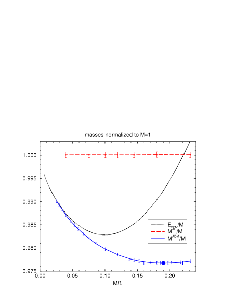
Figure 1: The ADM mass at infinity, the total 2PN energy, and the apparent horizon mass as a function of angular velocity. The minimum in $M^{ADM}_{\infty}$ at $M\Omega_{min}=0.19\pm 0.03$ is marked by a dot.

In Fig. 1 we show our results for the ADM mass $M^{ADM}_{\infty}$ at infinity and the apparent horizon mass

$$M^{AH}=\sqrt{A_{1}/16\pi}+\sqrt{A_{2}/16\pi}.$$ (6)

Here $A_{1}$ and $A_{2}$ are the areas of the two apparent horizons. In order to obtain coordinate independent results, all our graphs are plotted versus the angular velocity Tichy et al. (2003b)

$$\Omega=\frac{M^{ADM}_{\infty}-I_{K}({\alpha},S_{1})-I_{K}({\alpha},S_{2})}{2J^{ADM}_{\infty}},$$ (7)

instead of the coordinate separation $D$. For comparison, we also show the 2PN total energy Tichy et al. (2003a); Schäfer and Wex (1993)

$$E_{2PN} = M-\frac{\mu M}{2D}\Bigg{[}1+\Big{(}\frac{\mu}{M}-7\Big{)}\frac{M}{4D}$$ (8)

$$+ \!\!\!\Bigg{(}\frac{\mu^{2}}{M^{2}}+20\frac{\mu}{M}-9\Bigg{)}\frac{M^{2}}{8D^{2}}\Bigg{]}$$

versus the 2PN angular velocity Tichy et al. (2003a); Schäfer and Wex (1993)

$$\left(M\Omega_{2PN}\right)^{2} = \frac{64(D/M)^{3}}{(1+2D/M)^{6}}+\frac{\mu}{M}\left(\frac{M}{D}\right)^{4}$$ (9)

$$+ \!\!\!\left(\frac{\mu^{2}}{M^{2}}-\frac{5}{8}\frac{\mu}{M}\right)\left(\frac{M}{D}\right)^{5}.$$

Note that $\Omega_{2PN}$ in Eq. (9) is written such that $\Omega_{2PN}$ is exact up to all PN orders in the limit of $\mu/M\rightarrow 0$, while for $\mu/M>0$ Eq. (9) is accurate up to 2PN order. It should be kept in mind, however, that both, the resummation of Eq. (9), as well as the fact that $E_{2PN}$ is given as a function of $D$ instead of say $\Omega_{2PN}$, will change the $E_{2PN}$ versus $\Omega$ curve by PN terms higher than the $2PN$ terms included. This effect becomes noticeable around $M\Omega\gtrsim 0.1$, where these higher order terms become important.

The ADM mass $M^{ADM}_{\infty}$ approaches the PN result for large separations (i.e. small $\Omega$) as expected. Also, within our accuracy $M^{AH}$ is constant along the sequence. In previous works Cook (1994); Baumgarte (2000) this property was usually enforced in place of Eq. (1). It is interesting that the necessary conditions (3) and (4) for the existence of a helical Killing vector imply that $M^{ADM}_{A}=const$ and $M^{AH}=const$ are equivalent, and that in fact $2M^{ADM}_{A}=M=M^{AH}$. The ADM mass $M^{ADM}_{\infty}$ has a minimum at $M\Omega=M\Omega_{min}=0.19\pm 0.03$, which is usually interpreted as the innermost stable circular orbit (ISCO). This ISCO minimum occurs (within error bars) at the same angular velocity as the ones found by Cook Cook (1994) and Baumgarte Baumgarte (2000), using the effective potential method. Hence, results obtained using the assumption of a helical Killing vector are very similar to results found using the effective potential method. The reason for the relatively large error bar in $M\Omega_{min}$ comes from the fact that the minimum in $M^{ADM}_{\infty}$ is very shallow, so that the errors of order $0.03\%$ in our mass determination get amplified. Note, however, that our error estimate for $M\Omega_{min}$ is very conservative, as we have assumed that $M^{ADM}_{\infty}$ might randomly vary within $0.03\%$. If we instead assume that all values for $M^{ADM}_{\infty}$ are systematically too large or too small by $0.03\%$, the errorbar would be much smaller.

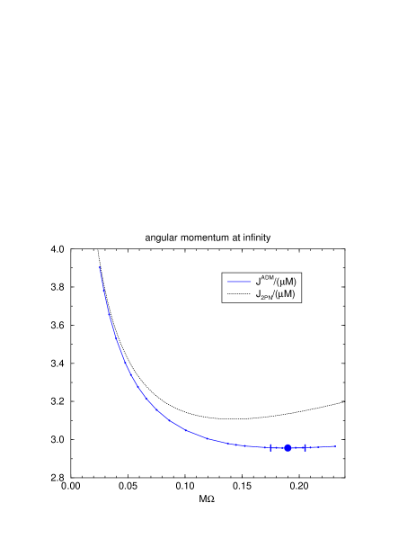
Figure 2: The ADM angular momentum at infinity and the 2PN angular momentum as a function of angular velocity. The minimum in $J^{ADM}_{\infty}$ at $M\Omega_{min}=0.190\pm 0.015$ is marked by a dot.

In Fig. 2 we show the ADM angular momentum $J^{ADM}_{\infty}$ as well as the 2PN angular momentum Tichy et al. (2003a); Schäfer and Wex (1993)

$$J_{2PN}^{2}=\mu^{2}MD\Bigg{[}1+4\frac{M}{D}+\frac{\left(74-43\frac{\mu}{M}\right)M^{2}}{8D^{2}}\Bigg{]}$$ (10)

versus $M\Omega$, which agree for small $\Omega$ as expected. As we can see, $J^{ADM}_{\infty}$ has its minimum at the same $\Omega$ as $M^{ADM}_{\infty}$. However, as $J^{ADM}_{\infty}$ varies more strongly than $M^{ADM}_{\infty}$ the minimum is less shallow, which allows us to locate it with better accuracy, with the result $M\Omega=M\Omega_{min}=0.190\pm 0.015$. Note that even though the error in $M\Omega_{min}$ is relatively large, we are able to determine all other quantities with an error of only about $0.03\%$.

Next, we list fits of several quantities along our numerically computed sequence. All fitted quantities are given as functions of the dimensionless orbital radius

$$x=\frac{D}{2M},$$ (11)

for the case of an equal mass binary. We find

$$\frac{m}{M} = \frac{1}{2}-\frac{0.0668549}{x}-\frac{0.0280090}{x^{\frac{3}{2}}}+\frac{0.0906937}{x^{2}}$$ (12)

$$-\frac{0.139304}{x^{\frac{5}{2}}}+\frac{0.0973014}{x^{3}}-\frac{0.0238708}{x^{\frac{7}{2}}},$$

$$\frac{P}{M} = \frac{1}{4{\sqrt{2x}}}-\frac{0.0123341}{x}+\frac{0.274250}{x^{\frac{3}{2}}}-\frac{0.317647}{x^{2}}$$ (13)

$$+\frac{0.554104}{x^{\frac{5}{2}}}-\frac{0.407033}{x^{3}}+\frac{0.101471}{x^{\frac{7}{2}}},$$

$$c = 1+\frac{0.0243978}{{\sqrt{x}}}-\frac{0.509913}{x}+\frac{0.629042}{x^{\frac{3}{2}}}$$ (14)

$$-\frac{1.00585}{x^{2}}+\frac{0.727406}{x^{\frac{5}{2}}}-\frac{0.177440}{x^{3}},$$

$$\frac{M^{ADM}_{\infty}}{M} = 1-\frac{1}{16x}+\frac{0.000684336}{x^{\frac{3}{2}}}+\frac{0.0499293}{x^{2}}$$ (15)

$$-\frac{0.00649266}{x^{\frac{5}{2}}}+\frac{0.0304472}{x^{3}}-\frac{0.0561704}{x^{\frac{7}{2}}}$$

$$+\frac{0.0209257}{x^{4}},$$

$$\frac{J^{ADM}_{\infty}}{\mu M} = 2x\frac{P}{\mu}=8x\frac{P}{M},$$ (16)

$$M\Omega = \frac{1}{2\,{\sqrt{2}}\,x^{\frac{3}{2}}}+\frac{0.0158006}{x^{2}}-\frac{0.347617}{x^{\frac{5}{2}}}+\frac{0.275492}{x^{3}}$$ (17)

$$-\frac{0.175001}{x^{\frac{7}{2}}}+\frac{0.0969903}{x^{4}}-\frac{0.0236081}{x^{\frac{9}{2}}}.$$

For the given expansions the fitting error is about $5\times 10^{-6}$. Our fits can be used to put two punctures into a quasi-circular orbit for any desired separation $D$. For the reader’s convenience we also list the results of these fits for a variety of separations in Tab. 1.

Table 1: Parameters for quasi-circular orbits of binary black hole puncture data. The errors in the quantities listed are of order $0.03\%$.

$D/2M$	$m/M$	$P/M$	$c$	$\frac{M^{ADM}_{\infty}}{M}$	$\frac{J^{ADM}_{\infty}}{\mu M}$	$M\Omega$
1.0300	0.43193	0.35879	0.69584	0.97681	2.9564	0.19008
1.0500	0.43318	0.35196	0.70109	0.97682	2.9564	0.18653
1.0750	0.43469	0.34380	0.70743	0.97683	2.9567	0.18223
1.1000	0.43613	0.33604	0.71354	0.97685	2.9571	0.17809
1.1250	0.43752	0.32865	0.71942	0.97689	2.9578	0.17409
1.1500	0.43885	0.32160	0.72509	0.97693	2.9587	0.17024
1.1750	0.44012	0.31488	0.73055	0.97698	2.9599	0.16652
1.2000	0.44135	0.30846	0.73581	0.97703	2.9612	0.16292
1.2250	0.44253	0.30232	0.74089	0.97710	2.9627	0.15945
1.2500	0.44366	0.29645	0.74580	0.97717	2.9645	0.15610
1.3000	0.44581	0.28543	0.75511	0.97732	2.9684	0.14972
1.3500	0.44780	0.27529	0.76380	0.97750	2.9731	0.14375
1.4000	0.44965	0.26594	0.77194	0.97769	2.9785	0.13815
1.4500	0.45138	0.25728	0.77957	0.97789	2.9844	0.13290
1.5000	0.45300	0.24924	0.78673	0.97811	2.9909	0.12797
1.6000	0.45593	0.23480	0.79981	0.97856	3.0055	0.11895
1.7000	0.45853	0.22219	0.81144	0.97903	3.0217	0.11092
1.8000	0.46084	0.21108	0.82184	0.97951	3.0395	0.10375
1.9000	0.46291	0.20123	0.83120	0.98000	3.0586	0.097299
2.0000	0.46477	0.19243	0.83964	0.98048	3.0788	0.091487
2.2500	0.46870	0.17406	0.85755	0.98164	3.1330	0.079215
2.5000	0.47185	0.15956	0.87192	0.98272	3.1911	0.069443
2.7500	0.47442	0.14780	0.88369	0.98372	3.2517	0.061518
3.0000	0.47656	0.13808	0.89350	0.98461	3.3138	0.054988
3.5000	0.47992	0.12287	0.90891	0.98619	3.4404	0.044923
4.0000	0.48243	0.11148	0.92044	0.98750	3.5674	0.037589
4.5000	0.48439	0.10259	0.92940	0.98859	3.6934	0.032052
5.0000	0.48595	0.095433	0.93655	0.98952	3.8173	0.027753
6.0000	0.48830	0.084541	0.94726	0.99099	4.0580	0.021565
7.0000	0.48997	0.076578	0.95491	0.99211	4.2884	0.017378
8.0000	0.49123	0.070451	0.96064	0.99299	4.5089	0.014390
9.0000	0.49220	0.065559	0.96511	0.99369	4.7203	0.012171
10.000	0.49299	0.061542	0.96868	0.99427	4.9233	0.010468

III Discussion

We have constructed a sequence of binary black hole puncture data by using the necessary helical Killing vector conditions (3) and (4) and by assuming that $M^{ADM}_{A}$ is constant along the sequence. The numerical results are obtained for equal mass binaries without spin, but our approach can also be applied in the general case. Our sequence is close to quasi-equilibrium in the following sense. The time derivative of the trace of the extrinsic curvature is zero, due to the choice of a maximal slicing lapse. The conformal metric and conformal factor evolve on a timescale long compared to the orbital timescale, if we also compute a shift as in Tichy et al. (2003b), which removes the longitudinal piece of the time derivative of the conformal metric. With this gauge choice the time derivative of the tracefree part of the extrinsic curvature is also reduced, but it still evolves on the orbital timescale.

We find that the apparent horizon mass $M_{AH}$ is constant along the sequence up to our numerical accuracy, and that $M_{AH}=M^{ADM}_{1}+M^{ADM}_{2}$. Furthermore, the ISCO minimum in both $M^{ADM}_{\infty}$ and $J^{ADM}_{\infty}$ occurs at the same $\Omega$, but the error bars on the minimum on in $J^{ADM}_{\infty}$ are tighter. Previous results for the ISCO Cook (1994); Baumgarte (2000) agree with our result within error bars, but our ISCO is at a somewhat higher $\Omega$.

Baker Baker (2002) has constructed a puncture sequence using an effective potential method and the assumption that $M^{ADM}_{A}$ is constant along the sequence. His results are similar to ours. Yet even though he has used fixed mesh refinement for computational efficiency, his values seem to be less accurate. In Baker (2002), the outer boundary was put at large distances in order to compute $M^{ADM}_{\infty}$ with sufficient accuracy, but based on our numerical results the resolution near the black holes appears to be rather low.

The parameters for quasi-circular orbits in Tab. 1 can be compared with the data for the effective potential method in the form given in Baker et al. (2002b), which provides a sequence translated from Misner type black hole excision data of Cook Cook et al. (1993); Cook (1994) to puncture data assuming that both types of data are numerically close. Our data is likely to be more accurate than effective potential method data since we do not have to find turning points in potentially very flat ADM mass curves to determine if an orbit is circular. Also, our masses are computed with much higher accuracy than in Baker et al. (2002b). For example, for $D/2=1.7846M=1.8490M^{ADM}_{\infty}$ there is a discrepancy of $1\%$. Yet part of the difference may be due to the fact that we use the helical Killing vector conditions (3) and (4) instead of effective potential method to find quasi-circular orbits. The fact that we have kept $M^{ADM}_{A}$ constant along the sequence and not $M_{AH}$ as in Cook (1994) and Baumgarte (2000) should not play a role as both seem to be equivalent along our sequence.

Finally, we want to mention that G. Cook has informed us that M. Hannam has just completed his Ph.D. thesis which includes the discussion of a puncture sequence that shares some of the features of our work.

Appendix A Computing masses at infinity on a finite grid

In order to implement Eqs. (3) and (4), we have to determine the masses with sufficient accuracy. In particular, we have to compute the ADM mass at infinity to a rather high accuracy of about $10^{-4}M$. Since in the case of punctures Brandt and Brügmann (1997) the 3-metric is conformally flat with a conformal factor

$$\phi=1+\frac{m_{1}}{2r_{1}}+\frac{m_{2}}{2r_{2}}+u,$$ (18)

the ADM mass at infinity is given by

$$M^{ADM}_{\infty}=-\frac{1}{2\pi}\int\nabla^{2}\phi\ dV=m_{1}+m_{2}-\frac{1}{2\pi}\int\nabla^{2}u\ dV,$$ (19)

Here $u$ has to be determined from an elliptic equation of the form Tichy et al. (2003b); Brandt and Brügmann (1997)

$$\nabla^{2}u=f(u),$$ (20)

with boundary condition

$$\lim_{r\rightarrow\infty}u=0.$$ (21)

As our numerical grid does not extend all the way to infinity, we cannot directly compute the volume integral in Eq. (19). Using a coordinate transformation in the radial direction, e.g. of the “FishEye” type Baker et al. (2000), helps but does not necessarily give sufficiently accurate results because of finite difference errors in the far region. Instead, the last term of Eq. (19) can be approximated by the integral

$$I_{1}=\int_{0}^{R_{1}}f(u)\ dV$$ (22)

over the numerical grid up to the outer boundary denoted by $R_{1}$. Then

$$\int\nabla^{2}u\ dV=I_{1}+O(1/R_{1}),$$ (23)

where $O(1/R_{1})$ is the error due to truncating the integral at a finite radius $R_{1}$. This error is often too large as it falls off only like $1/R_{1}$ (see the curves labeled “grid only” in Fig. 3). For this reason we want to improve the approximation by integrating over a region larger than the grid, which extends to at least $R_{2}\sim R_{1}^{2}$, so that the error goes down by one additional power in $1/R_{1}$. I.e. we want to approximate the volume integral by

$$\int\nabla^{2}u\ dV=I_{1}+I_{2}+O(1/R_{2})=I_{1}+I_{2}+O(1/R_{1}^{2}),$$ (24)

where

$$I_{2}=\int_{R_{1}}^{R_{2}}f(u)\ dV.$$ (25)

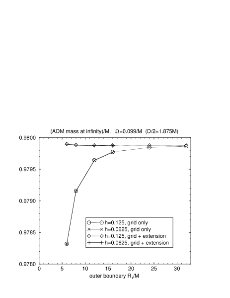
Figure 3: $M^{ADM}_{\infty}$ computed using integral (23) over the numerical grid only, compared with $M^{ADM}_{\infty}$ computed using the extended volume integral (31) with $R_{2}=10R_{1}^{2}/M$ for two different resolutions $h$. The extended integral (31) gives much more accurate results.

The problem with this approach is that we have computed $u$ only on the numerical grid, so that we have to somehow approximate $u$ outside the grid. This can be achieved by noting that because of boundary condition (21)

$$u=\frac{a_{1}}{r}+O(1/r^{2})$$ (26)

for large distances $r$, so that

$$I_{1}=\int_{0}^{R_{1}}\nabla^{2}u\ dV=\oint_{R_{1}}\nabla_{i}u\ dS^{i}=-4\pi a_{1}+O(1/R_{1}).$$ (27)

Hence outside the numerical grid $u$ can be approximated by

$$u=-\frac{1}{4\pi}\frac{I_{1}}{r}+O\left(\frac{1}{rR_{1}}\right)+O\left(\frac{1}{r^{2}}\right)$$ (28)

where $I_{1}$ is computed only on the grid. Also, note that for large $r$

$$f(u)\sim\frac{1}{r^{4}},$$ (29)

otherwise the ADM mass integral in Eq. (19) would be infinite. Thus, if we insert Eq. (28) into Eq. (25) and also take into account the falloff behavior (29) of $f(u)$ we arrive at

$$I_{2}=\int_{R_{1}}^{R_{2}}f\left(-\frac{1}{4\pi}\frac{I_{1}}{r}\right)\ dV+O\left(\frac{1}{R_{1}^{2}}\right).$$ (30)

Combining Eqs. (24) and (30) we arrive at the final result

$$\int\nabla^{2}u\ dV=I_{1}+\int_{R_{1}}^{R_{2}}f\left(-\frac{1}{4\pi}\frac{I_{1}}{r}\right)\ dV+O\left(\frac{1}{R_{1}^{2}}\right),$$ (31)

which depends only on $I_{1}$ computed from $u$ on the numerical grid and a volume integral outside the grid over the known function $f$.

We have applied the method described in the previous paragraph to both the ADM and Komar mass integrals at infinity, as both can be expressed as volume integrals. Fig. 3 shows $M^{ADM}_{\infty}$ computed using the extended volume integral (31) as well as the result if we integrate only over the grid using Eq. (23). The extended volume integral result is clearly more accurate, say for $R_{1}=12M$, which we have used to obtain our sequence.

References

- Schutz (1999) B. Schutz, Class. Quantum Grav. 16, A131 (1999).
- Cook (2000) G. B. Cook, Living Reviews in Relativity 2000, 5 (2000).
- Tichy et al. (2003a) W. Tichy, B. Brügmann, M. Campanelli, and P. Diener, Phys. Rev. D 67, 064008 (2003a), gr-qc/0207011.
- Cook (1994) G. B. Cook, Phys. Rev. D 50, 5025 (1994).
- Gourgoulhon et al. (2001) E. Gourgoulhon, P. Grandclement, and S. Bonazzola, Phys. Rev. D 65, 044020 (2001), eprint gr-qc/0106015.
- Tichy et al. (2003b) W. Tichy, B. Brügmann, and P. Laguna (2003b), gr-qc/0306020.
- Brandt and Brügmann (1997) S. Brandt and B. Brügmann, Phys. Rev. Lett. 78, 3606 (1997).
- Brügmann (1999) B. Brügmann, Int. J. Mod. Phys. D 8, 85 (1999).
- Alcubierre et al. (2001) M. Alcubierre, W. Benger, B. Brügmann, G. Lanfermann, L. Nerger, E. Seidel, and R. Takahashi, Phys. Rev. Lett. 87, 271103 (2001), eprint gr-qc/0012079.
- Alcubierre et al. (2003) M. Alcubierre, B. Brügmann, P. Diener, M. Koppitz, D. Pollney, E. Seidel, and R. Takahashi, Phys. Rev. D 67, 084023 (2003), eprint gr-qc/0206072.
- Baker et al. (2000) J. Baker, B. Brügmann, M. Campanelli, and C. O. Lousto, Class. Quantum Grav. 17, L149 (2000).
- Baker et al. (2002a) J. Baker, M. Campanelli, and C. O. Lousto, Phys. Rev. D65, 044001 (2002a), eprint [http://arXiv.org/abs]gr-qc/0104063.
- Baker et al. (2001) J. Baker, B. Brügmann, M. Campanelli, C. O. Lousto, and R. Takahashi, Phys. Rev. Lett. 87, 121103 (2001), eprint [http://arXiv.org/abs]gr-qc/0102037.
- Baker et al. (2002b) J. Baker, M. Campanelli, C. O. Lousto, and R. Takahashi, Phys. Rev. D65, 124012 (2002b), eprint [http://arXiv.org/abs]astro-ph/0202469.
- Baumgarte (2000) T. W. Baumgarte, Phys. Rev. D 62, 024018 (2000), eprint gr-qc/0004050.
- Baker (2002) B. D. Baker (2002), eprint [http://arXiv.org/abs]gr-qc/0205082.
- Blackburn and Detweiler (1992) J. K. Blackburn and S. Detweiler, Phys. Rev. D 46, 2318 (1992).
- Schäfer and Wex (1993) G. Schäfer and N. Wex, Physics Lett. A 174, 196 (1993).
- Cook et al. (1993) G. B. Cook, M. W. Choptuik, M. R. Dubal, S. Klasky, R. A. Matzner, and S. R. Olivera, Phys. Rev. D 47, 1471 (1993).