Abstract. Cosmological equations for homogeneous isotropic models filled by scalar fields and ultrarelativistic matter are investigated in the framework of gauge theories of gravity. Regular inflationary cosmological models of flat, closed and open type with dominating ultrarelativistic matter at a bounce are discussed. It is shown that essential part of inflationary cosmological models has bouncing character.
PACS numbers: 0420J, 0450, 1115, 9880
KEYWORDS: Cosmological singularity, bounce, inflation, gauge theories of gravity

1 Introduction

It is known that inflationary scenario plays the important role in the early Universe theory and allows to resolve a number of problems of standard Friedmann cosmology [1, 2]. Most inflationary models built in the frame of general relativity theory (GR) are singular and limited in the time in the past. In the case of flat and open models such situation is inevitable [3], and the quantum gravity era cannot be avoided in the past. At the same time regular inflationary bouncing solutions exist in GR for closed models filled by massive or nonlinear scalar fields and usual matter [5-12]. Because limiting (maximum) energy density and limiting temperature at a bounce in such models can be essentially less than the Planckian ones, classical description of gravitational field in these models is possible and quantum gravitational effects are negligible. Note that regular inflationary solutions for closed models in GR are unstable at compression stage, and small variations of gravitational and scalar fields at compression lead to singularity because of the divergence of the time derivative of scalar field $\dot{\phi}$. As result the energy density $\rho_{\phi}=\frac{1}{2}\dot{\phi}^{2}+V(\phi)$ and the pressure $p=\frac{1}{2}\dot{\phi}^{2}-V(\phi)$ ($V$ is a scalar field potential) of scalar field at compression stage near singularity are connected in the following way $p_{\phi}\approx\rho_{\phi}$ [7]. In the case of regular bouncing solutions the scalar field potential has to be dominating at a bounce, so in the case of models including scalar field $\phi$ and ultrarelativistic matter with the energy density $\rho_{r}$ the following condition at a bounce must be valid

$$V-\dot{\phi}^{2}-\rho_{r}>0.$$ (1)

The relation (1) means that the greatest part of energy density at the end of cosmological compression has to be determined by scalar fields. Because there are not physical reasons ensuring the realization of condition (1), regular inflationary solutions in GR cannot be considered as a base to build regular inflationary cosmology.

Different situation takes place in gauge theories of gravitation (GTG) - Poincare GTG, metric-affine GTG. Note that GTG are natural generalization of GR by applying the local gauge invariance principle to gravitational interaction (see review [14]). As it was shown in a number of our papers [15-20,12], the GTG possess important regularizing properties. By satisfying the correspondence principle with GR in the case of usual gravitating systems with rather small energy densities and pressures, GTG can lead to essentially different physical conclusions in the case of gravitating systems at extreme conditions with extremely high energy densities and pressures [15, 17]. In particular, gravitating vacuum with sufficiently high energy density $\rho_{v}>0$ and pressure $p_{v}=-\rho_{v}$ can lead to the vacuum gravitational repulsion effect and to a bounce in closed, open and flat models, that allows to build regular inflationary cosmological models [16, 10, 12]. Some particular regular inflationary cosmological solutions for closed models with scalar fields were discussed in Refs.[21, 11, 12]. The present paper is devoted to study the problem what place take regular inflationary cosmological models in GTG.

2 Generalized cosmological Friedmann equations in GTG

Homogeneous isotropic models in GTG are described by the following generalized cosmological Friedmann equations (GCFE)

$$\frac{k}{R^{2}}+\left\{\frac{d}{dt}\ln\left[R\sqrt{\left|1-\beta\left(\rho-3p\right)\right|}\,\right]\right\}^{2}=\frac{8\pi}{3M_{p}^{2}}\,\frac{\rho-\frac{\beta}{4}\left(\rho-3p\right)^{2}}{1-\beta\left(\rho-3p\right)}\,,$$ (2)

$$\frac{\left[\dot{R}+R\left(\ln\sqrt{\left|1-\beta\left(\rho-3p\right)\right|}\,\right)^{\cdot}\right]^{\cdot}}{R}=-\frac{4\pi}{3M_{p}^{2}}\,\frac{\rho+3p+\frac{\beta}{2}\left(\rho-3p\right)^{2}}{1-\beta\left(\rho-3p\right)}\,,$$ (3)

where $R(t)$ is the scale factor of Robertson-Walker metrics, $k=+1,0,-1$ for closed, flat, open models respectively, $\rho$ is energy density, $p$ is pressure, $\beta$ is indefinite parameter with inverse dimension of energy density, $M_{p}$ is Planckian mass. (The system of units with $\hbar=c=1$ is used). At first the GCFE were deduced in Poincare GTG [15], and later it was shown that Eqs.(2)-(3) take place also in metric-affine GTG [22, 23]. From Eqs. (2)-(3) follows the conservation law in usual form

$$\dot{\rho}+3H\left(\rho+p\right)=0,$$ (4)

where $H=\frac{\dot{R}}{R}$ is the Hubble parameter. Besides cosmological equations (2)-(3) gravitational equations of GTG lead to the following relation for torsion function $S$ and nonmetricity function $Q$

$$S-\frac{1}{4}Q=-\frac{1}{4}\,\frac{d}{dt}\ln\left|1-\beta(\rho-3p)\right|.$$ (5)

In Poincare GTG $Q=0$ and Eq. (5) determines the torsion function. In metric-affine GTG there are three kinds of models [23]: in the Riemann-Cartan space-time ($Q=0$), in the Weyl space-time ($S=0$), in the Weyl-Cartan space-time ($S\neq 0$, $Q\neq 0$, the function S is proportional to the function $Q$). The value of $|\beta|^{-1}$ determines the scale of extremely high energy densities. The GCFE (2)-(3) coincide practically with Friedmann cosmological equations of GR if the energy density is small $\left|\beta(\rho-3p)\right|\ll 1$. The difference between GR and GTG can be essential at extremely high energy densities $\left|\beta(\rho-3p)\right|\gtrsim 1$. In the case of gravitating vacuum with constant energy density $\rho_{v}=\mathrm{const}>0$ the GCFE (2)–(3) are reduced to Friedmann cosmological equations of GR and $S=Q=0$, this means that de Sitter solutions for metrics with vanishing torsion and nonmetricity are exact solutions of GTG [24, 25] and hence inflationary models can be built in the frame of GTG.

In order to analyze inflationary cosmological models in GTG let us consider systems including scalar field minimally coupled with gravitation and usual matter in the form of ultrarelativistic matter. This assumption is available by analysis of the hot Universe models in the beginning of cosmological expansion. In the case of other form of gravitating matter our consideration would be more complicated. If the interaction between scalar field and ultrarelativistic matter is negligible, the energy density $\rho$ and pressure $p$ take the form

$$\rho=\frac{1}{2}\dot{\phi}^{2}+V(\phi)+\rho_{r},\qquad p=\frac{1}{2}\dot{\phi}^{2}-V(\phi)+\frac{1}{3}\rho_{r},$$ (6)

and the conservation law (4) leads to the scalar field equation

$$\ddot{\phi}+3H\dot{\phi}=-V^{\prime}\qquad\left(V^{\prime}=\frac{dV}{d\phi}\right)$$ (7)

and the conservation law for matter, which in our case has the following integral ${\rho_{r}R^{4}={\rm const}}$. By using Eqs. (6)-(7) the GCFE (2)-(3) can be written in the following form

$$\frac{k}{R^{2}}Z^{2}+\left\{H\left[1-2\beta(2V+\dot{\phi}^{2})\right]-3\beta V^{\prime}\dot{\phi}\right\}^{2}$$

$$\phantom{+H\left[1-2\beta(2V+\dot{\phi}^{2})\right]}=\frac{8\pi}{3M_{p}^{2}}\,\left[\rho_{r}+\frac{1}{2}\dot{\phi}^{2}+V-\frac{1}{4}\beta\left(4V-\dot{\phi}^{2}\right)^{2}\right]Z,$$ (8)

$$\dot{H}\left[1-2\beta(2V+\dot{\phi}^{2})\right]Z+H^{2}\left\{\left[1-4\beta(V-4\dot{\phi}^{2})\right]Z-18\beta^{2}\dot{\phi}^{4}\right\}$$

$$\phantom{H}+12\beta H\dot{\phi}V^{\prime}\left[1-2\beta(2V+\dot{\phi}^{2})\right]-3\beta\left[(V^{\prime\prime}\dot{\phi}^{2}-V^{\prime}{}^{2})Z+6\beta\dot{\phi}^{2}V^{\prime}{}^{2}\right]$$

$$\phantom{\dot{H}\left[1-2\beta(2V+\dot{\phi}^{2})\right]Z}=\frac{8\pi}{3M_{p}^{2}}\,\left[V-\dot{\phi}^{2}-\rho_{r}-\frac{1}{4}\beta(4V-\dot{\phi}^{2})^{2}\right]Z,$$ (9)

where $Z=1-\beta(4V-\dot{\phi}^{2})$, $\displaystyle V^{\prime}=\frac{dV}{d\phi}$, $\displaystyle V^{\prime\prime}=\frac{d^{2}V}{d\phi^{2}}$. Relation (5) takes the form

$$S-\frac{1}{4}Q=\frac{3\beta}{2}\,\frac{\left(H\dot{\phi}+V^{\prime}\right)\dot{\phi}}{1-\beta\left(4V-\dot{\phi}^{2}\right)}.$$ (10)

Unlike GR the cosmological equation (8) leads to essential restrictions on admissible values of scalar field and permits to exclude the divergence of derivative $\dot{\phi}$ for any finite value of $\phi$, if $\beta<0$. Imposing $\beta<0$, we obtain from Eq. (8) in the case $k=0,+1$

$$Z\geq 0\qquad\text{or}\qquad\dot{\phi}^{2}\leq 4V+|\beta|^{-1}.$$ (11)

Inequality (11) is valid also for open models discussed in Sec. 3. The region $\Sigma$ of admissible values of scalar field on the plane $P$ with the axis ($\phi$, $\dot{\phi}$) determined by (11) is limited by two bounds $L_{\pm}$

$$\dot{\phi}=\pm\left(4V+|\beta|^{-1}\right)^{\frac{1}{2}}.$$ (12)

From Eq. (8) the Hubble parameter on the bounds $L_{\pm}$ is equal to

$$H=\frac{3\beta V^{\prime}\dot{\phi}}{1-2\beta(2V+\dot{\phi}^{2})}.$$ (13)

According to (13) the right-hand part of Eq. (10) is equal to $\frac{1}{2}H$ on the bounds $L_{\pm}$. This means that the torsion (nonmetricity) will be regular, if the Hubble parameter and scalar field are regular. In connection with this our main attention in Sec. 3 will be turned to study properties of solutions of GCFE (8)-(9). In accordance with (11) energy density $\rho_{\phi}$ and pressure $p_{\phi}$ of scalar field satisfy the condition $p_{\phi}\leq\frac{1}{3}(\rho_{\phi}+|\beta|^{-1})$. Unlike GR the equation of state for scalar field $p_{\phi}\approx\rho_{\phi}$ is not valid at any stage of models evolution in GTG.

3 Regular inflationary models in GTG

Let us consider the most important general properties of cosmological solutions of GCFE (8)-(9). At first, note by given initial conditions for scalar field ($\phi$,$\dot{\phi}$) and values of $R$ and $\rho_{r}$ there are two different solutions corresponding to two values of the Hubble parameter following from Eq. (8):

$$H_{\pm}=\frac{3\beta V^{\prime}\dot{\phi}\pm\sqrt{D}}{1-2\beta(2V+\dot{\phi}^{2})},$$

where

$$D=\frac{8\pi}{3M_{p}^{2}}\,\left[\rho_{r}+\frac{1}{2}\dot{\phi}^{2}+V-\frac{1}{4}\beta\left(4V-\dot{\phi}^{2}\right)^{2}\right]Z-\frac{k}{R^{2}}\,Z^{2}\geq 0$$

Unlike GR, the values of $H_{+}$ and $H_{-}$ in GTG are sign-variable and, hence, both solutions corresponding to $H_{+}$ and $H_{-}$ can describe the expansion as well as the compression in dependence on their sign. Below we will call solutions of GCFE corresponding to $H_{+}$ and $H_{-}$ as $H_{+}$-solutions and $H_{-}$-solutions respectively. In points of bounds $L_{\pm}$ we have $D=0$, $H_{+}=H_{-}$ and the Hubble parameter is determined by (13). The bounds $L_{\pm}$ are particular curves for GCFE. If $Z=0$, Eqs. (8)–(9) are satisfied, and because the bounds $L_{\pm}$ are not limited for applying potentials $V(\phi)$ and tend to infinity under $|\phi|\to\infty$, corresponding solutions of GCFE are singular.

In order to study the behaviour of cosmological models at the beginning of cosmological expansion, let us analyze extreme points for the scale factor $R(t)$: $R_{0}=R(0)$, $H_{0}=H(0)=0$. Denoting values of quantities at $t=0$ by means of index ”0”, we obtain from (8)-(9):

$$\frac{k}{R_{0}^{2}}Z_{0}^{2}+9\beta^{2}V^{\prime}{}_{0}^{2}\dot{\phi}_{0}^{2}=\frac{8\pi}{3M_{p}^{2}}\,\left[\rho_{r0}+\frac{1}{2}\dot{\phi_{0}}^{2}+V_{0}-\frac{1}{4}\beta\left(4V_{0}-\dot{\phi}_{0}^{2}\right)^{2}\right]Z_{0},$$ (14)

$$\dot{H}_{0}=\left\{\frac{8\pi}{3M_{p}^{2}}\,\left[V_{0}-\dot{\phi}_{0}^{2}-\rho_{r0}-\frac{1}{4}\beta(4V_{0}-\dot{\phi}_{0}^{2})^{2}\right]Z_{0}\right.$$

$$\left.\phantom{H_{0}=}+3\beta\left[(V^{\prime\prime}{}_{0}\dot{\phi}_{0}^{2}-V^{\prime}{}_{0}^{2})Z_{0}+6\beta\dot{\phi}_{0}^{2}V^{\prime}{}_{0}^{2}\right]\right\}\left[1-2\beta(2V_{0}+\dot{\phi}_{0}^{2})\right]^{-1}Z_{0}^{-1},$$ (15)

where $Z_{0}=1-\beta(4V_{0}-\dot{\phi}_{0}^{2})$. A bounce point is described by Eq. (14), if the value of $\dot{H}_{0}$ is positive. By giving concrete form of potential $V$ and choosing values of $R_{0}$, $\phi_{0}$, $\dot{\phi}_{0}$ and $\rho_{r0}$ at a bounce, we can obtain numerically particular bouncing solutions of GCFE for various values of parameter $\beta$.

The analysis of GCFE shows, that the properties of cosmological solutions depend essentially on the parameter $\beta$, i.e. on the scale of extremely high energy densities. From physical point of view interesting results can be obtained, if the value of $|\beta|^{-1}$ is much less than the Planckian energy density [12], i.e. in the case of large in module values of parameter $\beta$ (by imposing $M_{p}=1$). In order to investigate cosmological solutions at the beginning of cosmological expansion in this case, let us consider the GCFE by supposing that

$$\left|\beta\left(4V-\dot{\phi}^{2}\right)\right|\gg 1,\qquad\rho_{r}+\frac{1}{2}\dot{\phi}^{2}+V\ll\left|\beta\right|\left(4V-\dot{\phi}^{2}\right)^{2}.$$ (16)

Note that the second condition (16) does not exclude that ultrarelativistic matter energy density can dominate at a bounce $\rho_{r}\gg V+\frac{1}{2}\dot{\phi}^{2}$ [12]. We obtain:

$$\frac{k}{R^{2}}+\frac{\left[2H\left(2V+\dot{\phi}^{2}\right)+3V^{\prime}\dot{\phi}\right]^{2}}{\left(4V-\dot{\phi}^{2}\right)^{2}}=\frac{2\pi}{3M_{p}^{2}}\left(4V-\dot{\phi}^{2}\right),$$ (17)

$$\dot{H}\left(2V+\dot{\phi}^{2}\right)\left(4V-\dot{\phi}^{2}\right)+H^{2}\left(8V^{2}-34V\dot{\phi}^{2}-\dot{\phi}^{4}\right)-12HV^{\prime}\dot{\phi}\left(2V+\dot{\phi}^{2}\right)\\ +\frac{3}{2}\left(V^{\prime\prime}\dot{\phi}^{2}-V^{\prime 2}\right)\left(4V-\dot{\phi}^{2}\right)-9V^{\prime 2}\dot{\phi}^{2}=\frac{\pi}{3M_{p}^{2}}\left(4V-\dot{\phi}^{2}\right)^{3}.$$ (18)

Eqs. (17)-(18) do not include radiation energy density, which does not have influence on the dynamics of inflationary models in the case under consideration (although, as it was noted above, the contribution of ultrarelativistic matter to energy density can be essentially greater in comparison with scalar field), moreover Eqs. (17)-(18) do not contain the parameter $\beta$. According to Eq. (17) the Hubble parameter in considered approximation is equal to

$$H_{\pm}=\frac{\displaystyle-3V^{\prime}\dot{\phi}\pm\left|4V-\dot{\phi}^{2}\right|\,\sqrt{\frac{2\pi}{3M_{p}^{2}}\left(4V-\dot{\phi}^{2}\right)-\frac{k}{R^{2}}}}{\displaystyle 2\left(2V+\dot{\phi}^{2}\right)}\,,$$

and extreme points of the scale factor are determined by the following condition

$$\frac{k}{R_{0}^{2}}+9\left(\frac{V_{0}^{\prime}\dot{\phi}_{0}}{4V_{0}-\dot{\phi}^{2}_{0}}\right)^{2}=\frac{2\pi}{3M_{p}^{2}}\left(4V_{0}-\dot{\phi}^{2}_{0}\right).$$ (19)

From Eq. (18) the time derivative of the Hubble parameter at extreme points is

$$\dot{H}_{0}=\left[\frac{\pi}{3M_{p}^{2}}\,\left(4V_{0}-\dot{\phi}_{0}^{2}\right)^{2}+\frac{3}{2}\left(V_{0}^{\prime 2}-V_{0}^{\prime\prime}\dot{\phi}_{0}^{2}\right)+9V_{0}^{\prime 2}\dot{\phi}_{0}^{2}\left(4V_{0}-\dot{\phi}_{0}^{2}\right)^{-1}\right]\left(2V_{0}+\dot{\phi}_{0}^{2}\right)^{-1}.$$ (20)

Obviously Eq. (19)-(20) correspond to (14)-(15) in considered approximation.

Now let us consider flat models, for which Eq. (19) can be written in the following form

$$4V_{0}-\dot{\phi}_{0}^{2}=3\left(\frac{M_{p}^{2}}{2\pi}\,{V_{0}^{\prime}}^{2}\,\dot{\phi}_{0}^{2}\right)^{\frac{1}{3}}.$$ (21)

Solutions of Eq. (21) are in physical region $\Sigma$ on the plane $P$ determined in considered approximation according to (11) by the following inequality $4V-\dot{\phi}^{2}>0$ (the neighbourhood of origin of coordinates on the plane $P$ is not considered in our approximation). Eq.(21) has as solutions two curves $B_{1}$ and $B_{2}$ on the plane $P$, which are situated near bounds $L_{+}$ and $L_{-}$ respectively. Because of (21) the bounce condition $\dot{H}_{0}>0$ can be written in the form

$$\frac{2\pi}{3M_{p}^{2}}\,\left(4V_{0}-\dot{\phi}_{0}^{2}\right)^{2}+V_{0}^{\prime 2}-V_{0}^{\prime\prime}\dot{\phi}_{0}^{2}>0\quad\text{or}\quad 6\left(\frac{\pi}{4M_{p}^{2}}\right)^{\frac{1}{3}}\left(V^{\prime}_{0}\,\dot{\phi}_{0}\right)^{\frac{4}{3}}+V_{0}^{\prime 2}-V_{0}^{\prime\prime}\dot{\phi}_{0}^{2}>0.$$ (22)

If the condition (22) is satisfied on the curves $B_{1,2}$, the bounce will take place for corresponding solutions in points of these curves, which can be called ”bounce curves”. Note that bounce curves exist in the case of various scalar field potentials applying in inflationary cosmology, in particular, in the case of power potentials $V=\alpha\phi^{2n}$ ($\alpha=\mathrm{const}>0$ and $n$ is integer positive number). Each of two curves $B_{1,2}$ contains two parts corresponding to vanishing of $H_{+}$ or $H_{-}$ and denoting by ($B_{1+}$, $B_{2+}$) and ($B_{1-}$, $B_{2-}$) respectively. If $V^{\prime}$ is positive (negative) in quadrants 1 and 4 (2 and 3) on the plane $P$, the bounce will take place in points of bounce curves $B_{1+}$ and $B_{2+}$ ($B_{1-}$ and $B_{2-}$) in quadrants 1 and 3 (2 and 4) for $H_{+}$-solutions ($H_{-}$-solutions) (see Fig. 1).

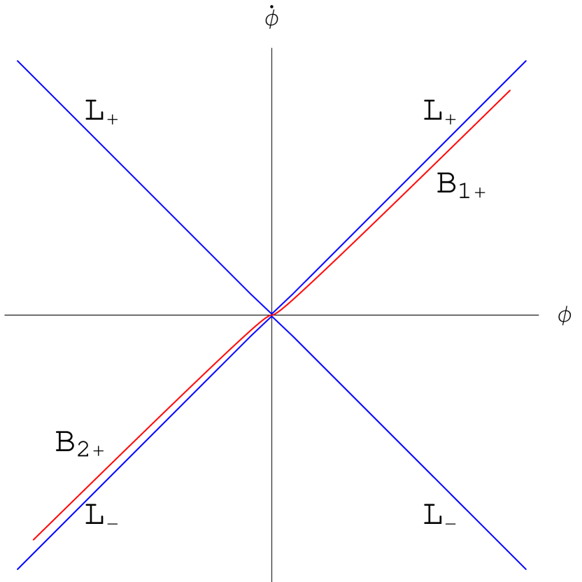
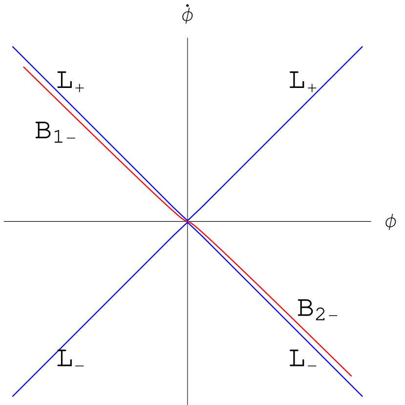
Figure 1: Bounce curves for $H_{+}$-solutions and $H_{-}$-solutions in the case of potential $V=\frac{1}{2}m^{2}\phi^{2}$.

As result practically all phase trajectories for $H_{+}$–solutions ($H_{-}$–solutions) reaching bounce curves $B_{1+}$ and $B_{2+}$ ($B_{1-}$ and $B_{2-}$) correspond to bouncing solutions. To obtain regular bouncing solutions we have to take into account that bounds $L_{\pm}$ defined by relation $Z=0$ and Eq.(13) correspond to particular solutions of GCFE ($L_{\pm}$–solutions), in points of which $H_{-}$–solutions reach the bounds and $H_{+}$–solutions originate from them. As result the regular transition from $H_{-}$–solutions to $H_{+}$–solutions is possible on bounds $L_{\pm}$, in particular, in the form of their glueing. In consequence of this each solution containing as parts $H_{-}$-solution and $H_{+}$-solution describes regular inflationary model, and a bounce takes place by intersection of phase trajectory with corresponding bounce curve. However, singular solutions exist also. As it was noted above in the case of various potentials applying in inflationary cosmology (in particular, power potentials) the curves $L_{\pm}$ are not limited on the plane P and tend to infinity; the scalar field satisfying the following equation on bounds $\ddot{\phi}=2V^{\prime}$ diverges in the past and in the future, and hence particular $L_{\pm}$ -solutions are singular. As result any solution containing $H_{+}$-solution (or $H_{-}$-solution) glueed with particular $L_{\pm}$-solutions is singular in the past (or in the future). Note the number of such singular solutions is much less than the number of regular solutions, namely to one singular solution correspond infinite number of regular solutions obtaining by glueing of noted above singular solution with $H_{-}$-solution (or $H_{+}$-solution) in different points of $L_{\pm}$-curve and excluding then divergent part of $L_{\pm}$ -solution.

In the case of open and closed models Eq. (19) determines 1-parametric family of bounce curves with parameter $R_{0}$. Bounce curves of closed models are situated on the plane $P$ in region between two bounce curves $B_{1}$ and $B_{2}$ of flat models, and in the case of open models bounce curves are situated in two regions between the curves: $L_{+}$ and $B_{1}$, $L_{-}$ and $B_{2}$. Because the behaviour of bounce curves for open models is like to that for flat models, the situation concerning bouncing inflationary solutions in the case of open models is the same as described above situation for flat models. Unlike flat and open models, for which $H_{+}=H_{-}$ only in points of bounds $L_{\pm}$ and regular inflationary models can be built if $H_{+}$– and $H_{-}$–solutions reach bounds$L_{\pm}$, in the case of closed models the regular transition from $H_{-}$-solution to $H_{+}$-solution is possible without reaching the bounds $L_{\pm}$. It is because by certain value of $R$ we have $H_{+}=H_{-}$ in the case if $Z\neq 0$. Similar regular inflationary solution was considered in Ref.[12]. Note that bouncing solutions exist not only in classical region, where scalar field potential and kinetic energy density of scalar field go not exceed the Planckian energy density, but also in regions, where classical restrictions on scalar fields are not fulfilled and according to accepted opinion quantum gravitational effects can be essential.

In general case, when approximation (16) is not valid, bounce curves of cosmological models determined by Eq.(14) depend on parameter $\beta$ . By certain value of $\beta$ we have 1-parametric family of bounce curves with parameter $\rho_{r0}$ for flat models, and we have 2-parametric families of bounce curves for closed and open models with parameters $R_{0}$ and $\rho_{r0}$. According to Eqs. (14)–(15) the bounce condition $\dot{H}_{0}>0$ leads to the following relation

$$\frac{8\pi}{3M_{p}^{2}}\,\left[V_{0}+\frac{1}{3}\rho_{r0}-\frac{1}{4}\beta\left(4V_{0}-\dot{\phi}_{0}^{2}\right)^{2}\right]-\beta\left(V_{0}^{\prime 2}-V_{0}^{\prime\prime}\dot{\phi}_{0}^{2}\right)-\frac{2k}{3R_{0}^{2}}\,Z_{0}>0$$ (23)

It is follows from (23),unlike GR the presence of ultrarelativistic matter does not prevent from the bounce realization (compare with (1)) by reaching certain bounce curve. We see the GCFE for homogeneous isotropic models including scalar fields and ultrarelativistic matter allow to build regular inflationary cosmological models of flat, open and closed type, although singular solutions exist also. The problem of excluding singular solutions in inflationary cosmology in the frame of GTG is analyzed in Ref.[26], and solutions of GTG near the origin of coordinates on the plane $P$ are discussed in Ref.[27].

As illustration of obtained results we will consider particular bouncing cosmological inflationary solution for flat model by using scalar field potential in the form $V=\frac{1}{2}m^{2}\phi^{2}$ (${m=10^{-6}M_{p}}$). The solution was obtained by numerical integration of Eqs. (7), (9) and by choosing in accordance with Eq.(14) (or (21)) the following values of scalar field at a bounce: $\phi_{0}=\sqrt{2}\,10^{3}\,M_{p}$, $\dot{\phi}_{0}=\sqrt{3.96757V_{0}\,}$ ($\beta=-10^{14}M_{p}^{-4}$). A bouncing solution includes: quasi-de-Sitter stage of compression, the stage of transition from compression to expansion, quasi-de-Sitter inflationary stage, stage after inflation. The dynamics of the Hubble parameter and scalar field is presented for different stages of obtained bouncing solution in Figures 2–4 (by choosing $M_{p}=1$).

Figure 2: The stage of transition from compression to expansion.

Figure 3: Quasi-de-Sitter stage of compression and inflationary stage.

Figure 4: The stage after inflation.

The transition stage from compression to expansion (Fig. 2) is essentially asymmetric with respect to the point $t=0$ because of $\dot{\phi}_{0}\neq 0$. Similar asymmetry is inevitable property of bouncing solutions for flat and open models. In course of transition stage the Hubble parameter changes from maximum in module negative value at the end of compression stage to maximum positive value at the beginning of expansion stage. The scalar field changes linearly at transition stage, the derivative $\dot{\phi}$ grows at first from positive value $\dot{\phi}_{1}\sim 1.6\cdot 10^{-7}$ to maximum value $\dot{\phi}\sim\dot{\phi}_{0}$ and then decreases to negative value $\dot{\phi}_{2}\sim-1.6\cdot 10^{-7}$. Quasi-de-Sitter inflationary stage and quasi-de-Sitter compression stage are presented in Fig.3. Although the GCFE (8)-(9) and their approximation (17)-(18) have different structure from cosmological Friedmann equations of GR, like GR the time dependence of functions $H(t)$ and $\phi(t)$ at compression and inflationary stages is linear. The amplitude and frequency of oscillating scalar field after inflation (Fig. 4) are different than that of GR, this means that approximation of small energy densities $\left|\beta\left(4V-\dot{\phi}^{2}\right)\right|\ll 1$ at the beginning of this stage is not valid; however, the approximation (17)–(18) is not valid also because of dependence on parameter $\beta$ of oscillations characteristics, namely, amplitude and frequency of scalar field oscillations decrease by increasing of $|\beta|$ [12]. The behaviour of the Hubble parameter after inflation is also noneinsteinian, at first the Hubble parameter oscillates near the value $H=0$, and later the Hubble parameter becomes positive and decreases with the time like in GR. Before quasi-de-Sitter compression stage there are also oscillations of the Hubble parameter and scalar field not presented in Figures 2–4. As it was noted above³, solutions similar to obtained one can be used only for limited time intervals. Ultrarelativistic matter, which could dominate at a bounce, has negligible small energy density at quasi-de Sitter stages. At the same time the gravitating matter could be at compression stage in more realistic bouncing models, and scalar fields could appear only at certain stage of cosmological compression.

4 Conclusion

As it is shown in the present paper, regular inflationary cosmological solutions for flat, closed and open models obtained in the frame of GTG possess some interesting physical properties, if the scale of extremely high energy densities $|\beta|^{-1}$ is much less than the Plackian one. The dynamics of cosmological models at a bounce is determined by scalar fields and Newton’s gravitational constant; ultrarelativistic matter, which can dominate at a bounce, does not have influence on their dynamics. It is shown, that essential part of flat, open and closed inflationary cosmological models has bouncing character.

References

- [1] A. D. Linde, Physics of Elementary Particles and Inflationary Cosmology. (Nauka, Moscow, 1990).
- [2] E. W. Kolb and M. S. Turner, The Early Universe (Addison-Wesley, 1990).
- [3] A. Borde, A. H. Guth and A. Vilenkin, gr-qc/0100012.
- [4] M.Gasperini, G.Veneziano, Phys. Rep. 373, 1 (2003); hep-th/0207130.
- [5] L. Parker and S. A. Fulling, Phys. Rev. D7, 2357 (1973).
- [6] A. A. Starobinsky. Pis’ma Astron. Zhurn. 4, 155 (1978); Sov. Astron. Lett. 4, 82 (1978).
- [7] V. A. Belinsky, L. P. Grishchuk, Ya. B. Zeldovich,I. M. Khalatnikov, Zhurn. Exp. Teor. Fiz. 89, 346 (1985); Sov. Phys. JETP 62, 195 (1985); Phys. Lett. B155, 232 (1985).
- [8] A. V. Toporensky, Gravitation & Cosmology 5, 40 (1999); gr-qc/9901083.
- [9] C. Molina-Paris and M. Visser, Phys. Lett. B455, 90 (1999); gr-qc/9810023.
- [10] A. V. Minkevich, in Nonlinear Phenomena in Complex Systems. Proceedings of the Tenth Annual Intern. Seminar NPCS-2001, Minsk, 2001, pp. 231–236.
- [11] A. V. Minkevich, Intern. J. Mod. Phys. A, 17, 4441 (2002).
- [12] A. V. Minkevich, gr-qc/0303022.
- [13] G. Ellis, R. Maartens, gr-qc/0211082.
- [14] F. W. Hehl, G. D. McCrea, E. W. Mielke, Yu. Ne’eman, Phys. Rep. 258, 1 (1995).
- [15] A. V. Minkevich, Vestsi Akad. Nauk BSSR. Ser. fiz.-mat., no. 2, 87 (1980); Phys. Lett. A80, 232 (1980).
- [16] A. V. Minkevich, Dokl. Akad. Nauk BSSR. 29, 998 (1985).
- [17] A. V. Minkevich, Vestsi Akad. Nauk Belarus. Ser. fiz.-mat., no. 5, 123 (1995); in Proc. of the Third Alexander Friedmann Intern. Seminar on Gravitation and Cosmology, St.-Petersburg, July 4–12, 1995, p. 12–22.
- [18] A. V. Minkevich, Acta Phys. Polon. B29, 949 (1998).
- [19] A. V. Minkevich, I. M. Nemenman, Class. Quantum Grav. 12, 1259 (1995).
- [20] A. V. Minkevich, A. S. Garkun, Gravitation & Cosmology. 5, 115 (1999).
- [21] A. V. Minkevich, G. V. Vereshchagin, in Nonlinear Phenomena in Complex Systems. Proceedings of the Tenth Annual Intern. Seminar NPCS-2001, Minsk, 2001, p. 237–240.
- [22] A. V. Minkevich, Dokl. Akad. Nauk Belarus. 37, 33 (1993).
- [23] A. V. Minkevich and A. S. Garkun, Class. Quantum Grav. 17, 3045 (2000).
- [24] A. V. Minkevich, Phys. Lett. 95A, 422 (1983).
- [25] A. V. Minkevich, Dokl. Akad. Nauk BSSR. 30, 311 (1986).
- [26] A. V. Minkevich, gr-qc/0312068 (2003).
- [27] A. V. Minkevich, A. S. Garkun, Yu. G. Vasilevski, gr-qc/0310060.