General solutions of Einstein’s spherically symmetric gravitational equations with junction conditions

Abstract

Einstein’s spherically symmetric interior gravitational equations are investigated. Following Synge’s procedure, the most general solution of the equations is furnished in case $T^{1}_{\;1}$ and $T^{4}_{\;4}$ are prescribed. The existence of a total mass function, $M(r,t)$, is rigorously proved. Under suitable restrictions on the total mass function, the Schwarzschild mass $M(r,t)=m$, implicitly defines the boundary of the spherical body as $r=B(t)$. Both Synge’s junction conditions as well as the continuity of the second fundamental form are examined and solved in a general manner. The weak energy conditions for an arbitrary boost are also considered. The most general solution of the spherically symmetric anisotropic fluid model satisfying both junction conditions is furnished. In the final section, various exotic solutions are explored using the developed scheme including gravitational instantons, interior $T$-domains and $D$-dimensional generalizations.

PACS numbers: 04.20.Cv, 02.40.-k
MSC numbers: 53Z05, 83C20

1 Introduction

As motivation, let us consider various solutions of a toy model of the partial differential equation

$$\frac{\partial^{2}W(x,t)}{\partial x^{2}}-\frac{\partial^{2}W(x,t)}{\partial t^{2}}=T_{0}.$$ (1)

Here, $T_{0}$ is a prescribed constant. (i) A particular solution is provided by $W(x,t)=x-t+\frac{T_{0}}{4}(x^{2}-t^{2})$ which satisfies the initial value problem $W(x,0)=x+T_{0}x^{2}/4$ and $\frac{\partial W(x,t)}{\partial t}_{|t=0}=-1$. (ii) A class of general solutions of the same equation is given by $W(x,t)=h(x+t)+T_{0}/4(x^{2}-t^{2})$, where $h$ is of class $C^{2}$ but otherwise arbitrary. This class contains infinitely many solutions but excludes infinitely many other solutions including the solution in (i). (iii) The most general solution of this partial differential equation is furnished by $W(x,t)=f(x-t)+g(x+t)+T_{0}/4(x^{2}-t^{2})$. Here both $f$ and $g$ are of class $C^{2}$ and otherwise arbitrary. This class contains all possible (smooth) solutions of the equation.

Einstein’s gravitational field equations, $G^{i}_{\;j}+8\pi\frac{G}{c^{2}}T^{i}_{\;j}=0$, inside matter are a system of second order, quasilinear, coupled partial differential equations in four space-time variables. It is almost impossible to obtain the most general solution for such a system in case the $T^{i}_{\;j}$’s are prescribed. However, if the space-time admits a group of motions or symmetry, then the equations simplify considerably. In fact, in the arena of spherical symmetry, using the curvature coordinates, Synge [1] obtained the most general solutions where $T^{1}_{\;1}$ and $T^{4}_{\;4}$ are prescribed (the most logical prescription from a physical perspective). The interior was continuously patched to the exterior Schwarzschild metric across the junction of the spherical material in the local sense. However, the mathematical conditions assuring the existence of a boundary were not derived. Moreover, satisfaction of Synge’s own junction conditions, $T^{i}_{\;j}n^{j}_{|\partial D}$ was not completed.

In section 2, we write the spherically symmetric interior equations in curvature coordinates. Then, we exhibit the most general solution following Synge’s prescriptions.

In section 3, we prove the mathematical existence of a function, $M(r,t)$. Physically, this is the “total mass” of the spherical body with coordinate radius $r$ at coordinate time $t$. Under some reasonable assumptions, the implicit function theorem [2] guarantees the existence of a solution to $r=B(t)$ for the equation $M(r,t)=m$, the Schwarzschild mass. The curve $r=B(t)$ yields, in a natural way, the desired boundary for the spherical body. It is important to note that this patching is general and is therefore valid for junctions between various interior layers (as in, for example, multi-layered stars) as well as interior-vacuum patching.

In section 4, we obtain necessary and sufficient conditions for the satisfaction of Synge’s junction conditions [1] across the junction. Moreover, we also investigate the Israel-Sen-Lanczos-Darmois (ISLD) junction conditions [3] across the junction and obtain general solutions of the problem.

In the next section, we examine the weak energy conditions [4] thoroughly for the spherically symmetric scenario. We obtain the general solution of the inequalities in terms of four arbitrary slack functions.

In section 6, the class of spherically symmetric $\left[T^{i}_{\;j}\right]$ with real eigenvalues is critically studied. As a particular application, the anisotropic fluid model (which contains the perfect fluid as a special case) is explored exhaustively. Theorems are proved on the most general solution of the corresponding field equations with both junction conditions of Synge and those of ISLD. Other special examples (black holes etc.) are also treated.

In the last section, exotic spherically symmetric solutions and their relation to the proposed scheme are explored. Signature changing metrics as well as the Euclidean gravitational instantons [5] are furnished. Next, $T$-domain [6] equations and general solutions are provided. A special class of $T$-domain solutions yields the so called eternal black holes. Another special class of $T$-domain solutions involve complex eigenvalues of the stress-energy tensor. Such examples were already found in exotic black holes [7]. Finally, we give motivation for, and briefly investigate, spherically symmetric interior equations in arbitrary dimension $D\geq 3$. The corresponding general solution is provided [8].

2 Solution of the spherically symmetric field equations

We adopt notations and conventions from Synge’s book [1], except that covariant derivatives are denoted by $\nabla_{k}$. Physical units are chosen so that $c=1$ and $\kappa:=8\pi G$.

Einstein’s gravitational equations are furnished by:

$$\mathcal{E}_{ij}:=G_{ij}+\kappa T_{ij}=0,$$ (2a)

$$\mathcal{T}^{i}:=\nabla_{j}T^{ij}=0,$$ (2b)

$$\nabla_{j}\mathcal{E}^{ij}-\kappa\mathcal{T}^{i}\equiv 0.$$ (2c)

It is assumed that the metric functions, $g_{ij}(x)$, are of class $C^{3}$ and the functions $T_{ij}(x)$ are of class $C^{1}$.

A spherically symmetric metric, in the curvature coordinate chart, and the natural orthonormal tetrad are characterized by

$$ds^{2} = e^{\alpha(r,t)}\,dr^{2}+r^{2}\left[d\theta^{2}+\sin^{2}\theta\,d\phi^{2}\right]-e^{\gamma(r,t)}\,dt^{2},$$ (3)

$$e^{i}_{(1)} = e^{-\alpha(r,t)/2}\delta^{i}_{(1)},\;e^{i}_{(2)}=r^{-1}\delta^{i}_{(2)},\;e^{i}_{(3)}=(r\sin\theta)^{-1}\delta^{i}_{(3)},\;e^{i}_{(4)}=e^{-\gamma(r,t)/2}\delta^{i}_{(4)}.$$

Non-trivial equations and identities from (2a-3) are provided by:

$$\mathcal{E}^{1}_{\;1}= r^{-2}\left[1-e^{-\alpha}(1+r\gamma_{,1})\right]+\kappa T^{1}_{\;1}=0,$$ (4a)

$$\mathcal{E}^{2}_{\;2}\equiv\mathcal{E}^{3}_{\;3}= \frac{1}{2}e^{-\alpha}\left[-\gamma_{,11}+\frac{1}{2r}\left(r\gamma_{,1}+2\right)(\alpha-\gamma)_{,1}\right]$$

$$+\frac{1}{2}e^{-\gamma}\left[\alpha_{,44}+\frac{1}{2}\alpha_{,4}\left(\alpha-\gamma\right)_{,4}\right]+\kappa T^{2}_{\,2}=0,$$ (4b)

$$\mathcal{E}^{1}_{\;4}= \frac{1}{r}\left(e^{-\alpha}\right)_{,4}+\kappa T^{1}_{\;4}=0,$$ (4c)

$$\mathcal{E}^{4}_{\;4}= \frac{1}{r^{2}}\left[1-(re^{-\alpha})_{,1}\right]+\kappa T^{4}_{\;4}=0,$$ (4d)

$$\mathcal{T}_{1}= T^{1}_{\;1,1}+T^{4}_{\;1,4}+\frac{2}{r}\left[1+\frac{r}{4}\gamma_{,1}\right]T^{1}_{\;1}+\frac{1}{2}\left(\alpha+\gamma\right)_{,4}T^{4}_{\;1}$$

$$-\frac{1}{2}\gamma_{,1}T^{4}_{\;4}-\frac{2}{r}T^{2}_{\;2}=0,$$ (4e)

$$\mathcal{T}_{4}= T^{1}_{\;4,1}+T^{4}_{\;4,4}+\frac{2}{r}\left[1+\frac{r}{4}(\alpha+\gamma)_{,1}\right]T^{1}_{\;4}+\frac{1}{2}\alpha_{,4}\left(T^{4}_{\;4}-T^{1}_{\;1}\right)=0,$$ (4f)

$$\mathcal{E}^{1}_{\;1,1}+ \mathcal{E}^{4}_{\;1,4}+\frac{2}{r}\left[1+\frac{r}{4}\gamma_{,1}\right]\mathcal{E}^{1}_{\;1}+\frac{1}{2}\left(\alpha+\gamma\right)_{,4}\mathcal{E}^{4}_{\;1}$$

$$-\frac{1}{2}\gamma_{,1}\mathcal{E}^{4}_{\;4}-\frac{2}{r}\mathcal{E}^{2}_{\;2}-\kappa\mathcal{T}_{1}\equiv 0,$$ (4g)

$$\mathcal{E}^{1}_{\;4,1}+ \mathcal{E}^{4}_{\;4,4}+\frac{2}{r}\left[1+\frac{r}{4}\left(\alpha+\gamma\right)_{,1}\right]\mathcal{E}^{1}_{\;4}+\frac{1}{2}\alpha_{,4}\left(\mathcal{E}^{4}_{\;4}-\mathcal{E}^{1}_{\;1}\right)-\kappa\mathcal{T}_{4}\equiv 0.$$ (4h)

We study and solve these equations in a two dimensional domain given by:

$$D:=\left\{(r,t):\;0<r<B(t),\;t_{1}<t<t_{2}\right\}.$$ (5)

Note that one may relax the restriction to the domain $r_{0}<r<B(t)$ in which case radial integrals in the following should possess the lower limit of $r_{0}$. In such a case, an inner boundary will exist at $r_{0}$ and the junction conditions discussed later should be applied to the inner boundary as well. The outer boundary curve, $r=B(t)$, will be explicitly determined later (see fig. 1).

Synge’s strategy of solving the field equations is the following:

• Prescribe $T^{4}_{\;4}\equiv T^{(4)}_{\;(4)}$ from desirable physical properties and solve $\mathcal{E}^{4}_{\;4}=0$ to obtain $e^{-\alpha}=g_{11}$.

• Prescribe $T^{1}_{\;1}\equiv T^{(1)}_{\;(1)}$ or relate it to $T^{4}_{\;4}$ by an equation of state and solve $\mathcal{E}^{1}_{\;1}-\mathcal{E}^{4}_{\;4}=0$ to obtain $e^{\gamma}=-g_{44}$.

• Define $T^{1}_{\;4}$ by the equation $\mathcal{E}^{1}_{\;4}=0$.

• Define $T^{2}_{\;2}\equiv T^{(2)}_{\;(2)}$ by the conservation equation $\mathcal{T}_{1}=0$.

• By the preceding step, the identity (4g) implies that $\mathcal{E}^{2}_{\;2}=0$.

• By the identity (4h), the conservation equation $\mathcal{T}_{4}=0$ is satisfied.

At this stage, all the field equations, conservation laws and identities are satisfied. One may impose further restrictions to the above scheme. For example, in the case of the perfect fluid, the conservation equation (4e) becomes a differential equation for the pressure (or the energy density, if an equation of state exists), which must be solved. As well, one may require that further equations, such as matter field equations, need to be satisfied.

Regardless of the variants on the above scheme, all solutions must satisfy the following most general solution yielded by:

$$e^{-\alpha(r,t)}= 1-\frac{\kappa}{r}\left[f^{2}(t)-\int_{0_{+}}^{r}T^{4}_{\;4}(x,t)\,x^{2}\,dx\right],$$ (6a)

$$e^{\gamma(r,t)}= e^{-\alpha(r,t)}\left\{\exp\left[h(t)+\kappa\int_{0_{+}}^{r}\left[T^{1}_{\;1}(x,t)-T^{4}_{\;4}(x,t)\right]e^{\alpha(x,t)}x\,dx\right]\right\},$$ (6b)

$$T^{1}_{\;4}(r,t):= \frac{1}{r^{2}}\left[2f(t)\dot{f}(t)-\int_{0_{+}}^{r}T^{4}_{\;4,4}x^{2}\,dx\right],$$ (6c)

$$T^{2}_{\;2}\equiv T^{3}_{\;3}:= \frac{r}{2}\left[T^{1}_{\;1,1}+T^{4}_{\;1,4}\right]+\left[1+\frac{r}{4}\gamma_{,1}\right]T^{1}_{\;1}+\frac{r}{4}\left(\alpha+\gamma\right)_{,4}T^{4}_{\,1}-\frac{r}{4}\gamma_{,1}T^{4}_{\;4},$$ (6d)

with $\dot{f}(t):=\frac{df(t)}{dt}$. Here, $f(t)$ and $h(t)$ are two arbitrary functions of integration which are of class $C^{3}$. Synge [1] set $f^{2}(t)\equiv 0$ to avoid a singularity at the center. However, this function may be important in certain cases such as the study of wormholes. The function $h(t)$ was absorbed by a transformation of the time coordinate though this is not always possible [8] - [9]. We retain these functions for generality and to satisfy junction conditions later.

3 Conservation equations, the total mass function and the boundary

We notice from the equations (4c) and (4d) the existence of two additional differential identities:

$$\left(r^{2}G^{1}_{\;4}\right)_{,1}+\left(r^{2}G^{4}_{\;4}\right)_{,4} \equiv 0,$$ (7a)

$$(\alpha+\gamma)_{,1}G^{1}_{\;4}+\alpha_{,4}\left(G^{4}_{\;4}-G^{1}_{\;1}\right) \equiv 0.$$ (7b)

However, because of $\nabla_{k}G^{k}_{\;4}\equiv 0$, only one of the above additional identities is independent. Therefore, there must exist additional conservation equations

$$\mathcal{T}_{4a}:= \left(r^{2}T^{1}_{\;4}\right)_{,1}+\left(r^{2}T^{4}_{\;4}\right)_{,4}=0,$$ (8a)

$$\mathcal{T}_{4b}:= (\alpha+\gamma)_{,1}T^{1}_{\;4}+\alpha_{,4}\left(T^{4}_{\;4}-T^{1}_{\;1}\right)=0,$$ (8b)

$$d\left[\frac{\kappa}{2}\right. \left.r^{2}T^{1}_{\;4}(r,t)\,dt-\frac{\kappa}{2}r^{2}T^{4}_{\;4}(r,t)\,dr\right]=0,$$ (8c)

$$\mathcal{T}_{4}\equiv \frac{1}{r^{2}}\left[\mathcal{T}_{4a}+\mathcal{T}_{4b}\right].$$ (8d)

The first of these equations has a simple physical interpretation. Integrating over a sphere, the equation relates the rate of change of energy in a sphere of radius $r$ to the total energy flux entering or leaving the boundary of the sphere. The equation (8a) in the star-shaped domain $D$ guarantees, by the converse Poincaré lemma [10] the existence of a function $M(r,t)$ of class at least $C^{2}$ such that

$$dM(r,t)= \frac{\kappa r^{2}}{2}\left[T^{1}_{\;4}(r,t)\,dt-T^{4}_{\;4}(r,t)\,dr\right],$$ (9a)

$$M_{,1}= -\frac{\kappa}{2}r^{2}T^{4}_{\;4}(r,t),$$ (9b)

$$M_{,4}= \frac{\kappa}{2}r^{2}T^{1}_{\;4}(r,t).$$ (9c)

From the equations (4d), (6a) and (6c), we conclude that

$$2M(r,t)= \kappa f^{2}(t)-\kappa\int_{0_{+}}^{r}T^{4}_{\;4}(x,t)x^{2}\,dx,$$ (10a)

$$\lim_{r\rightarrow 0^{+}}M(r,t)= \frac{\kappa}{2}f^{2}(t),$$ (10b)

$$e^{-\alpha(r,t)}= 1-\frac{2M(r,t)}{r},$$ (10c)

$$e^{\gamma(r,t)}= \left[1-\frac{2M(r,t)}{r}\right]\exp\left[h(t)+\chi(r,t)\right],$$ (10d)

$$\chi(r,t):= \kappa\int_{0}^{r}\left[\frac{T^{1}_{\;1}(x,t)-T^{4}_{\;4}(x,t)}{x-2M(x,t)}\right]x^{2}\,dx.$$ (10e)

We tacitly assume that $r-2M(r,t)\neq 0$ in $D$. The physical interpretation of $M(r,t)$ is the “total mass” contained in the spherical volume of “radius” $r$ and at “time” $t$.

Next we wish to study the level curves of the function $M(r,t)$. For the existence of such curves we state the following version of the implicit function theorem [2].

Theorem: 1.

Let $M(r,t)$ be a function of at least class $C^{1}$ in $D$ such that for a point $(r_{0},t_{0})$ in $D$, the function $M(r_{0},t_{0})=c$, a constant. Suppose that $M_{,1|(r_{0},t_{0})}\neq 0$. Then there exists a function $B(t;c)$ of class at least $C^{1}$ in the neighborhood of $(r_{0},t_{0})$ such that $r=B(t;c)$ is a solution of $M(r,t)=c$ in that neighborhood with $r_{0}=B(t_{0};c)$.

The boundary curve $r=B(t)$ of the spherical body in the definition (5) is defined by the following:

$$B(t) := \lim_{c\rightarrow m_{-}}B(t;c),$$ (11)

$$\partial D := \left\{(r,t):r=B(t),\;\;t_{1}<t<t_{2}\right\},$$

(see figure 1). Here, $m>0$ physically represents the total Schwarzschild mass of the body. It is assumed that $M>0$, $M_{,1}>0$ or $T^{4}_{\;4}<0$ in $D$.

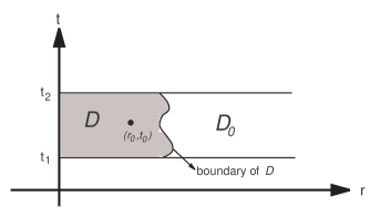
Figure 1: The considered domain with boundary, $\partial D$, which separates the interior domain $D$ and the vacuum domain $D_{0}$.

It is clear from the implicit definition of the boundary curve, $\partial D:\;\;r=B(t)$ that

$$M(B(t),t) \equiv m,$$

$$\dot{B}(t) = -\left[\frac{M_{,4}}{M_{,1}}\right]_{|\partial D}=\left[\frac{T^{1}_{\;4}}{T^{4}_{\;4}}\right]_{|\partial D}.$$ (12)

The spherical body collapses in case $M_{,4}(r,t)>0$ and expands in case $M_{,4}(r,t)<0$.

In case the measurable speed of the boundary is less than the speed of light, we must have:

$$e^{\alpha-\gamma}_{|\partial D}\left[\dot{B}(t)\right]^{2} < 1,$$

$$\left[e^{-\alpha}(M_{,1})^{2}-e^{-\gamma}(M_{,4})^{2}\right]_{|\partial D} > 0,$$ (13)

$$\left[\frac{T^{1}_{\;4}}{T^{4}_{\;4}}\right]^{2}_{|\partial D} < \left[1-\frac{2m}{B(t)}\right]^{2}\exp\left[h(t)+\chi(B(t),t)\right],$$

$$B(t) \neq 2m.$$

The interior domain $D$, the boundary $\partial D$ and the exterior (vacuum) domain $D_{0}$ are explained in the equations (6a),(6b) and (11) and in the figure 1. Following Synge, we shall now match continuously the interior metric to the exterior metric (transformable to the Schwarzschild chart). We must use the equations (10d), (10e) and (11) to arrive at:

$$g^{11}(r,t)=e^{-\alpha(r,t)}=\left\{\begin{array}[]{lll}1-\frac{2M(r,t)}{r}&\mbox{ for }&0<r<B(t),\;\;t_{1}<t<t_{2},\\ 1-\frac{2m}{B(t)}&\mbox{ for }&r=B(t),\;\;t_{1}<t<t_{2},\\ 1-\frac{2m}{r}&\mbox{ for }&B(t)<r<\infty,\;\;t_{1}<t<t_{2},\end{array}\right.$$ (14)

$$-g_{44}(r,t)=e^{\gamma(r,t)}=\left\{\begin{array}[]{lll}\left[1-\frac{2M(r,t)}{r}\right]\exp\left[h(t)+\chi(r,t)\right]&\mbox{ for }&0<r<B(t),\;\;t_{1}<t<t_{2},\\ \left[1-\frac{2m}{B(t)}\right]\exp\left[h(t)+\chi(B(t),t)\right]&\mbox{ for }&r=B(t),\;\;t_{1}<t<t_{2},\\ \left[1-\frac{2m}{r}\right]\exp\left[h(t)+\chi(B(t),t)\right]&\mbox{ for }&B(t)<r<\infty,\;\;t_{1}<t<t_{2}.\end{array}\right.$$ (15)

The exterior metric can be easily transformed to the Schwarzschild coordinates. We shall next investigate both Synge’s [1] and ISLD’s [3] junction conditions.

4 Junction conditions

4.1 Synge’s junction condition

Synge’s junction conditions read

$$T^{i}_{\;j}n_{i|\partial D} = 0,$$ (16)

$$n_{i}n^{i} = 1,$$

with $n^{i}$ a unit normal at the boundary. In the present case, with the help of (13) we can write for the relevant normal components:

$$n_{1}=\frac{M_{,1}}{\sqrt{e^{-\alpha}(M_{,1})^{2}-e^{-\gamma}(M_{,4})^{2}}}|_{\partial D},$$ (17)

$$n_{4}=\frac{M_{,4}}{\sqrt{e^{-\alpha}(M_{,1})^{2}-e^{-\gamma}(M_{,4})^{2}}}|_{\partial D}.$$

The equations (16) reduce to

$$\left[T^{1}_{\;1}M_{,1}+T^{4}_{\;1}M_{,4}\right]_{|\partial D} =0,$$ (18a)

$$\left[T^{1}_{\;4}M_{,1}+T^{4}_{\;4}M_{,4}\right]_{|\partial D} =0.$$ (18b)

By the equations (9b) and (9c), the junction condition (18b) is identically satisfied. Moreover, the other junction condition (18a) yields:

$$\left|\begin{array}[]{ll}T^{1}_{\;1}&T^{1}_{\;4}\\ T^{4}_{\;1}&T^{4}_{\;4}\end{array}\right|_{\partial D}=0$$

or,

$$\left[e^{\gamma-\alpha}T^{1}_{\;1}M_{,1}-T^{1}_{\;4}M_{,4}\right]_{|\partial D}=0.$$ (19)

There exist two possible cases here. In case the boundary is static, we must have from (12) and (19)

$$\dot{B}(t) \equiv 0,$$

$$T^{1}_{\;1}T^{4}_{\;4\,|\partial D} \equiv 0,$$ (20)

$$h(t) \mbox{is an arbitrary function}.$$ (21)

This case does not imply that the interior metric is necessarily static.

In case the boundary is non-static, we obtain from (9b), (9c), (12) and (19)

$$\dot{B}(t) \neq 0,$$

$$T^{1}_{\;1}T^{4}_{\;4|\partial D} < 0,$$

$$e^{h(t)} = \left[1-\frac{2m}{B(t)}\right]^{-2}\exp\left[-\chi(B(t),t)\right]\left[\dot{B}(t)\right]^{2}\left|\frac{T^{4}_{\;4}}{T^{1}_{\;1}}\right|_{\;|\partial D}>0.$$ (22)

Thus, the function $h(t)$, which originated as an arbitrary function of integration, can be utilized to satisfy the junction conditions.

4.2 Israel-Sen-Lanczos-Darmois junction condition

Next we consider the ISLD junction conditions. Namely, we consider the continuity of the second fundamental form at the junction. For this purpose, the three-dimensional metric for the hyper-surface corresponding to $\partial D\times S^{2}$ is obtained from (15) as

$$d\sigma^{2}:=ds^{2}_{|r=B(t)} = B^{2}(t)\left[d\theta^{2}+\sin^{2}\theta\,d\phi^{2}\right]$$ (23)

$$-\left\{\left[1-\frac{2m}{B(t)}\right]\exp\left[h(t)+\chi(B(t),t)\right]-\left[\dot{B}(t)\right]^{2}\right\}dt^{2}.$$

The extrinsic curvature components [11] calculated from the interior and exterior metrics are the following:

$$K_{\theta\theta}^{\pm} = \lim_{\delta\rightarrow 0_{+}}\left\{-\frac{re^{-\alpha}}{\sqrt{e^{-\alpha}-e^{-\gamma}\left[\dot{B}(t)\right]^{2}}}\right\}_{|r=B(t)\pm\delta},$$

$$K^{\pm}_{\phi\phi} = \sin^{2}\theta\,K^{\pm}_{\theta\theta},$$ (24)

$$2K^{\pm}_{tt} = \lim_{\delta\rightarrow 0_{+}}\left\{\frac{1}{\sqrt{e^{-\alpha}-e^{-\gamma}\left[\dot{B}(t)\right]^{2}}}\left[2\ddot{B}(t)+e^{\gamma-\alpha}\gamma_{,1}+\dot{B}(t)\left(2\alpha-\gamma\right)_{,4}\right.\right.$$

$$\left.\left.+\left[\dot{B}(t)\right]^{2}\left(\alpha-2\gamma\right)_{,1}-\left[\dot{B}(t)\right]^{3}e^{\alpha-\gamma}\alpha_{,4}\right]\right\}_{|r=B(t)\pm\delta}.$$

It is clear from (14), (15) and (23) that

$$K^{-}_{\theta\theta}-K^{+}_{\theta\theta} \equiv 0,$$ (25)

$$K^{-}_{\phi\phi}-K^{+}_{\phi\phi} \equiv 0.$$ (26)

To show the continuity of $K_{tt}$ across $\partial D$, we consider the function

$$2L^{\pm}:=\lim_{\delta\rightarrow 0_{+}}\left\{e^{\gamma-\alpha}\gamma_{,1}+\dot{B}(t)(2\alpha-\gamma)_{,4}+\left[\dot{B}(t)\right]^{2}(\alpha-2\gamma)_{,1}-\left[\dot{B}(t)\right]^{3}e^{\alpha-\gamma}\alpha_{,4}\right\}_{r=B(t)\pm\delta}.$$ (27)

The continuity of $L$ across $\partial D$ implies, from (15) and (4a - 4f), (after a long calculation) the following algebraic equation:

$$0 \equiv 2\kappa^{-1}\left[1-\frac{2m}{B(t)}\right]e^{h(t)+\chi(B(t),t)}\left[L^{-}-L^{+}\right]$$ (28)

$$= U(t)e^{2h(t)}+V(t)e^{h(t)}+W(t).$$

Here,

$$U(t) := B(t)\left[1-\frac{2m}{B(t)}\right]^{2}e^{2\chi(B(t),t)}T^{1}_{\;1|r=B(t)},$$

$$V(t) := -B(t)\dot{B}^{2}(t)\left\{e^{\chi(B(t),t)}\left(T^{1}_{\;1}-T^{4}_{\;4}\right)\right\}_{|r=B(t)},$$ (29)

$$W(t) := -B(t)\left[\dot{B}(t)\right]^{4}\left[1-\frac{2m}{B(t)}\right]^{-2}T^{4}_{\;4|r=B(t)}.$$

Analyzing the above quadratic (or possibly linear) equation for $e^{h(t)}$, we obtain the following solutions:

Case I: $$\;\;T^{1}_{\;1|\partial D}=\dot{B}(t)\,T^{4}_{\;4|\partial D}\equiv 0\;\mbox{ and }\;h(t)\;\mbox{ is arbitrary;}$$ (30a)

Case II: $$\;\;e^{h(t)}=\left[\dot{B}(t)\right]^{2}e^{-\chi(B(t),t)}\left[1-\frac{2m}{B(t)}\right]^{-2}\;\;\;\mbox{ for }\;\;\;\left\{\begin{array}[]{lll}i)\;T^{1}_{\;1|\partial D}\equiv 0,\;\;\dot{B}(t)T^{4}_{\;4|\partial D}\neq 0;\\ ii)\;\left(T^{1}_{\;1}-T^{4}_{\;4}\right)_{\partial D}=0;\\ iii)\;T^{1}_{\;1|\partial D}\neq 0,\;\;T^{4}_{\;4|\partial D}=0;\end{array}\right.$$ (30e)

Case III: $$\;\;T^{1}_{\;1|\partial D}>0,\;\;T^{4}_{\;4|\partial D}<0,\;\;\dot{B}(t)\neq 0,$$

$$\mbox{ and }\;\;e^{h(t)}=-\left[\dot{B}(t)\right]^{2}e^{-\chi(B(t),t)}\left[1-\frac{2m}{B(t)}\right]^{-2}\left|\frac{T^{4}_{\;4}}{T^{1}_{\;1}}\right|_{|\partial D}.$$ (30f)

It is clear that Synge’s conditions (21) and (22) satisfy the ISLD conditions (30a) and (30f). Case II represents a possible mathematical extension of the ISLD junction conditions to a non-time-like boundary.

5 Weak energy conditions

Next the weak energy conditions in spherical symmetry are studied. We consider an observer with an arbitrary boost which, to our knowledge, has not been calculated before.

In terms of the orthonormal components (denoted by indices in parentheses), the weak energy conditions [4] can be stated as

$$T_{(a)(b)}u^{(a)}u^{(b)}\geq 0$$ (31)

for every time-like vector $u^{(a)}$ satisfying

$$\left[u^{(1)}\right]^{2}+\left[u^{(2)}\right]^{2}+\left[u^{(3)}\right]^{2}-\left[u^{(4)}\right]^{2}=-1,$$ (32)

with $u^{(4)}>0$ as dictated by reasonable physics.

The general solution of the above non-linear algebraic equation (32) is given by:

$$u^{(1)} = \sinh\beta\cos\theta,\;u^{(2)}=\sinh\beta\sin\theta\cos\phi,\;u^{(3)}=\sinh\beta\sin\theta\sin\phi,\;u^{(4)}=\cosh\beta,$$

$$\beta \in \mathbb{R},\;\;\theta\in(0,\,\pi),\;\;\phi\in(-\pi,\,\pi).$$ (33)

For spherical symmetry, choosing the orthonormal basis of (3), the inequality (31) together with equations (33) yield:

$$\left[T_{(1)(1)}-T_{(2)(2)}\right]x^{2}y^{2}+T_{(2)(2)}x^{2}+2T_{(1)(4)}xy+T_{(4)(4)}\geq 0,$$ (34)

$$x:=\tanh\beta,\;\;y:=\cos\theta.$$

Analyzing the inequality (34) for all $(x,y)\in[-1,1]\times[-1,1]$, we conclude, after much calculation, that either

$$(i) \;\;T_{(1)(1)}\equiv T_{(2)(2)},\;T_{(1)(4)}\equiv 0,\;T_{(4)(4)}\geq 0,\;T_{(4)(4)}+T_{(1)(1)}\geq 0,$$ (35a)

or else

$$(ii) \;\;T_{(1)(1)}>T_{(2)(2)},\;\left(T_{(1)(4)}\right)^{2}\leq T_{(4)(4)}\left[T_{(1)(1)}-T_{(2)(2)}\right],$$

$$\;\left(T_{(1)(4)}\right)^{2}\leq\left[T_{(1)(1)}-T_{(2)(2)}\right]\left[T_{(4)(4)}+T_{(2)(2)}\right].$$ (35b)

We can solve the inequalities (35a) (35b) by utilizing slack functions:

$$T^{4}_{\;4}= T^{(4)}_{\;(4)}=-E^{2}(r,t),$$ (36a)

$$T^{2}_{\;2}= T^{(2)}_{\;(2)}=P^{2}(r,t)-\left[E(r,t)\sin Q(r,t)\right]^{2},$$ (36b)

$$T^{1}_{\;1}= T^{(1)}_{\;(1)}=P^{2}(r,t)-\left[E(r,t)\sin Q(r,t)\right]^{2}+H^{2}(r,t),$$ (36c)

$$e^{(\alpha-\gamma)/2}T^{1}_{\;4}= T_{(1)(4)}=-H(r,t)E(r,t)\cos Q(r,t)$$ (36d)

Here, the slack functions $E(r,t),\;P(r,t),\;Q(r,t),\;H(r,t)$ are of class $C^{1}$ but otherwise arbitrary.

6 Real eigenvalues of $\left[T^{i}_{\;j}\right]$ and anisotropic fluid models

First, we analyze and solve the problem of a spherically symmetric $T^{i}_{\;j}$ possessing real eigenvalues. Recall that the eigenvalue problem for $T^{i}_{\;j}$ is given by:

$$T^{i}_{\;j}\,E^{j}_{(a)}=\lambda_{(a)}E^{i}_{(a)}\;.$$ (37)

In the spherically symmetric case, $T^{1}_{\;2}=T^{1}_{\;3}=T^{2}_{\;4}=T^{3}_{\;4}\equiv 0,\;T^{2}_{\;2}\equiv T^{3}_{\;3}$. Therefore, the eigenvalues of $T^{i}_{\;j}$ are given by:

$$\lambda_{(2)} \equiv \lambda_{(3)}=T^{2}_{\;2},$$ (38)

$$2\lambda_{(1)} = T^{1}_{\;1}+T^{4}_{\;4}+\sqrt{\Delta},$$

$$2\lambda_{(4)} = T^{1}_{\;1}+T^{4}_{\;4}-\sqrt{\Delta},$$

$$\Delta: = \left(T^{1}_{\;1}-T^{4}_{\;4}\right)^{2}-e^{\alpha-\gamma}\left(T^{1}_{\;4}\right)^{2}.$$

It is clear that $\Delta<0$ will imply complex eigenvalues. We restrict ourselves in this section to the case where the stress-energy tensor possesses real eigenvalues ($\Delta\geq 0$).

In a static model, $T^{1}_{\;4}\equiv 0$ and $\Delta\geq 0$ is automatically valid. In case of the weak energy conditions in (35a), (35b) and the corresponding solutions in (36a - 36d),

$$\Delta=P^{4}+2P^{2}\left(H^{2}+E^{2}\cos^{2}Q\right)+(H-E^{2}\cos^{2}Q)^{2}\geq 0,$$ (39)

and thus real eigenvalues are guaranteed. (However, $\Delta\geq 0$ may not imply the weak energy conditions.)

Assuming the existence of real eigenvalues, the corresponding natural orthonormal eigenvectors are furnished by:

$$E^{i}_{(2)} = r^{-1}\delta^{i}_{(2)},E^{i}_{(3)}=(r\sin\theta)^{-1}\delta^{i}_{(3)},\;E^{1}_{(1)}=\frac{1}{2}\nu_{(1)}\left[T^{4}_{\;4}-T^{1}_{\;1}-\sqrt{\Delta}\right],$$

$$E^{2}_{(1)} = E^{3}_{(1)}\equiv 0,\;E^{4}_{(1)}=-\nu_{(1)}T^{4}_{\;1},E^{1}_{(4)}=-\nu_{(4)}T^{1}_{\;4},\;E^{2}_{(4)}=E^{3}_{(4)}\equiv 0,$$ (40)

$$E^{4}_{(4)} = \frac{1}{2}\nu_{(4)}\left(T^{1}_{\;1}-T^{4}_{\;4}+\sqrt{\Delta}\right),$$

$$\left[\nu_{(1)}\right]^{2} := \frac{2e^{-\alpha}}{\sqrt{\Delta}\left[T^{1}_{\;1}-T^{4}_{\;4}+\sqrt{\Delta}\right]},$$

$$\left[\nu_{(4)}\right]^{2} := \frac{2e^{-\gamma}}{\sqrt{\Delta}\left[T^{1}_{\;1}-T^{4}_{\;4}+\sqrt{\Delta}\right]}.$$

The decomposition of the spherically symmetric $T^{ij}$ in terms of the real eigenvalues and eigenvectors is accomplished by

$$T^{ij}=\left[\lambda_{(1)}-\lambda_{(2)}\right]E^{i}_{(1)}E^{j}_{(1)}+\lambda_{(2)}g^{ij}+\left[\lambda_{(2)}-\lambda_{(4)}\right]E^{i}_{(4)}E^{j}_{(4)}.$$ (41)

It is worth noting that the above algebraic structure of the stress-energy tensor is common to many different physical arenas. For example, the anisotropic fluid is specified by

$$p_{\shortparallel} := \lambda_{(1)},\;p_{\perp}:=\lambda_{(2)}\equiv\lambda_{(3)}=T^{2}_{\;2},\;\mu:=-\lambda_{(4)},$$

$$u^{i} := E^{i}_{(4)},\;s^{i}:=E^{i}_{(1)},$$

$$T^{ij} = \left(\mu+p_{\perp}\right)u^{i}u^{j}+p_{\perp}g^{ij}+\left(p_{\shortparallel}-p_{\perp}\right)s^{i}s^{j}.$$ (42)

The physical quantities are the energy density ($\mu$) the radial pressure ($p_{\shortparallel}$) and the angular or transverse pressures ($p_{\perp}$). Anisotropic fluid models have received much attention mainly in the arenas of stellar structure theory, black holes and cosmology [7], [12], [13], [14]. Note that the nomenclature “anisotropic fluid” is misleading. The stress-energy tensor in (42) actually represents a fluid which is not necessarily isotropic.

In case $\lambda_{(1)}\equiv\lambda_{(2)}\equiv\lambda_{(3)}$ (or $p_{\shortparallel}=p_{\perp}=:p$), the equation (42) yields the well known perfect fluid stress-energy tensor:

$$T^{ij}=\left(\mu+p\right)u^{i}u^{j}+pg^{ij}.$$ (43)

This equation implies, by equation (6d) and (38), the isotropy equation:

$$\sqrt{(T^{1}_{\;1}-T^{4}_{\;4})^{2}-e^{2\alpha-h-\chi}(T^{1}_{\;4})^{2}} = rT^{1}_{\;1,1}+\left[1-\frac{r}{2}\alpha_{,1}+\frac{\kappa r^{2}}{2}e^{\alpha}\left(T^{1}_{\;1}-T^{4}_{\;4}\right)\right]\left(T^{1}_{\;1}-T^{4}_{\;4}\right)$$ (44)

$$-e^{-(h+\chi)/2}\left[e^{2\alpha-(h+\chi)/2}T^{1}_{\;4}\right]_{,4}.$$

It is a formidable equation to solve in general (see [15] for detailed considerations of the static case.)

In case the spatial eigenvalues are identically zero, the stress-energy tensor in (42) reduces to that of an incoherent dust.

In case we identify $p=\lambda_{(2)}\equiv\lambda_{(3)},\;\mu=-\lambda_{(4)},\;\alpha:=\lambda_{(1)}-\lambda_{(2)}$, the stress-energy tensor is,

$$T^{ij}=(\mu+p)u^{i}u^{j}+pg^{ij}+\alpha s^{i}s^{j}.$$ (45)

The above $T^{ij}$ is due to a perfect fluid plus a tachyonic (space-like) dust. Such a stress-energy tensor has been considered in a cosmological model [13] where the dust contributes to the dark matter or dark energy component of the universe.

Now we are in a position to state and prove the main theorems of this section involving anisotropic fluids.

Theorem: 2.

Let the spherically symmetric interior equations (4a-4d) and the conservation equations (4e), (4f) hold in the coordinate convex domain $D$ defined by (5). Moreover, let the stress-energy tensor $T^{i}_{\;j}$ be that of an anisotropic fluid given by (42). Also, let the physical conditions $T^{4}_{\;4}\leq 0$ and $T^{1}_{\;1}-T^{4}_{\;4}\geq 0$ be satisfied in $D$. Then, the most general solutions of all the equations and inequalities are furnished by the following:

$$0<q_{1}<1 0<q_{2}<1,$$ , (46)

$$2M(r,t) := \kappa q_{1}\left\{F^{2}(q_{2}t)+\int_{0^{+}}^{r}E^{2}(x,q_{2}t)x^{2}\,dx\right\}>0,$$

$$e^{-\alpha(r,t)} = 1-\frac{2M(r,t)}{r},$$

$$e^{\gamma(r,t)} = e^{-\alpha(r,t)}\exp\left[h(t)+\chi(r,t)\right],$$

$$\chi(r,t) := \kappa q_{1}\int_{0^{+}}e^{\alpha(x,t)}\left[E^{2}(x,q_{2}t)\cos^{2}Q(x,q_{2}t)+P^{2}(x,q_{2}t)\right]x\,dx,$$

$$\Delta(r,t) = (q_{1})^{2}\left[E^{2}\cos^{2}Q+P^{2}\right]^{2}-\frac{4}{\kappa^{2}r^{4}}e^{\alpha-\gamma}\left(M_{,4}\right)^{2}\geq 0,$$

$$\frac{2}{q_{1}}\mu(r,t) = (q_{1})^{-1}\sqrt{\Delta}+E^{2}\left[1+\sin^{2}Q\right]-P^{2}\geq 0,$$

$$\frac{2}{q_{1}}p_{\shortparallel}(r,t) = (q_{1})^{-1}\sqrt{\Delta}-E^{2}\left[1+\sin^{2}Q\right]+P^{2}\geq 0,$$

$$\frac{p_{\perp}(r,t)}{q_{1}} = \frac{1}{2r}\left[r^{2}(P^{2}-E^{2}\sin^{2}Q)\right]_{,1}$$

$$+r\left\{\frac{1}{4}(E^{2}\cos^{2}Q+P^{2})\gamma_{,1}-(kq_{1})^{-1}e^{-(\alpha+\gamma)/2}\left[e^{(3\alpha-\gamma)/2}M_{,4}\right]_{,4}\right\}$$

$$u^{1} = -\frac{2\sqrt{2}}{\kappa e^{\gamma/2}r^{2}\Delta^{1/4}}\frac{M_{,4}}{\sqrt{q_{1}\left(E^{2}\cos^{2}Q+P^{2}\right)+\sqrt{\Delta}}},\;u^{2}=u^{3}\equiv 0,$$

$$u^{4} = \frac{1}{\sqrt{2}e^{\gamma/2}\Delta^{1/4}}\sqrt{q_{1}\left(E^{2}\cos^{2}Q+P^{2}\right)+\sqrt{\Delta}}>0,$$ (47)

$$s^{1} = \mp\frac{1}{\sqrt{2}e^{\alpha/2}\Delta^{1/4}}\sqrt{q_{1}\left(E^{2}\cos^{2}Q+P^{2}\right)+\sqrt{\Delta}},\;s^{2}=s^{3}\equiv 0,$$

$$s^{4} = \mp\frac{2\sqrt{2}e^{\alpha/2-\gamma}M_{,4}}{\kappa r^{2}\Delta^{1/4}\sqrt{q_{1}\left(E^{2}\cos^{2}Q+P^{2}\right)+\sqrt{\Delta}}}.$$

Here, the functions $F(q_{2}t),\;h(t),E(r,q_{2}t)$ (not identically zero) are of at least class $C^{3}$ in $D$. Aside from these restrictions, the functions are arbitrary.

For proof of the above theorem we used the equations (6a-6d), (10a - 10e), (36a-36d), (38), (40), (41) and (42). The two parameters in (46) may appear to be superfluous. However, note that in the limit $q_{1}\rightarrow 0_{+}$, the solutions in (46) yield the flat space metric. Moreover, for $0<q_{1}<1$ and and $\lim q_{2}\rightarrow 0_{+}$, the metric goes over to a static one. Furthermore, sufficiently small positive values of $q_{1}$ and $q_{2}$ facilitate satisfaction of the complicated inequalities $1-\frac{2M}{r}>0$ and $\Delta>0$.

We consider here a specific example of an exotic black hole. Consider the following:

$$F(q_{2}t) \equiv 0,\;E^{2}(r,q_{2}t):=\frac{jr^{j-3}}{(1-q_{2}t)^{j}},\;3\leq j.$$

$$2M(r,t) = \kappa q_{1}\left[\frac{r}{1-q_{2}t}\right]^{j},\;r=B(t):=\left(\frac{2m}{\kappa q_{1}}\right)^{1/j}\left(1-q_{2}t\right),$$

$$e^{-\alpha(r,t)} = \left[1-\frac{\kappa q_{1}r^{j-1}}{(1-q_{2}t)^{j}}\right],$$ (48)

$$T^{1}_{\;1}(r,q_{2}t) := k^{-2}q_{1}E^{2}(r,q_{2}t),\;\sqrt{3}\leq k,$$

$$\chi(r,q_{2}t) = -(1+k^{-2})\ln\left[1-\frac{\kappa q_{1}r^{j-1}}{(1-q_{2}t)^{j}}\right],$$

$$e^{\gamma(r,t)} = \left[1-\frac{\kappa q_{1}r^{j-1}}{(1-q_{2}t)^{j}}\right]^{-1/k^{2}}e^{h(t)}.$$

The above describes a mathematically rigorous collapse model for an anisotropic fluid black hole [7].

Now we shall consider the junction conditions for the solutions given in (48). We state and prove the following corollary to the preceding theorem.

Corollary:.

Let the conditions stated in the previous theorem be valid in $D$ with $E(r,q_{2}t)\neq 0$. Moreover, let both Synge’s junction conditions $T^{ij}M_{,j|\partial D}\equiv 0$ and the ISLD junctions conditions $\left[K_{ij}\right]_{\partial D}=0$ hold on $\partial D$. Then, either,

$$\sin^{2}Q(r,q_{2}t)\,E^{2}(r,q_{2}t)= P^{2}(r,q_{2}t)+\left[B(t)-r\right]^{\nu^{2}}N(r,q_{2}t)\geq 0,\nu^{2}\in\left\{1,2\right\}\cup[3,\infty)$$

and

$$F^{2}(q_{2}t)= (c_{0})^{2}+\int_{t}^{t_{2}}d\tau\left\{\int_{0_{+}}^{B(t)}x^{2}\frac{\partial}{\partial\tau}\left[E^{2}(x,q_{2}\tau)\right]\,dx\right\}\geq 0,$$ (49a)

or else

$$F^{2}(q_{2}t)= f^{2}(q_{2}t)+\int_{t}^{t_{2}}d\tau\left\{\int_{0_{+}}^{B(t)}x^{2}\frac{\partial}{\partial\tau}\left[E^{2}(x,q_{2}\tau)\right]\,dx\right\},$$ (49b)

$$E^{2}(r,q_{2}t)= \frac{P^{2}}{{\rm\mbox{{sech}}}^{2}\left[R(r,q_{2}t)\right]+\sin^{2}Q}>0,\;\dot{f}(q_{2}t)\neq 0,$$

and

$$e^{h(t)}= 4\left\{(1-\frac{2m}{r})^{-2}e^{-\chi(r,t)}\left[\frac{M_{,4}\cosh(R(r,q_{2}t))}{\kappa q_{1}r^{2}E^{2}(r,q_{2}t)}\right]^{2}\right\}_{|r=B(t)}>0.$$

Here, $N(r,q_{2}t),\;R(r,q_{2}t)$ and $f(q_{2}t)$ are functions of at least class $C^{3}$ in $D$ but otherwise arbitrary.

Proof: By the equations (36c) and (49a) it follows that

$$(q_{1})^{-1}T^{1}_{\;1}=-\left[B(t)-r\right]^{\nu^{2}}N(r,q_{2}t),\;T^{1}_{\;1|r=B(t)}\equiv 0.$$

Furthermore,

$$\left[\frac{2M_{,4}}{\kappa q_{1}}\right]_{|r=B(t)}=\frac{dF^{2}(q_{2}t)}{dt}+\int_{0^{+}}^{B(t)}x^{2}\frac{\partial}{\partial t}E^{2}(x,q_{2}t)\,dx\equiv 0.$$

Therefore, by (21) and (30a), both Synge’s condition and the ISLD conditions are satisfied.

In the second case, by the equations in (36c) and (49b) it is deduced that

$$\kappa^{-1}T^{1}_{\;1}(r,q_{2}t)=P^{2}-E^{2}(r,q_{2}t)\sin^{2}Q=E^{2}(r,q_{2}t)\mbox{sech}^{2}\left[R(r,q_{2}t)\right]>0.$$ (50)

Moreover, $M_{,4}\neq 0$ and

$$e^{h(t)}=\left(1-\frac{2m}{r}\right)^{-2}e^{-\chi(r,t)}\left[\frac{(T^{1}_{\;4})^{2}}{-T^{4}_{\;4}T^{1}_{\;1}}\right]_{|r=B(t)}.$$

Thus, both equations (22) and (30f) are satisfied. $\blacksquare$

We have previously proved [8] that under the two conditions $T^{1}_{\;4}\equiv 0$ and $T^{1}_{\;1,4}\equiv 0$, the solutions of the equations (4a-4f) can be transformed into a static solution. This is the interior version Birkhoff’s theorem. We can investigate directly the static limit of equations (4a-4f). Under suitable assumptions, including $\frac{dM(r)}{dr}>0$, the boundary, $\partial D$, of the spherical body is given by $r=b$, a positive constant. Now, the general solution will be furnished in the following statement:

Theorem: 3.

Let the static version of the spherically symmetric field equations and one conservation law (4a-4f) hold in the domain $D:=\left\{(r,t):0<r<b,\;t_{1}<t<t_{2}\right\}$. Moreover, let the stress-energy tensor be given by (42), satisfying $\mu(r)>0,\;\mu(r)+p_{\shortparallel}>0$. If, in addition, both Synge’s and the ISLD junction conditions hold at $r=b$, then the general solutions of the static equations are furnished by:

$$0<q_{1}<1 b>0,\;c_{0}\in\mathbb{R},\;\nu^{2}\in\left\{1,2\right\}\cup[3,\infty),$$ ,

$$2M(r) = \kappa\left[(c_{0})^{2}+\int_{0}^{r}x^{2}\mu(x)\,dx\right]>0,$$

$$e^{-\alpha(r)} = 1-\frac{2M(r)}{r},$$

$$\chi(r) := \kappa\int_{0^{+}}^{r}e^{\alpha(x)}\left[\mu(x)+p_{\shortparallel}(x)\right]x\,dx,$$

$$e^{\gamma(r)} = e^{\chi(r)-\alpha(r)},$$ (51)

$$\Delta(r) = \left[\mu(r)+p_{\shortparallel}(r)\right]^{2}>0,$$

$$\mu(r) = q_{1}E^{2}(r)>0,\;p_{\shortparallel}=q_{1}\left[P^{2}(r)-\left(\sin^{2}Q(r)\right)E^{2}(r)\right],$$

$$p_{\perp} = \frac{1}{2r}\left\{r^{2}p_{\shortparallel\,,1}+\frac{r}{4}p_{\shortparallel}\gamma_{,1}\right\},$$

$$u^{i} = e^{-\gamma(r)/2}\,\delta^{i}_{(4)},\;s^{i}=\pm e^{\alpha(r)/2}\delta^{i}_{(1)},$$

$$(\sin^{2}Q(r))E^{2}(r) := P^{2}(r)+(b-r)^{\nu^{2}}N(r)>0.$$

Here, $E(r)$, $P(r)$, $Q(r)$ and $N(r)$ are functions of at least class $C^{3}$. Moreover, these functions and the parameters $c_{0}$ and $\nu$ are arbitrary save for the restrictions imposed above.

Proof follows from (46) and (49a). Note that to avoid a singularity at $r=0$ (if this is included in the domain), the constant $c_{0}$ should be set equal to zero so that $\lim_{r\rightarrow 0}M(r)=0$.

An illustrative example will be provided in the following:

$$0<q_{1}<1, b>0,\;c_{0}=0,$$

$$E^{2}(r):=3, 2M(r)=\kappa q_{1}r^{3},$$

$$3\sin^{2}Q(r) := P^{2}(r)-3\kappa q_{1}(b-r)\times$$

$$\times\left\{\frac{b+r}{\left[3\sqrt{1-\kappa q_{1}b^{2}}-\sqrt{1-\kappa q_{1}r^{2}}\right]\left[\sqrt{1-\kappa q_{1}r^{2}}+\sqrt{1-\kappa q_{1}b^{2}}\right]}\right\}>0,$$

$$e^{\alpha(r)} = 1-\kappa q_{1}r^{2},$$

$$e^{\gamma(r)} = \left[\frac{3\sqrt{1-\kappa q_{1}b^{2}}-\sqrt{1-\kappa q_{1}r^{2}}}{3\sqrt{1-\kappa q_{1}b^{2}}-1}\right]^{2},$$

$$\mu(r) = 3q_{1},\;p_{\shortparallel}\equiv p_{\perp}=:p(r)=3q_{1}\left[\frac{\sqrt{1-\kappa q_{1}r^{2}}-\sqrt{1-\kappa q_{1}b^{2}}}{3\sqrt{1-\kappa q_{1}b^{2}}-\sqrt{1-\kappa q_{1}r^{2}}}\right],$$

$$p(b) = 0.$$ (52)

The above obviously yields the well known interior Schwarzschild constant density solution.

One final example which illustrates the use of this scheme is that of the inner layers of a static neutron star [16]. In this case, the energy density, $\mu=T_{(4)(4)}=-T^{4}_{\;4}$ is known from the quantum mechanics of degenerate Fermions. As well, there is the ultra-relativistic fluid equation of state, which should be valid in the inner layers of the star. We summarize as follows:

$$\mu(k_{F})=\frac{8\pi^{2}}{h^{3}}\int_{0}^{k_{F}}k^{2}(k^{2}+m_{n}^{2})^{1/2}\,dk$$

Here $h$ is Planck’s constant, $k_{F}$ is the Fermi-momentum and $m_{n}$ is the neutron mass. Since the extreme relativistic limit is employed, the mass terms may be neglected compared to the Fermi momentum so that a pressure calculation gives:

$$p_{\shortparallel}\equiv p_{\perp}=\frac{1}{3}\mu.$$ (53)

Also, $\mu(r)$ is obtained by utilizing (53) along with the linear combination $G^{1}_{\;1}-G^{4}_{\;4}=\frac{2}{3}\kappa\mu(r)$. Now the isotropy equation (44) of the general solution reads, in terms of $\mu(r)$,

$$\mu(r)_{,r}=-\frac{4}{r^{2}}\mu(r)\left[1-\frac{2M(r)}{r}\right]^{-1}\left[\frac{\kappa\mu(r)r^{3}}{6}+M(r)\right],$$ (54)

Noting relation (9b) and assuming a series solution in $r$ we arrive at the following:

$$M(r)=\frac{3}{14}r,\;\mu(r)=\frac{3}{7\kappa r^{2}},$$

which, from (6a) and (6b) yields:

$$e^{\gamma}=\frac{4}{7}\frac{r}{r_{0}},\;e^{\alpha}=\frac{7}{4}$$ (55)

with $r_{0}$ a constant. The neighborhood about $r=0$ is excised as the singularity at this point is due to the ultra-relativistic approximation. Also, this solution is not valid for outer layers of the star where deviations from the ultra-relativistic case are significant.

7 Exotic spherically symmetric solutions

The exact solutions in (10a - 10e) can be generalized by abandoning the weak energy conditions to express:

$$2\kappa^{-1}M(r,t)= f^{2}(t)-\int_{0^{+}}^{r}T^{4}_{\;4}(x,t)x^{2}\,dx,$$ (56a)

$$e^{-\alpha(r,t)}= 1-\frac{2M(r,t)}{r}>0,$$ (56b)

$$e^{\gamma(r,t)}= \left[1-\frac{2M(r,t)}{r}\right]e^{\chi(r,t)}H(t),$$ (56c)

$$\chi(r,t):= \kappa\int_{0^{+}}^{r}e^{\alpha(x,t)}\left[T^{1}_{\;1}(x,t)-T^{4}_{\;4}(x,t)\right]x\,dx,$$ (56d)

$$H(t)\neq 0.$$ (56e)

There are many situations when the solutions to these equations may prove to be “exotic” in some sense. For example, the equations (56b-56e) reveal that the condition signature$[g_{ij}]=+2$ may not be preserved everywhere. A simple example may be considered in the exact vacuum metric given by:

$$ds^{2}=\left(1-\frac{2m}{r}\right)^{-1}\,dr^{2}+r^{2}\left(d\theta^{2}+\sin^{2}\theta\,d\phi^{2}\right)+\left(1-\frac{2m}{r}\right)t^{3}\,dt^{2}.$$ (57)

In case $t<0$, the metric is obviously transformable to the Schwarzschild solution. However, for $t>0$ the line element (57) yields the spherically symmetric vacuum gravitational instanton solution. In (57), $\lim_{t\rightarrow 0}g_{44}(r,t)=0$, indicating the existence of a horizon. All the null rays from the Schwarzschild universe suddenly halt on such a horizon. It may be called the instanton horizon. Signature changing metrics in general relativity have been studied in [7], [17]. The most general spherically symmetric instanton solution in curvature coordinates is furnished by the equations (56a - 56e)with the choice $H(t)=-e^{h(t)}<0$.

Next, consider spherically symmetric $T$-domain solutions ([6] and references therein). The metric is locally expressible as:

$$ds^{2}= e^{\lambda(T,R)}\,dR^{2}+T^{2}\left(d\theta^{2}+\sin^{2}\theta\,d\phi^{2}\right)-e^{\nu(T,R)}\,dT^{2};$$ (58)

$$D_{T}:= \left\{(T,R):\;T_{1}<T<T_{2},\;R_{1}<R<R_{2}\right\}.$$

Einstein’s field equations $G^{i}_{\;j}+\kappa\Theta^{i}_{\;j}=0$ can be solved with the metric (58). The general solution (“dual” to the solutions in (6a - 6d)), is furnished by:

$$e^{-\nu(T,R)}= \frac{1}{T}\left[\sigma(R)-\kappa\int_{T_{0}}^{T}(T^{\prime})^{2}\Theta^{1}_{\;1}(T^{\prime},R)\;dT^{\prime}\right]-1=:\frac{2\Xi(T,R)}{T}-1>0\,,$$ (59a)

$$e^{\lambda(T,R)}= \left[\frac{2\Xi(T,R)}{T}-1\right]\exp\left\{\beta(R)+\kappa\int_{T_{0}}^{T}e^{\nu(T^{\prime},R)}\left[\Theta^{4}_{\;4}(T^{\prime},R)-\Theta^{1}_{\;1}(T^{\prime},R)\right]T^{\prime}\,dT^{\prime}\right\},$$ (59b)

$$\Theta^{4}_{\;1}(T,R):= \frac{2}{\kappa T^{2}}\left[\Xi(T,R)\right]_{,1},$$ (59c)

$$\Theta^{2}_{\;2}\equiv\Theta^{3}_{\;3}= \frac{T}{2}\left[\Theta^{4}_{\;4,4}+\Theta^{1}_{\;4,1}\right]+\left[1+\frac{T}{4}\lambda_{,4}\right]\Theta^{4}_{\;4}+\frac{T}{4}\left(\lambda+\nu\right)_{,1}\Theta^{4}_{\;1}-\frac{T}{2}\alpha_{,4}\Theta^{1}_{\;1},$$ (59d)

all other $$\Theta^{i}_{\;j}\mbox{'s}\equiv 0.$$

Here, the functions $\sigma(R)$ and $\beta(R)$ are of class $C^{3}$ but otherwise arbitrary. The “total tension” function, $\Xi(T,R)$ is generated by the tension density since, in the $T$-domain, it is $\Theta^{1}_{\;1}$ which appears in (59a). This class of solutions includes eternal black hole solutions.

Another special case of $T$-domain solutions occurs whenever the stress-energy tensor matrix $\left[\Theta^{i}_{\;j}\right]$ admits complex eigenvalues. The algebraic criterion of such occurrence is provided by the strict inequality:

$$\Delta^{\sharp}:=\left(\Theta^{4}_{\;4}-\Theta^{1}_{\;1}\right)^{2}+4\Theta^{1}_{\;4}\Theta^{4}_{\;1}<0.$$ (60)

As an example, the following $\Theta^{i}_{\;j}$ has appeared in the late stages of gravitational collapse studies [7]:

$$0<q_{1}<1,\; \;0<q_{2}<1,\;3\leq j,\;\sqrt{3}\leq k,$$

$$\Theta^{1}_{\;1}(T,R)= -\frac{jq_{1}T^{j-3}}{\left(1-q_{2}R\right)^{j}}<0,$$

$$\Theta^{4}_{\;4}(T,R)= k^{-2}jq_{1}\frac{T^{j-3}}{(1-q_{2}R)^{j}}>0,$$ (61)

$$\Theta^{4}_{\;1}(T,R)= \frac{jq_{1}q_{2}T^{j-2}}{\left(1-q_{2}R\right)^{j}}>0.$$

Finally, we shall consider the spherically symmetric field equations in an arbitrary $D$-dimensional manifold (with $D\geq 3$) [8]. There has been much study on the possibility of extra dimensions in light of superstring theories. In the low energy sector, many of these theories reproduce a higher dimensional general relativity in which, above some energy scale, all dimensions may be considered non-compact. These higher dimensional field equations may therefore have relevance in these theories.

The metric in curvature coordinates is provided by:

$$ds^{2}=e^{\alpha(r,t)}\,dr^{2}+r^{2}\,d\Omega^{2}_{(D-2)}-e^{\gamma(r,t)}\,dt^{2}\;,$$ (62)

with

$$d\Omega^{2}_{(D-2)}= \left[d\theta_{(0)}^{2}+\sum_{n=1}^{D-3}d\theta_{(n)}^{2}\left(\prod_{m=1}^{n}\sin^{2}\theta_{(m-1)}\right)\right].$$

$$\tilde{D}:= \left\{(r,\;\theta_{(0)},\ldots,\theta_{(D-3)},\;t)\in\mathbb{R}^{D}:\;\;t_{1}<t<t_{2},\;0<r_{1}<r<r_{2},\right.$$

$$\left.\;0<\theta_{(0)},\ldots,\theta_{(D-4)}<\pi,\;0\leq\theta_{(D-3)}<2\pi\right\}.$$ (63)

The $D$-dimensional field equations and conservation laws read:

$$\mathcal{E}^{1}_{\;1}= \frac{D-2}{2r^{2}}\left[(D-3)\left(1-e^{-\alpha}\right)-re^{-\alpha}\gamma_{,1}\right]+\kappa T^{1}_{\;1}=0\;,$$ (64a)

$$\mathcal{E}^{2}_{\;2}= -\frac{e^{-\gamma}}{4}\left[\gamma_{,4}\alpha_{,4}-\left(\alpha_{,4}\right)^{2}-2\alpha_{,44}\right]\left.-\frac{e^{-\alpha}}{4}\left[2\gamma_{,11}+\left(\gamma_{,1}\right)^{2}+\frac{2(D-3)}{r}\left(\gamma-\alpha\right)_{,1}\right.\right.$$

$$\left.-\gamma_{,1}\alpha_{,1}+\frac{2}{r^{2}}(D-3)(D-4)\right]+\frac{2(D-3)(D-4)}{r^{2}}+\kappa T^{2}_{\;2}=0.$$ (64b)

$$\mathcal{E}^{4}_{\;1}= \frac{D-2}{2r}e^{-\gamma}\alpha_{,4}+\kappa T^{4}_{\;1}=0\;,\;\;\mathcal{E}^{\theta_{n}}_{\;\theta_{n}}\equiv\mathcal{E}^{2}_{\;2},$$ (64c)

$$\mathcal{E}^{4}_{\;4}= \frac{D-2}{2r^{2}}\left[(D-3)\left(1-e^{-\alpha}\right)+re^{-\alpha}\alpha_{,1}\right]+\kappa T^{4}_{\;4}=0\;,$$ (64d)

$$\mathcal{T}^{1}= T^{1}_{\;1,1}+T^{4}_{\;1,4}+\left[\frac{1}{2}\gamma_{,1}+\frac{D-2}{r}\right]T^{1}_{\;1}+\frac{1}{2}\left(\gamma+\alpha\right)_{,4}T^{4}_{\;1}-\left[\frac{1}{2}\gamma_{,1}T^{4}_{\;4}+\frac{D-2}{r}T^{2}_{\;2}\right]=0,$$ (64e)

$$\mathcal{T}^{4}= T^{4}_{\;4,4}+T^{1}_{\;4,1}+\frac{1}{2}\alpha_{,4}\left(T^{4}_{\;4}-T^{1}_{\;1}\right)+\frac{1}{2}T^{1}_{\;4}\left[\left(\alpha+\gamma\right)_{,1}+\frac{2(D-2)}{r}\right]=0,$$ (64f)

The general solution of the Einstein field equations and conservation equations furnished utilizing the scheme in this paper is:

$$e^{-\alpha(r,t)}= 1+\frac{2\kappa}{(D-2)r^{D-3}}\int_{r_{1}}^{r}T^{4}_{\;4}(x,t)x^{D-2}\,dx-\frac{\kappa f^{2}(t)}{r^{D-3}}=:1-\frac{2M(r,t)}{r^{D-3}},$$ (65a)

$$e^{\gamma(r,t)}= e^{-\alpha(r,t)}\exp\left\{h(t)+\frac{2\kappa}{D-2}\int_{r_{1}}^{r}\left[\frac{T^{1}_{\;1}(x,t)-T^{4}_{\;4}(x,t)}{x^{D-3}-2M(x,t)}\right]x^{D-2}\,dx\right\}.$$ (65b)

Again, the functions $f(t)$ and $h(t)$ are of class $C^{3}$ but otherwise arbitrary.

8 Concluding remarks

In summary, the general solution to the spherically symmetric Einstein field equations was provided in the case when the energy density and parallel pressure are known. Both Synge’s junction conditions and the Israel-Sen-Lancsoz-Darmois junction conditions have been studied and solved in general. The junction or boundary is defined by the existence of a total interior mass which has been rigorously proved in section 3. The weak energy conditions in spherical symmetry for arbitrary boost were presented and solved utilizing slack function methods. Specific matter models have also been considered including the anisotropic fluid satisfying both junction conditions, which includes the perfect fluid as a special case. Finally, exotic extensions were considered.

References

• [1] J. L. Synge, Relativity: The General Theory (North-Holland, Amsterdam, 1964);
Relativity, Groups and Topology (Les Houches 1963) (Gordon and Breach Science Publishers, New York, 1964).
• [2] R. C. Buck, Advanced Calculus (McGraw-Hill Book Co., New York, 1956).
• [3] W. Israel, Nuovo Cimento B44, 1 (1966);
N. Sen,
Ann. Phys. 73, 365 (1924);
K. Lanczos,
ibid. 74, 518 (1924);
G. Darmois,
Memorial des Sciences Mathematics XXV (Gauthier-Villars, Paris, 1927).
• [4] S. W. Hawking and G. F. R. Ellis, The Large Scale Structure of Space-Time (Cambridge University Press, Cambridge, 1973).
• [5] S. Kloster, M. M. Som and A. Das, J. Math. Phys. 15, 1096 (1974);
S. W. Hawking,
Phys. Lett. A 60, 81 (1977).
• [6] I. D. Novikov, Commun. Shternberg State Astron. Inst. 132, 3 (1964);
V. A. Ruban,
J.E.T.P. 29, 1027 (1969);
ibid. 58, 463 (1983);
E. Poisson and W. Israel,
Class. Quant. Grav. 5, L201 (1998);
A. DeBenedictis, D. Aruliah and A. Das,
Gen. Rel. Grav. 34, 365 (2002);
A. Burinskii, E. Elizalde, S. R. Hildebrandt and G. Magli,
Phys. Rev. D65, 064039 (2002);
E. Elizalde and S. R.Hildebrandt,
Phys. Rev. D65, 124024 (2002).
• [7] A. Das, N. Tariq and T. Biech, J. Math. Phys. 36, 340 (1995);
A. Das, N. Tariq and D. Aruliah,
J. Math. Phys. 38, 4202 (1997).
• [8] A. Das and A. DeBenedictis, Prog. Theor. Phys. 108, 119 (2002).
• [9] P. G. Bergmann, M. Cahen and A. B. Komar, J. Math. Phys. 6, 1 (1965);
H. J. Schmidt,
Grav. Cos. 3, 185 (1997);
K. A. Bronnikov and V. N. Melnikov,
Gen. Rel. Grav. 27, 465 (1995).
• [10] M. Spivak, Calculus on Manifolds (The Benjamin/Cummings Publishing Co., Menlo Park, 1965).
• [11] L. P. Eisenhart, Riemannian Geometry (Princeton University Press, Princeton, 1966).
• [12] A. Lichernowicz, Relativistic Hydrodynamics and Magnetohydrodynamics (Benjamin, New York, 1967);
L. Herrera and J. Ponce de Léon,
J. Math. Phys. 26, 2018, 2847 (1985).
• [13] A. Das and A. DeBenedictis, gr-qc/0304017. In press.
• [14] D. J. McManus and A. A. Coley, Class. Quant. Grav. 11, 2045 (1994);
H. Hernandez and L. A. Núñez,
Proceedings of the 9th Marcel Grossman Meeting and gr-qc/0012019 (2000);
L. Herrera, A. DiPrisco, J. Ospino and E. Fuenmayor
J. Math. Phys. 42, 2129 (2001);
T. Papakostas,
Int. J. Mod. Phys. D10, 869 (2001);
B. V. Ivanov,
Phys. Rev. D65, 104011 (2002);
L. Herrera, J. Martin and J. Ospino,
J. Math. Phys. 43, 4889 (2002);
H. Dehnen, V. D. Ivashuk and V. N. Melnikov,
gr-qc/0211049 (2002)
K. Dev and M. Gleiser,
Gen. Rel. Grav. 34, 1793 (2002);
M. K. Mak and T. Harko,
Proc. Roy. Soc. Lond. A459, 393 (2003);
K. A. Bronnikov, A. Dobsz and I. G. Dymnikov,
gr-qc/0302029 (2003);
L. P. Chimento,
gr-qc/0304033 To appear in Phys. Rev. D (2003).
• [15] D. Martin and M. Visser, gr-qc/0306109 (2003).
• [16] S. Weinberg, Gravitation and Cosmology: Principles and Applications of the General Theory of Relativity (Wiley, New York, 1972).
• [17] T. Dray, C. A. Manogue and R. W. Tucker, Phys. Rev. D48, 2587 (1993);
J. Martin,
Phys. Rev. D49, 5086 (1994);
C. Hellaby and T. Dray,
Phys. Rev. D49, 5096 (1994);
M. Carfora and G. F. R. Ellis,
Int. J. Mod. Phys. D4, 175 (1995);
S. A. Hayward,
gr-qc/9509052 (1995);
M. Kriele and J. Martin,
Class. Quant. Grav. 12, 503 (1995);
L. J. Alty, C. J. Fewster,
Class. Quant. Grav. 13, 1129 (1996);
F. Embacher,
Class. Quant. Grav. 13, 921 (1996);
T. Dray,
J. Math. Phys. 37, 5627 (1996);
T. Dray, G. Ellis, C. Hellaby, C. Manogue,
Gen. Rel. Grav. 29, 591 (1997);
R. Mansouri, K. Nozari,
gr-qc/9806109 (1998);
M. Mars, J. M. M. Senovilla, R. Vera,
Phys. Rev. Lett. 86, 4219 (2001);
A. K. Guts and M. S. Shapovalova,
Grav. Cos. 7, 193 (2001);
B. Z. Iliev,
Physica Scripta 66, 401 (2002);
T. Hirayama and B. Holdom,
hep-th/0303174 (2003).
• [18]