A gravitational memory effect in “boosted” black hole perturbation theory.

Abstract

Black hole perturbation theory, or more generally, perturbation theory on a Schwarzschild bockground, has been applied in several contexts, but usually under the simplifying assumption that the ADM momentum vanishes, namely, that the evolution is carried out and observed in the “center of momentum frame”. In this paper we consider some consequences of the inclusion of a non vanishing ADM momentum in the initial data. We first provide a justification for the validity of the transformation of the initial data to the “center of momentum frame”, and then analyze the effect of this transformation on the gravitational wave amplitude. The most significant result is the possibility of a type of gravitational memory effect that appears to have no simple relation with the well known Christodoulou effect.

I Introduction

Following its successful application to the close limit of head on collisions, by Price and Pullin PrPu , black hole perturbation theory has become an important tool in the analysis of the final stages of the coalescence of two black holes, after their collision or final plunge from their innermost stable orbit PuKy . In this context, the theory, originally formulated in the Fourier transformed frequency domain by Regge and Wheeler ReWhe and Zerilli Zerilli , is considered in the time domain as a manner of (perturbatively) solving an initial value problem. Namely, one is given initial data (a solution of the constraint equations of General Relativity) in the form of the 3-metric and extrinsic curvature on (some region of) a three dimensional spacelike hypersurface $\Sigma$ and the problem is to find the full metric in the domain of dependence of the initial data. The type of data considered here depends in general on one or more perturbation parameters $\epsilon_{i}$, in such a way that one recovers that for a Schwarzschild black hole when the $\epsilon_{i}$ vanish. The possibility of a perturbative analysis of the evolution is based on the expansion of the data in an appropriately chosen angular basis (tensor spherical harmonics), and the assumption that the angular component coefficient functions can be further expanded in powers of the $\epsilon_{i}$. The non trivial part of the Einstein equations can then be cast in the form of an infinite set of coupled partial differential equations for functions of two variables (conventionally, the Schwarzschild coordinates $t$ and $r$), that can, in principle, be integrated order by order in the perturbation parameters physrep . This, however, does not take into account the invariance of the geometry under coordinate changes. In fact, when this invariance is fully accounted for, the relevant physical information ends up being encoded in two sets of functions, where each element corresponds to an angular mode, introduced respectively by Regge and Wheeler ReWhe , and by Zerilli Zerilli , that satisfy wavelike equations in $t,r$.

While the above analysis, leading to the emergence of the Regge - Wheeler and the Zerilli functions is based on the general invariance of the theory under coordinate transformations, in recent applications to the black hole binary problem one is interested in the evolution of a given initial data, posed on a given hypersurface $\Sigma$. In perturbation theory, a particular choice is made of the zeroth order (in the $\epsilon_{i}$) coordinates. This still leaves the freedom of choice of coordinates within $\Sigma$, which can be redefined, provided this introduces changes of the same order as the perturbations moncrief . This gauge freedom on $\Sigma$ is very important because it allows to cast the evolution problem (and corresponding initial data) in different physically equivalent forms, that simplify either the mathematical treatment or the physical interpretation physrep .

However, in considering more general coordinate transformations one is faced with the following problem. Suppose that for certain choice of coordinates $x^{\mu}=(t,r,\theta,\phi)$, $\Sigma$ is the hypersurface $t=0$, and that the hypersurfaces $\Sigma_{t}$, corresponding to constant values of $t$ define a foliation of the space time manifold $\cal{M}$, as would be appropriate for the evolution of initial data on $\Sigma$, using $t$ as the “time” parameter. We may introduce now a different coordinate system, say $\tilde{x}^{\mu}=(\tilde{t},\tilde{r},\tilde{\theta},\tilde{\phi})$, such that the constant $(\tilde{t}$ hypersurfaces provide a different foliation of $\cal{M}$, but where the transformation between $\tilde{x}^{\mu}$ and $x^{\mu}$ depends on the $\epsilon_{i}$ in such a way that we get $\tilde{x}^{\mu}={x}^{\mu}$ for $\epsilon_{i}=0$. It is not immediate that this more general case can be treated as that where we consider coordinate changes only within $\Sigma$. This is because, by definition, the initial value problem, and corresponding initial data, for the coordinates $\tilde{x}^{\mu}$ correspond now to constant $\tilde{t}$, but the restrictions on the limits of the $\epsilon_{i}=0$, do not necessarily imply that, for finite $\epsilon_{i}$, even if the hypersurfaces $\Sigma$ and $\tilde{\Sigma}$, corresponding respectively to $t=0$ and $\tilde{t}=0$ intersect at some points, they cannot become widely separated in time as we move away from these points. (See below for more details). But this would imply, in principle, that in this case the only way we can implement the coordinate transformation is if we have already solved the evolution equations, since a finite amount of time is required to move in general from a point in $\Sigma$ to a point in $\tilde{\Sigma}$.

The previous discussion is relevant to the following problem. Suppose we are given a family of initial data for the Einstein equations, (3-metrics $g_{ij}$, extrinsic curvatures $K_{ij}$), depending smoothly on a parameter $P$, such that for $P=0$ we recover Schwarzschild’s space time, and for $P\neq 0$ the initial data is asymptotically flat, with ADM momentum $P$. Quite generally, for small $P$, we expect this data to evolve into a “boosted” Schwarzschild black hole, possibly accompanied with the emission of a certain amount of gravitational radiation. However, if we consider applying the Regge-Wheeler-Zerilli perturbation theory to analyze this evolution, we are faced with the problem that this theory is based on the assumption that the evolution leads to a stationary black hole, essentially centered at the origin of spatial coordinates, while the “natural” evolution of the given initial data leads to a non stationary final state of the black hole. Clearly, this problem could be solved by choosing a new foliation, where the final state of the black hole is stationary, but such transformation, for any $P\neq 0$ involves a “Lorentz boost”, with arbitrarily large separations of the hypersurfaces $\Sigma$ and $\tilde{\Sigma}$, as can be seen by considering the simpler similar case in Minkowski spacetime.

The evolution of conformally flat “boosted” single black hole initial data in black hole perturbation theory, was analyzed in a recent paper by Khanna, Gleiser and Pullin KhGlPu , (referred as I in what follows), but there the previous problem was given only a heuristic treatment. In more detail, the analysis performed in I makes use of second order perturbation theory, not as regards evolution, but rather to carry out a second order gauge transformation that eliminates the first order terms, leaving only the second order contributions, which then satisfy linearized Einstein equations. Although the results obtained regarding radiate wave forms are qualitatively in agreement with other results obtained in perturbation theory, i.e., they show, for instance, the expected “quasi-normal ringing”, an intriguing feature that distinguishes this case is that the Zerilli function $\psi$ does not vanish for large radial distance, approaching instead a constant non vanishing value. Since the radiated energy depends on the time derivative of $\psi$, the presence of this constant does not in itself mean that there is a divergence, but this behavior is in clear contrast with that previously observed in other applications of perturbation theory, and, therefore, it justifies a more detailed analysis and interpretation.

The other point that also needs consideration in detail, for the reasons mentioned above, is the type of gauge transformation performed in I on the initial data. Its effect was equivalent to a coordinate transformation where one moves from a slice where the black hole has non vanishing linear momentum, to a frame where it is “at rest”, that is, the transformation is essentially a “boost”. But this introduces, at least in principle, a transformation that requires the knowledge of the evolution of the initial data from the “boosted” frame to the “rest” frame, and therefore, as indicated, it is not simply equivalent to a relabeling of points on the initial data surface.

In this paper we consider again the problem from a more general point of view. We first present a justification for the validity of the “passage to the center of mass system” used in KhGlPu , and then show that the somewhat unexpected asymptotic behavior of the Zerilli function found there can be interpreted as a gravitational memory effect, that might be present in some form in any problem where one has “single boosted black hole” type of initial data.

II A digression on coordinate and gauge transformation

The development of higher order perturbation theory given in physrep , (see also Bruni ) is based on the existence of a family of solutions of Einstein’s equations, depending on the parameter $\epsilon$, which includes the Schwarzschild metric for $\epsilon=0$, and on the possibility of performing general coordinate transformations, which may also be classified in one parameter families, with the same parameter, $\epsilon$, as the family of metrics. It is then assumed that both the metric coefficients, and coordinate transformation functions may be expanded in powers of $\epsilon$, around $\epsilon=0$, which naturally leads to a classification in “orders”, in accordance with the corresponding power of $\epsilon$ in the expansions. With these assumptions one obtains an infinite set of relations between the metric coefficients corresponding to the same geometrical metric, expanded in powers of $\epsilon$, but written in different coordinate systems, and the expansion coefficients of the coordinate transformation functions, each member of the set corresponding to a given order in $\epsilon$. We generally call “nth order gauge transformation” the relations obtained equating coefficients of nth order in $\epsilon$.

For the purpose of applications of perturbation theory, it is only practical to consider the lowest orders. In particular, we may consider coordinate transformations that contain only linear terms in $\epsilon$. These naturally, generate first order gauge transformations, which are linear in the coordinate (“gauge”) transformation functions, but they also generate higher order gauge transformations, through terms that are quadratic, cubic, etc, in the gauge functions. Similarly, we may consider coordinate transformations that are quadratic in $\epsilon$, to start with. These generate second, fourth, etc, order gauge transformations, but do not affect the first order terms. Thus we may consider, as in physrep , a sequence of gauge transformations, where the order of the gauge transformation is raised as we move along the sequence.

In all these considerations, we are assuming that the metric is known in some four dimensional region of the spacetime manifold, so that the coordinate transformations are quite general. We remark, however, that an important set of applications to black hole physics is based on the perturbative solution of an initial value problem. This requires the introduction of some foliation of spacetime that singles out a one parameter family of spacelike hypersurfaces, on one of which the initial data is given. The simplest way of specifying the hypersurfaces is by introducing a “time” coordinate $t$, such that $t=\mbox{constant}$, on each hypersurface, and the initial data is given for $t=0$. Under a general gauge transformation of the kind described above, we might introduce a new “time” coordinate $t^{\prime}$, such that it also provides a foliation of spacetime, and the initial value problem could, in principle, be solved starting with initial values on the hypersurface $t^{\prime}=0$.

We notice, however, that the initial value problem, from its formulation, implies in practical applications that the metric (and its first $t$ derivative) is known only for $t=0$, on some “given” hypersurface. If this is all the knowledge of the metric that we have at the beginning, and, if the hypersurfaces $t=0$, and $t^{\prime}=0$, do not coincide, to obtain the corresponding initial value for $t^{\prime}=0$, we need in principle to solve the evolution equations, since points on $t^{\prime}=0$, may be arbitrarily far to the future, or past, of points on $t=0$. Thus, in practice, where an initial value problem is concerned, one cannot apply the full set of gauge transformations, but a restriction must be imposed so that either, there is no change in the initial data hypersurface, or the change is only of the order of $\epsilon$ considered.

II.1 A toy model

We may illustrate these points with a “toy model”. Consider a field theory in one-plus-one dimensions, where the field satisfies the Sine-Gordon equation,

$${\partial^{2}\phi(x,t)\over\partial t^{2}}-{\partial^{2}\phi(x,t)\over\partial x^{2}}+\sin\phi(x,t)=0$$ (1)

Any solution $\phi(x,t)$ of (1) is completely determined by the “initial data”,

$$\phi(x,t=0)\;\;,\;\;(\partial\phi(x,t)/\partial t)|_{t=0}\;.$$

Equation (1) is invariant under transformations (“boosts”) of the form,

$$x = \cosh(\eta)x^{\prime}-\sinh(\eta)t^{\prime}$$

$$t = \cosh(\eta)t^{\prime}-\sinh(\eta)x^{\prime}$$ (2)

if $\phi(x,t)$ transforms as a scalar, i.e., $\phi^{\prime}(x^{\prime},t^{\prime})=\phi(x(x^{\prime},t^{\prime}),t(x^{\prime},t^{\prime}))$. Moreover, corresponding to any solution $\phi(x,t)$ of (1), we may define the quantities,

$$E = \int{[(\phi,_{t})^{2}+(\phi,_{x})^{2}+\sin^{2}\phi]dx}$$

$$P = \int{(\phi,_{t})(\phi,_{x})dx}$$ (3)

where the integrals are computed for constant $t$, but $E$, and $P$, are actually independent of $t$, and transform as the $(t,x)$ components of a two-vector, i.e., under the transformation (II.1), we have,

$$P = \cosh(\eta)P^{\prime}-\sinh(\eta)E^{\prime}$$

$$E = \cosh(\eta)E^{\prime}-\sinh(\eta)P^{\prime}$$ (4)

where $E^{\prime},P^{\prime}$ are related to $\phi^{\prime}$ as $E,P$ are related to $\phi$. We may think of $E$ and $P$, as the “observable” quantities to be computed from $\phi$. The crucial point here is that $E$ and $P$ may be computed solely in terms of the initial data for $t=0$, and similarly $E^{\prime}$ and $P^{\prime}$ may be computed in terms of the initial data for $t^{\prime}=0$.

To make contact with the discussion in this paper, we may view the transformations (II.1) as defining a one parameter set of solutions of (1), namely, we define

$$\phi(x,t,\eta)=\phi_{o}(\cosh(\eta)x-\sinh(\eta)t,\cosh(\eta)t-\sinh(\eta)x)$$ (5)

where $\phi_{o}(x,t)$ is some solution of (1). Correspondingly, we have a one parameter set of 2-vectors $(E(\eta),P(\eta))$, obtained from $\phi(x,t,\eta)$ through (II.1).

Suppose now that we want to consider the evolution equation (1) for the different $\phi(x,t,\eta)$ as an initial value problem. If the solution $\phi_{o}(x,t)$ is given, (essentially for all $t$), then we have,

$$\phi(x,0,\eta) = \phi_{o}(\cosh(\eta)x,-\sinh(\eta)x)$$

$$\phi(x,0,\eta),_{t} = -\phi_{o}(x,0),_{x}\sinh(\eta)+\phi_{o}(x,0),_{t}\cosh(\eta)$$ (6)

and, somewhat trivially, we can solve the initial value problem for the data $(\phi(x,0,\eta),\phi(x,0,\eta),_{t})$, to recover $\phi(x,t,\eta)$, and $(E(\eta),P(\eta))$.

On the other hand, if all that is known for $\phi_{o}(x,t)$ is the initial data for $t=0$, then, we cannot write the right hand side of (5), and we need to solve the initial value problem for $\phi_{o}(x,t)$ before we can proceed. However, if we are only interested in an “infinitesimal” boost, i.e., the limit $\eta\rightarrow 0$, we may attempt a computation of the right hand sides of (5) by expanding $\phi_{o}$ in a power series in $\eta$. Namely, since,

$$x = (1+\eta^{2}/2+...)x^{\prime}-(\eta+...)t^{\prime}$$

$$t = (1+\eta^{2}/2+...)t^{\prime}-(\eta+...)x^{\prime}$$ (7)

we have

$$\phi(x,0,\eta) = \phi_{o}((1+\eta^{2}/2+...)x,-(\eta+...)x)$$ (8)

$$\simeq \phi_{o}(x,0)-\phi_{o}(x,0),_{t}\eta\;x+...$$

and a similar expression for $\phi(x,0,\eta),_{t}$. But, due to the presence of the factors $x$ on the right hand, this means that by restricting to the lowest powers of $\eta$, we may obtain an expression for the initial data for $\phi(x,t,\eta)$ that differs drastically from the exact form. We notice, for instance, that while the exact initial data might be square integrable, this might not hold for the “perturbative” expression in the right hand side of (8). The problem here may be traced to the non commutativity of the limits $|x^{\prime}|\rightarrow\infty$, and $\eta\rightarrow 0$. In the “boost” interpretation, for any $\eta\neq 0$, the ”hypersurfaces” $t=0$, $t^{\prime}=0$, become arbitrarily separated at large $|x^{\prime}|$ (or $|x|$), and the evolution equations must be satisfied to move from one to the other.

This does not mean that the “boost” transformation cannot be used in a “perturbative” sense in any Lorentz invariant model. Consider, instead of the general form for $\phi_{o}(x,t)$ the “solitons”,

$$\chi(x,t,\beta)=4\arctan(\exp(\cosh(\beta)x-\sinh(\beta)t))$$ (9)

where $\beta$ is a constant.

Let us take $\phi_{o}(x,t)=\chi(x,t,\beta=0)$. This solution is static, i.e., independent of $t$, and the solutions for $\beta\neq 0$ are obtained applying a boost with $\eta=\beta$ to $\phi_{o}(x,t)$. In particular, the initial data for $\phi(x,t,\eta)$ will be related to $\phi_{o}(x,t)$ by

$$\phi(x,0,\eta) = \phi_{o}(\cosh(\beta)\;x,0)$$

$$= 4\arctan(\exp(\cosh(\eta)x))$$

$$\phi(x,0,\eta),_{t} = -\phi_{o}(\cosh(\beta)\;x,0),_{x}\;\sinh(\beta)/\cosh(\beta)$$ (10)

$$= -2\sinh(\eta)/\cosh(\cosh(\eta)\;x)$$

and we notice that the ”initial data” for $\phi_{o}(x,t)$ is enough to compute that for $\phi(x,t,\eta)$, for all $\eta$.

If we consider again an “infinitesimal” boost ($\eta\rightarrow 0$) of the static soliton, we find

$$\phi^{\prime}\simeq 4\arctan(A\exp(\cosh(x))-4{Atv\over A^{2}\exp(x)+\exp(-x)}+O(v^{2})$$ (11)

and we notice that in this case the “perturbation” is uniformly bounded in $x$, and we may, for instance, use this expression for $\phi^{\prime}$ to compute, say, $E$ or $P$, to the corresponding order in $\eta$. This behavior is quite different from that found for a general non static solution, and originates in the fact that the “unperturbed” solution is static, (independent of $t$). If we repeat the arguments for the failure of the expansion in the general case, we notice that for the static solution, the initial data is the same as the solution for all $t$, and therefore the initial data on a “boosted” slice is simply obtained by “boosting”, i.e. changing coordinates in the initial data on the static slice.

Going back to the black hole perturbation problem, we notice that the Schwarzschild metric, in appropriate coordinates, is manifestly static, and, precisely for the same reason as above, a coordinate transformation equivalent to a “boost”, when applied to this metric, although changing the initial data slice, is equivalent to a gauge transformation that does not change the slice, because the evolution equations are automatically satisfied. This will be considered in detail in the following Sections.

III Review of $\ell=1$ even parity linear perturbations

It will be useful to review some properties of $\ell=1$ even parity linear perturbations of a Schwarzschild black hole ReWhe ; Zerilli ; KhGlPu . Restricting to axisymmetry, these may be written in general in the form,

$$g_{tt}^{(1)} = (1-2M/r)H^{(1)}_{0}(t,r)\cos(\theta)$$

$$g_{rt}^{(1)} = H^{(1)}_{1}(t,r)\cos(\theta)$$

$$g_{rr}^{(1)} = 1/(1-2M/r)H^{(1)}_{2}(t,r)\cos(\theta)$$

$$g_{r\theta}^{(1)} = -h^{(1)}_{1}(t,r)\sin(\theta)$$

$$g_{\theta t}^{(1)} = -h^{(1)}_{0}(t,r)\sin(\theta)$$

$$g_{\theta\theta}^{(1)} = r^{2}K^{(1)}(t,r)\cos(\theta)$$

$$g_{\phi\phi}^{(1)} = r^{2}\sin^{2}(\theta)K^{(1)}(t,r)\cos(\theta)$$ (12)

One can show that the general solution of the (linearized) vacuum Einstein equations satisfied by these perturbations can be written in the form,

$${H_{0}^{(1)}}(t,r) = -{2M\over r(r-2M)}{M_{1}^{(1)}}(t,r)-2\,{\frac{\partial}{\partial t}}\,{M_{0}^{(1)}}(t,r)$$

$${H_{1}^{(1)}}(t,r) = {r\over(r-2M)}\,{\frac{\partial}{\partial t}}\,{M_{1}^{(1)}}(t,r)-{(r-2\,M)\over r}\,{\frac{\partial}{\partial r}}\,{M_{0}^{(1)}}(t,r)$$

$${H_{2}^{(1)}}(t,r) = -{2M\over r(r-2M)}{M_{1}^{(1)}}(t,r)+2\,{\frac{\partial}{\partial r}}\,{M_{1}^{(1)}}(t,r)$$

$${h_{0}^{(1)}}(t,r) = r^{2}\,{\frac{\partial}{\partial t}}\,{M_{2}^{(1)}}(t,r)-{(r-2\,M)\over r}{M_{0}^{(1)}}(t,r)$$

$${h_{1}^{(1)}}(t,r) = {r\over r-2M}{M_{1}^{(1)}}(t,r)+r^{2}\,({\frac{\partial}{\partial r}}\,{M_{2}^{(1)}}(t,r))$$

$${K^{(1)}}(t,r) = {2\over r}M_{1}^{(1)}(t,r)-2\,M_{2}^{(1)}(t,r)$$ (13)

where $M_{0}^{(1)}$, $M_{1}^{(1)}$ and $M_{2}^{(1)}$ are arbitrary functions of $(t,r)$.

Conversely, given any solution of the (linearized) vacuum Einstein equations, the functions $M_{i}^{(1)}$ are given by,

$$M_{0}^{(1)} = -{r\over(r-2M)}\left({h_{0}^{(1)}}+{{r^{2}}\over{2}}{K}^{(1)},_{t}\right)+{r^{2}\over 6M}\left(r^{2}{K}^{(1)},_{r}-r\,{H_{2}^{(1)}}+2\,{h_{1}^{(1)}}\right)_{,t}$$

$${M_{1}^{(1)}} = {r-2M\over 6M}\left(r^{2}\,{K}^{(1)},_{r}-r\,{H_{2}^{(1)}}+2\,{h_{1}^{(1)}}\right)$$

$$M_{2}^{(1)} = -{1\over 2}{K^{(1)}}+{r-2M\over 6rM}\left(r^{2}\,{K}^{(1)},_{r}-r\,{H_{2}}^{(1)}+2\,{h_{1}^{(1)}}\right)$$ (14)

An important property of the $\ell=1$ even parity perturbations is their relation to the ADM linear momentum $p_{\mu}$ associated to an asymptotically flat initial data set (3-metric $h_{\mu\nu}$ and extrinsic curvature $K_{\mu\nu}$) given on an asymptotically flat hypersurface $\Sigma$. To obtain expressions more directly related to black hole perturbation theory, we consider asymptotically Euclidean (cartesian) coordinates $\{x^{i}\}$, and a related set of spherical coordinates $\{r,\theta,\varphi\}$, which we indicate by $\{x^{\mu}\}$. One can show that the Euclidean components of $p_{\mu}$ are given by

$$p_{i}={1\over 8\pi}\lim_{r\rightarrow\infty}\sum_{\mu,\nu=1}^{3}\int{\partial x^{\nu}\over\partial x^{i}}\left(K_{\mu\nu}n^{\mu}-K^{\mu}{}_{\mu}n_{\nu}\right)\;dA$$ (15)

where $i,j,...$ refer to Euclidean (cartesian) coordinates and $\mu,\nu...$ to spherical coordinates. The integral is taken over a sphere of radius $r$, with $n^{\mu}$ the unit normal to the sphere and $dA=r^{2}\sin\theta\,d\theta\,d\varphi$, the area element on the same sphere.

We recall that if we write the 4-metric in the form

$$ds^{2}=-N^{2}dt^{2}+h_{ij}(dx^{i}+N^{i}dt)(dx^{j}+N^{j}dt)$$ (16)

where $x^{i}$ are coordinates on the hypersurface, and $N$ and $N^{i}$ are respectively the lapse function and shift vector, we have

$${\partial h_{ij}\over\partial t}=N_{i|j}+N_{j|i}-2NK_{ij}$$ (17)

where “$|$” indicates covariant derivative with respect to 3-metric $g_{ij}$, on the hypersurface $\Sigma$. Then, it is easy to show that if the metric is given in the form (III), and $\zeta$ is a perturbation parameter upon which the $\ell=1$ even perturbation depend linearly, equation (15)takes the form,

$$P_{z}=\lim_{r\rightarrow\infty}{\zeta r\over 6}\left[{H_{1}^{(1)}}+{\partial{h_{1}^{(1)}}\over\partial t}-r{\partial{K^{(1)}}\over\partial t}-{\partial{h_{0}^{(1)}}\over\partial r}\right]$$ (18)

We remark, more generally, that only the $\ell=1$, even parity perturbations contribute asymptotically to $P_{z}$.

IV The effect of a boost on the Zerilli function

Suppose we have a black hole perturbation problem where the leading perturbations, which we take as of order $\epsilon$, (where $\epsilon$ is some parameter), are of even parity with $L=2$, $m=0$. Assume further that the metric is written in an asymptotically flat gauge, and that first order perturbation theory is appropriate for an analysis of the evolution of the perturbations. This implies that both the linear and angular momentum vanish to order $\epsilon$. We may construct the corresponding ($\ell=2$, $m=0$, even parity) Zerilli-Moncrief function which may be written as,

$$\psi(t,r)={r\over 3}\left[{(r-2M)\over(2r+3M)}\left({H^{(2)}_{2}}-r{K^{(2)}},_{r}+3\,r{G^{(2)}},_{r}-{6\over r}{h^{(2)}}_{1}\right)+{K^{(2)}}\right]$$ (19)

and the vacuum Einstein equations imply that $\psi$ satisfies the Zerilli equation,

$${\partial^{2}\psi\over\partial t^{2}}-{\partial^{2}\psi\over\partial r_{*}^{2}}-V\psi=0$$ (20)

where $r_{*}=r+2M\ln(r-2M)$, and, for even parity $\ell=2$, the “potential” $V$ is given by,

$$V(r)=6\left(1-{2M\over r}\right){(4r^{3}+4Mr^{2}+6rM^{2}+3M^{3})\over r^{3}(2r+3M)^{2}}$$ (21)

Suppose further that on some constant $t$ slice we have $\psi\longrightarrow 0$, and $(\partial\psi/\partial t)\longrightarrow 0$ as $r\longrightarrow\infty$, with $\psi$ and $(\partial\psi/\partial t)$ some smooth bounded functions for $r\geq 2M$. Then using (20) we generally find that, after an eventual “quasi-normal ringing” type of waveform, $\psi\longrightarrow 0$, for all fixed $r>>2M$, as $t\longrightarrow\infty$. This in turn implies that, given the simple relationship between $\psi$ and the gravitational wave amplitude, an interferometric detector, initially in a certain state, will return to that state after the passage of the quasinormal ringing wave, with no “memory” effect. Examples of this type can be found, e.g., in PrPu . We also notice that generally, if the initial data contains only even $L$ terms, no odd $L$ values will be generated in the evolution.

Let us assume now that $\epsilon>0$. We may set $\epsilon=P^{2}$, and consider $P$ as a perturbation parameter. Then, in the spirit of ReWhe , we assume that a full solution of Einstein’s equations exists, given by a metric $g_{\mu\nu}(r,\theta,\phi,t)$, for which $\psi$ is obtained by an appropriate expansion in $P$. Moreover, we may assume that this metric is given in a coordinate system where it is explicitly in asymptotically flat form, and that for $P=0$ we recover the Schwarzschild form for the metric. We may now consider applying on $g_{\mu\nu}$ a coordinate transformation of the form,

$$t = t^{\prime}+P{\cal{M}}_{0}(t^{\prime},r^{\prime})\cos(\theta^{\prime})$$

$$r = r^{\prime}+P{\cal{M}}_{1}(t^{\prime},r^{\prime})\cos(\theta^{\prime})$$

$$\theta = \theta^{\prime}-P{\cal{M}}_{2}(t^{\prime},r^{\prime})\sin(\theta^{\prime})$$

$$\phi = \phi^{\prime}$$ (22)

Then, (recall the previous discussion) if we expand the transformed metric in powers of $P$ near $P=0$, we find that the zeroth order terms take again the static Schwarzschild metric form in $(r^{\prime},\theta^{\prime},\phi^{\prime},t^{\prime})$ coordinates, while to order $P$ we find $\ell=1$, even parity terms of the form (III), with the coefficients given in terms the ${\cal{M}}_{i}$ by expression of the form (III), where the functions ${{M}}_{i}$ are replaced by ${\cal{M}}_{i}$. This is quite general, but, to simplify the physical interpretation, we may now restrict the functions ${\cal{M}}_{i}$ in such a way that the resulting $\ell=1$, even parity terms satisfy the conditions of asymptotic flatness. By this we mean that asymptotically for large $r^{\prime}$ we should have ${H_{0}^{(1)}}(t^{\prime},r^{\prime})$, ${H_{2}^{(1)}}(t^{\prime},r^{\prime})$ and ${K^{(1)}}(t^{\prime},r^{\prime})$ at most of order $1/{r^{\prime}}^{2}$, and ${H_{1}^{(1)}}(t^{\prime},r^{\prime})$, ${h_{0}^{(1)}}(t^{\prime},r^{\prime})$ and ${h_{1}^{(1)}}(t^{\prime},r^{\prime})$ at most of order $1/{r^{\prime}}$. One can then check that this is possible only if the functions ${\cal{M}}_{i}$ are asymptotically of the form,

$${\cal{M}}_{0}^{(1)} = a_{0}r^{\prime}+a_{1}+a_{2}/r^{\prime}+{\cal{O}}(1/{r^{\prime}}^{2})$$

$${\cal{M}}_{1}^{(1)} = a_{0}t^{\prime}+a_{3}+{\cal{O}}(1/{r^{\prime}})$$

$${\cal{M}}_{2}^{(1)} = (a_{0}t^{\prime}+a_{3})/r^{\prime}+((a_{1}-2Ma_{0})t^{\prime}+a_{4})/{r^{\prime}}^{2}+{\cal{O}}(1/{r^{\prime}}^{3})$$ (23)

where the $a_{i}$ are constants. Moreover, if we replace the resulting expressions for ${H_{1}^{(1)}}(t^{\prime},r^{\prime})$, ${h_{0}^{(1)}}(t^{\prime},r^{\prime})$, ${h_{1}^{(1)}}(t^{\prime},r^{\prime})$ and ${K^{(1)}}(t^{\prime},r^{\prime})$ in (18) we find,

$$P_{z}=\lim_{r\rightarrow\infty}P\left(Ma_{0}+{\cal{O}}(1/{r^{\prime}})\right]$$ (24)

Therefore, if we choose,

$$a_{0}=1/M,$$ (25)

the $\ell=1$ even parity part of the metric describes an ADM momentum equal to $P$, and the transformation (IV) carries the metric to a “boosted frame”, with momentum $P$.

The preceding discussion is nevertheless incomplete. The reason is that actually equation (18) and its physical interpretation hold only on an asymptotically flat frame, and one can check that the transformation (IV), even with the restrictions (IV), (25) introduces terms of order $P^{2}$ in the $\ell=0$ and $\ell=2$ even parity part of the metric that are not compatible with (explicit) asymptotic flatness. This, however, does not modify the interpretation of $P$ as the ADM momentum. The reason is that we can restore explicit asymptotic flatness introducing a new coordinate (gauge) transformation, of order $P^{2}$, that involves only the $\ell=0$ and $\ell=2$ even parity terms. This has no effect on the even parity, $\ell=1$ terms and, therefore, leaves the right hand side of (18) unchanged.

Summarizing, we see that to change from the initial asymptotically flat slicing with vanishing ADM linear momentum to a new asymptotically flat slicing where this takes the value $P$, we need to perform at least the equivalent of a gauge transformation of order $P$, followed by one of order $P^{2}$ that has no effect on the ADM momentum.

But now we are in position to discuss the relationship between the Zerilli-Moncrief function $\psi$ given by (19) in the zero momentum frame, and the corresponding quantity $\psi_{B}$ constructed using equation (19), with the functions on the right hand side as given in the momentum $P$ frame. These two functions are not equal but, considering now the effect to order $P^{2}$ of the transformation (IV), (i.e., as a second order gauge transformation) one can verify that $\psi_{B}-\psi$ can be written as a quadratic homogeneous expression involving only the ${\cal{M}}_{i}$ and their $t^{\prime}$ and $r^{\prime}$ derivatives. The explicit expressions are rather lengthy, but the important result is that with the restrictions (IV), (25) we find that for large $r^{\prime}$,

$$\psi_{B}-\psi=-{2P^{2}\over 3M}+{(17-16a_{1}-a_{1}^{2})P^{2}\over 9r^{\prime}}+{\cal{O}}(1/{r^{\prime}}^{2})$$ (26)

Therefore, for large $r$ and any finite $t$, $\psi_{B}-\psi$ approaches the constant value $-2P^{2}/3M$ irrespective of the details of the $\ell=2$ data. The crucial point that makes this result non trivial is that $\psi_{B}-\psi$ is not changed by the subsequent transformation of order $P^{2}$ that restores asymptotic flatness, because the expressions for both $\psi$ and $\psi_{B}$ are gauge invariant under those transformations.

An immediate consequence of these results for initial data sets $\left\{{g_{B}}_{ij},{K_{B}}_{ij}\right\}$ with non vanishing linear ADM momentum $P$, is that if the function $\psi_{B}$ vanishes for large $r$, then the corresponding Zerilli function in the “center of momentum” frame (i.e. the frame with vanishing ADM momentum) will approach the constant value $2P^{2}/3M$ for large $r$. This is precisely the behavior observed in I, for the particular case of a conformally flat initial data. In the next Section we explore further the properties of this type of perturbations.

V A gravitational memory effect

Consider again the Zerilli equation (20). The properties of the solution obtained by evolution of initial data of compact support have been extensively studied following the original work of Price Price and Wald Wald . In the case of interest in the present analysis, however, the initial data is only assumed to be smooth and uniformly bounded, with $\partial\psi/\partial t$ vanishing for $r_{*}\rightarrow\pm\infty$, while $\psi$ may approach constant non vanishing values as $r_{*}\rightarrow\pm\infty$, and, therefore, the results obtained in the case of compact support are not immediately applicable. We may resort, nevertheless, to plausible, albeit non rigorous, arguments to predict the evolution of this type of data. As we shall see, the results are in agreement with what we obtain by numerical methods.

First we notice that the “energy” integral

$${\cal{E}}(t)=\int_{-\infty}^{+\infty}\left[(\partial\psi(t,r_{*})/\partial t)^{2}+(\partial\psi(t,r_{*})/\partial r_{*})^{2}+\psi(t,r_{*})^{2}V(r_{*})\right]dr_{*}$$ (27)

is finite for the initial data (at $t=0$) that we are considering, provided only that $\partial_{t}\psi\rightarrow 0$ sufficiently fast for $r_{*}\rightarrow\pm\infty$.

Moreover, since at large $|r_{*}|$ the Zerilli equation approaches the free wave equation form, the limits of $\psi$ for $r_{*}\rightarrow\pm\infty$ are not changed by evolution through a finite time. Therefore, ${\cal{E}}(t)$ should be constant in time, because, on account of (20), we have,

$${d\over dt}{\cal{E}}(t)=\lim_{r_{*}\rightarrow+\infty}\left({\partial\psi\over\partial t}\right)\left({\partial\psi\over\partial r_{*}}\right)-\lim_{r_{*}\rightarrow-\infty}\left({\partial\psi\over\partial t}\right)\left({\partial\psi\over\partial r_{*}}\right)$$ (28)

and therefore $d{\cal{E}}(t)/dt=0$, for finite time.

Assume now that $M$ is the black hole mass, and $K_{1}$ and $K_{2}$ are large positive numbers. We may consider now initial data ${\cal{D}}_{0}$ that coincides with our data ${\cal{D}}$ inside an interval ${\cal{I}}=(-K_{1}M,K_{2}M)$ of $r_{*}$, but is of compact support outside of ${\cal{I}}$. We expect that the Zerilli function $\psi_{0}$ resulting from the evolution of ${\cal{D}_{0}}$ in the domain of dependence of ${\cal{I}}$ will display a “standard” behavior, namely, at sufficiently large $t$, we expect $\psi_{0}$ to display a quasi-normal ringing wave form, plus a “tail”, and essentially vanish for fixed $r_{*}$, after the passage of the quasi-normal ringing signal. But, since ${\cal{D}}_{0}$ and ${\cal{D}}$ coincide in ${\cal{I}}$, this should also be the behavior of the function $\psi$ resulting from the evolution of ${\cal{D}}$ in the domain of dependence of ${\cal{I}}$.

We may also get an idea of the behavior of $\psi$ at large $r$, (this is somewhat simpler than for $r_{*}$, because it avoids irrelevant logarithms) if we assume that at $t=0$ we have $\partial_{t}\psi=0$, and $\psi$ admits an asymptotic expansion of the form, (as is true, for instance, for the data of KhGlPu ),

$$\psi(r,t=0)\simeq C_{0}+C_{1}/r+C_{2}/(r)^{2}+\dots$$ (29)

In this case, an asymptotic expansion $\psi(r,t)$, satisfying this initial data and (20) is of the form,

$$\psi(r_{*},t)\simeq C_{0}+C_{1}/r+C_{2}/r^{2}-3C_{0}t^{2}/r^{2}+{\cal{O}}(t^{2}/r^{3})$$ (30)

Then, for large $r$ we may assume that the ${\cal{O}}(t^{2}/r^{3})$ terms are negligible for $t<r$, and even for $t\sim r$. If this is correct, for sufficiently large $t$, irrespective of other details, $psi$ should change sign around $r\simeq\sqrt{3}t$, and smoothly approach the constant value $C_{0}$ as $r\rightarrow+\infty$. Moreover, we find that $\partial_{r}\psi\simeq 2C_{0}/r$, and $\partial_{t}\psi\simeq 2\sqrt{3}C_{0}/r$ at point where $\psi$ changes sign, and therefore both approach zero as $t$ increases. Notice that the point where $\psi=0$, “moves faster than light”. This, however, is only a consequence of the form of the initial data, and does not imply any causality violation.

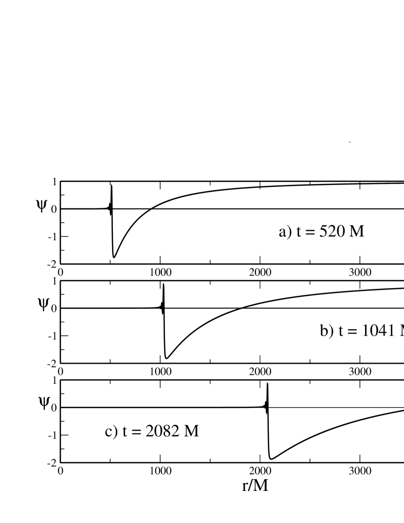
Figure 1: The evolution of initial data of the form $\{\psi(t=0,r)=1,\psi_{t}(t=0,r)=0\}$, at times $t=520M$, (plot a)), $t=1041M$, (plot b)) and $t=2082M$, (plot c)). The quasinormal ringing, noticeable as a structure near $r=500M$, $r=1000M$, and $r=2000M$, respectively in a), b) and c) is shown enlarged in Figure 2, a), for $t=520M$. Notice that the point where $\psi$ first changes sign moves to the right at about twice the speed of the quasinormal ringing, as indicated in the text

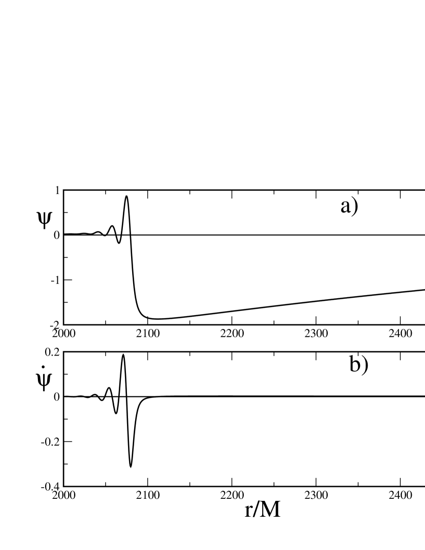
Figure 2: The region where the wave form is dominated by quasinormal ringing, at $t=520M$, is indicated for $\psi$ in a), and for $\partial\psi/\partial t$ in b)

Putting these results together, we expect that after some time $t_{0}$ of evolution of our initial data, we should see an essentially vanishing wave form up to $r\simeq t_{0}$, where we should see some quasinormal ringing type wave form, followed by a region where $\psi$ slowly changes sign and finally approaches the constant asymptotic value of the initial data. This is indeed what happens if we numerically integrate the Zerilli equation. In Figure 1 we indicate the results of evolving initial data of the form $\psi(r_{*},t=0)=1$, $\partial_{t}\psi(r_{*},t=0)=0$, form $M=1$, through several times. Curve a) corresponds to $t=520M$, curve b) to $t=1041M$, and c) to $t=2082M$. A detail of the quasinormal ringing part, for $t=510M$, is included in Figure 2, a), while Figure 2, b) displays the time derivative of $\psi$. It can be seen that these results display all the expected features. In particular, we find a form of “gravitational memory effect”, since at large distances from the black hole, the gravitational wave amplitude $\psi$ starts with a certain non vanishing constant value and goes to a different constant value (in this case zero), after some quasi-normal ringing signal is observed. We discuss this effect in more detail in the next Section.

VI Final comments and conclusions

The results obtained in the previous Section indicate the existence of a certain gravitational memory effect associated to a particular type of initial data, for instance, that obtained for single boosted black holes using the Bowen - York Ansatz BoYo . We may picture what this implies by considering its effect on an interferometric type detector of gravitational waves, placed at a large distance from the black hole, that is turned on at $t=0$. There one finds a very slow drift of the equilibrium position, followed by the quasi-normal ringing signal, with the interferometer ending up in an equilibrium position that is shifted with respect to the initial one, in an effect that holds certain similarity to the well known “gravitational memory” effect christo ; thorne ; blanchet . In fact, this is closer to the type of effect originally envisioned by Grischuk, et.al. grischuk , while its relation to the Christodoulou christo type of gravitational memory is unclear to us, although we remark that the nonlinear nature of the Einstein equations is involved, since we had to consider second order gauge transformations to arrive at our final result.

It is well known that the initial data constructed in accordance with the conformal flatness prescription has the physical drawback that it generally implies incoming gravitational radiation in the past. For binary black hole collisions, such as in the Misner misner initial data or, more generally, for boosted black hole data as considered in boosted , this seems to introduce no particular undesirable or unexpected features, at least in the close limit approximation in center of momentum frame. For a perturbed single boosted black hole, however, we find that the conformal flatness of the initial data introduces a new type of gravitational memory effect that we would expect to be absent in the absence of incoming gravitational radiation. Going back to the original problem of the “appropriate” asymptotic behavior of the initial data for a perturbed boosted single black hole, we may conclude that the “natural” choice that would be physically expected in the absence of substantial incoming radiation, should lead in the boosted frame where the momentum is $P$, to a Zerilli function that approaches the constant value $\psi\rightarrow(2/3)P^{2}/M$ for large $r$ , in agreement with the discussion carried out in this Paper.

Finally, our results can also be considered in relation with analyses such those of Kennefick kennefick , applied, for instance, to a system such as a black hole surrounded by a spherically symmetric stationary mass distribution, that eventually collapses in an asymmetrical manner, inducing a recoil of the final black hole, together with the emission of gravitational radiation. In accordance with our analysis, far away from the source, we have initially a stationary Schwarzschild spacetime, where $\psi$ vanishes, but, after the passage of the gravitational radiation associated to the collapse, the spacetime should correspond to a “boosted” Schwarzschild, where $\psi$ is a non vanishing constant, exactly as envisioned in kennefick . Notice that the final value of $\psi$ is related to the recoil momentum as derived in Section XX, and this in turn is related to the anisotropy of the emmited radiation, so that we seem to have a further interpretation for the Cristodoulou type of gravitational memory.

Appendix A A boosted Schwarzschild metric

Consider the Schwarzschild metric, written in the form

$$ds^{2}=-(1-2M/r)dt^{2}+(1-2M/r)^{-1}dr^{2}+r^{2}[d\theta^{2}+\sin^{2}\theta d\phi^{2}]$$ (31)

We consider (31) only for $r>2M$, and all $t$. In that region, we may consider, instead of $t,r,\theta,\phi$, new coordinates $t^{\prime},r^{\prime},\theta^{\prime},\phi^{\prime}$, related to the old ones by

$$\phi = \phi^{\prime}$$

$$\theta = \theta^{\prime}-(vt^{\prime}/r^{\prime})\sin(\theta^{\prime})$$

$$r = r^{\prime}-vt^{\prime}\cos(\theta^{\prime})$$

$$t = t^{\prime}-vr^{\prime}\cos(\theta^{\prime})$$ (32)

This coordinate transformation is motivated by considering a Lorentz boost along the positive $z$-axis, with velocity $v$, of an auxiliary coordinate system $t,x,y,z$, related to $t,r,\theta,\phi$ as flat cartesian coordinates to the corresponding Schwarzschild spherical polar coordinates, and keeping only terms of order $v$, but this is not central to our discussion. The transformation (A) can be used to write the Schwarzschild metric in $t^{\prime},r^{\prime},\theta^{\prime},\phi^{\prime}$, coordinates. The resulting expression for the line element is rather long and we shall not display it here. The important point is that it is diffeomorphic to (31), and the metric components are smooth functions of $v$ near $v=0$, with (31) recovered for $v=0$. If we expand the metric coefficients in powers of $v$, we find that to order $v$ the metric is asymptotically flat in the sense used in Section IV. We may use (18) to compute $P$. The result is $P=vM$, which corresponds to the relativistic momentum of an object of (rest) mass $M$, computed to order $v$. If we consider now the expansion to order $v^{2}$, we find that the metric is not asymptotically flat to that order, again in agreement with Section IV. We may now consider a new coordinate transformation, of order $v^{2}$, to restores the asymptotic flatness, but, since the Zerilli function is invariant under this transformation, we may use the results obtained already in $t^{\prime},r^{\prime},\theta^{\prime},\phi^{\prime}$ coordinates to compute it. The result is,

$$\psi_{B}(t^{\prime}=0,r^{\prime})={4v^{2}M(r^{\prime}-2M)(3r^{\prime}+2M)\over 9r^{\prime}(2r^{\prime}+3M)}\simeq-{2\over 3}Mv^{2}+{\cal{O}}(1/r^{\prime})$$ (33)

which displays the expect asymptotic constant value for $\psi_{B}\simeq 2P^{2}/(3M)$.

References

- (1) R. H. Price and J. Pullin, Phys. Rev. Lett. 72 (1994) 3297 .
- (2) For a recent review, see, e.g., J. Pullin, Prog.Theor.Phys.Suppl. 136 (1999) 107-120
- (3) T. Regge, J. Wheeler, Phys. Rev. 108 (1957) 1063.
- (4) F. J. Zerilli, Phys. Rev. D2 (1970) 2141.
- (5) R. J. Gleiser, C. Nicasio, R. H. Price, J. Pullin, Phys.Rept. 325 (2000) 41-81
- (6) V. Moncrief, Ann. Phys. (NY) 88 (1974) 323.
- (7) R. J. Gleiser, G. Khanna, J. Pullin, Phys.Rev. D66 (2002) 024035
- (8) M. Bruni, S. Matarrese, S. Mollerach, S. Sonego, Class.Quant.Grav. 14 (1997) 2585-2606
- (9) R. H. Price, Phys. Rev. D5 (1972) 2419.
- (10) B.S. Kay and R.M. Wald, Class.Quant.Grav.4 (1987) 893
- (11) J. M. Bowen, J. W. York, Phys. Rev. D21, 2047 (1980).
- (12) D. Christodoulou, Phys. Rev. Lett. 67 (1991) 1486.
- (13) K.S. Thorne, Phys.Rev. D45 (1992) 520.
- (14) L. Blanchet and T. Damour, Phys.Rev. D46 (1992) 4304.
- (15) V. B. Braginsky and L. P. Grischuk, Zh. Eksp. Teor. Fiz. bf 89(1985) 744 [Sov.Phys. JETP 62 (1985) 427]
- (16) C. Misner, Phys. Rev. 118 (1960) 1110.
- (17) C. O. Nicasio, R. J. Gleiser, R. H. Price, J. Pullin, Phys.Rev. D59 (1999) 044024.
- (18) D. Kennefick, Phys. Rev. D50 (1994) 3587.