Gravitational decoherence

Abstract

We investigate the effect of quantum metric fluctuations on qubits that are gravitationally coupled to a background spacetime. In our first example, we study the propagation of a qubit in flat spacetime whose metric is subject to flat quantum fluctuations with a Gaussian spectrum. We find that these fluctuations cause two changes in the state of the qubit: they lead to a phase drift, as well as the expected exponential suppression (decoherence) of the off-diagonal terms in the density matrix. Secondly, we calculate the decoherence of a qubit in a circular orbit around a Schwarzschild black hole. The no-hair theorems suggest a quantum state for the metric in which the black hole’s mass fluctuates with a thermal spectrum at the Hawking temperature. Again, we find that the orbiting qubit undergoes decoherence and a phase drift that both depend on the temperature of the black hole. Thirdly, we study the interaction of coherent and squeezed gravitational waves with a qubit in uniform motion. Finally, we investigate the decoherence of an accelerating qubit in Minkowski spacetime due to the Unruh effect. In this case decoherence is not due to fluctuations in the metric, but instead is caused by coupling (which we model with a standard Hamiltonian) between the qubit and the thermal cloud of Unruh particles bathing it. When the accelerating qubit is entangled with a stationary partner, the decoherence should induce a corresponding loss in teleportation fidelity.

I Introduction

For much of its history, experimental observation of quantum gravitational effects has been little more than an impossible dream for general relativity. Yet recent theoretical developments have begun to alter this view. New ideas in quantum gravity, including string theory, are being explored, which, if correct, would imply the presence of quantum gravitational behavior at length scales much larger than Planckian BHfactories ; Jacobson ; Yurtholo . Combined with emerging sensor and other technologies, these speculations are raising the specter of near-term experimental tests for some of the most fundamental manifestations of quantum spacetime structure.

An imperfect but illuminating analogy can be pursued in the physics of fluids. Consider a hypothetical stage in the development of the theory of fluids in which we are unaware of the atomic structure of matter, while we understand the Navier-Stokes equations and are somehow aware of Planck’s constant, $\hbar$. In this analogy, the atomic structure of fluids is the unknown holy grail of quantum fluid mechanics which we are striving to discover with our limited knowledge. The fundamental quantities characterizing a fluid classically can be taken to be the speed of sound, $c_{s}$, and the density, $\rho$. Along with $\hbar$, these quantities can be combined to define a length scale

$$l_{q}=\left(\frac{\hbar}{\rho\,c_{s}}\right)^{\!\!\frac{1}{4}}$$ (1)

which would seem to set the quantum regime where classical fluid mechanics must break down. For typical fluids (e.g. water), $l_{q}$ is of order $10^{-8}\,\mbox{cm}$; it does a remarkably good job of predicting the atomic scale. But in our hypothetical ignorance of atoms, we would be ill-advised to conclude that quantum effects must be negligible all the way down to the length scale $l_{q}$. Indeed, we know (in hindsight) from kinetic theory that the true length scale which sets the breakdown of classical fluid mechanics is the correlation length, which is typically much larger than $l_{q}$. Collective phenomena such as phase transitions may give rise to correlation lengths that are macroscopically large. Even away from phase transitions, correlation lengths are large enough to have effects (such as Brownian motion) that are readily observable in experiments performed far above the lengthscale $l_{q}$.

What this analogy teaches us is to be open to the possibility that, while the Planck length sets the scale for quantum gravity, there may be quantum effects of the unknown small-scale structure of spacetime which are analogous to phase transitions or Brownian motion, and which might be detectable at scales far above Planck. In this paper we will explore one possible source for such effects: quantum fluctuations in a background spacetime causing decoherence in qubits kinematically coupled to that background. In a sense, such decoherence would be analogous to Brownian motion caused by the small-scale structure of a fluid. We will make very few assumptions about the quantum theory of spacetime underlying the fluctuations, apart from demanding that it results in a Hilbert space structure for states of the metric which obeys the standard laws of quantum mechanics. We will conclude the paper by discussing a slightly different scenario for gravitational decoherence: the decoherence of an accelerating qubit in Minkowski spacetime due to the Unruh effect. In this case decoherence is not due to fluctuations in the metric, but instead is caused by a coupling (which we model with a standard Hamiltonian) between the qubit and the thermal cloud of Unruh particles bathing it.

A separate set of motivations for studying gravitational decoherence arises from relativistic quantum information theory, a new field of research that studies the properties of quantum information and quantum communication as seen by observers in moving frames. One of the most important ingredients of quantum information theory is entanglement, and much of the interest so far has been directed to its properties under Lorentz transformations. Czachor studied a version of the EPR experiment with relativistic particles czachor97 , and Peres et al. demonstrated that the spin of an electron is not covariant under Lorentz transformations peres02 . Furthermore, the effect of Lorentz transformations on maximally spin-entangled Bell states in momentum eigenstates was studied by Alsing and Milburn alsing02 , and Gingrich and Adami derived the general transformation rules for the spin-momentum entanglement of two qubits gingrich02 . Recently, these results were extended to the Lorentz transformation of polarization entanglement gingrich03 , and to situations where one observer is accelerated alsing03 . Here, we take a look at a different aspect of relativistic quantum information theory: the effect of decoherence on a qubit due to quantum fluctuations in the metric.

We will now turn our attention to the study of decoherence in the four major paradigms of relativity: First, we will calculate the effect of flat fluctuations in the fabric of Minkowski spacetime on a linearly moving qubit. Next, we put a qubit in orbit around a black hole. The mass fluctuations due to the Hawking radiation induce fluctuations in the Schwarzschild metric, which in turn couple to our qubit. Following black holes, we will study the interaction of a linearly moving qubit with coherent and squeezed gravity waves. Coherent states correspond to classical gravitational waves which are expected to arise from astrophysical processes such as the inspiral of compact binaries, while squeezing arises due to the expansion of the universe. Finally, we study a related but qualitatively different decoherence phenomenon: we derive the decoherence of a linearly accelerating qubit in a bath of Unruh radiation. This treatment requires a field-theoretical description of the thermal Unruh bath, while we will be content with a first-quantized description of the qubit, whose interaction with the quantum field of Unruh particles we will model with a standard Hamiltonian.

First, we define a general quantum system to be in a state $|\psi\rangle=\sum_{k}c_{k}|k\rangle$, where $\{|k\rangle\}_{k}$ is a complete set of (non-degenerate and discrete) eigenstates of the Hamiltonian. The free evolution of $|\psi\rangle$ is given by

$$|\psi(t)\rangle=\sum_{k}c_{k}e^{iE_{k}t/\hbar}|k\rangle\equiv\sum_{k}c_{k}e^{i\omega_{k}t}|k\rangle\;.$$ (2)

We consider the situation where the quantum system moves along a geodesic path in some fixed metric $g_{0}$, while the true metric $g$ is subject to quantum fluctuations about $g_{0}$. The proper time of the system is denoted by $\tau$, and we have $|\psi(\tau)\rangle=\sum_{k}c_{k}e^{i\omega_{k}\tau}|k\rangle$. The laboratory coordinates are $t$, $x$, $y$, and $z$. We want to know the state of the quantum system $|\psi(t)\rangle$ in laboratory coordinates. This depends on the metric $g$:

$$ds^{2}=g_{\mu\nu}\,dx^{\mu}dx^{\nu}=d\tau^{2}\;,$$ (3)

where the last equality follows from the geodesic motion of the quantum system.

Now suppose that the metric itself is a (highly delocalized) quantum system in a state $\rho_{g}$. It is our central assumption that this quantum metric behaves as a regular quantum system. In particular, we assume that the superposition principle is valid for quantum states of the metric. We initialize the state of our quantum system at time $t=0$ in $|\psi(0)\rangle=\sum_{k}c_{k}|k\rangle$, and let it evolve freely within the metric $\rho_{G}$ for a certain period. The state of the system will generally become entangled with the metric, and we wish to determine the reduced density matrix of the system at time $t$.

In general, the free evolution of an energy eigenstate $|k\rangle$ in a particular quantum metric $|g_{j}\rangle$ is given by

$$|k\rangle|g_{j}\rangle\rightarrow e^{i\omega_{k}\tau_{j}}|k\rangle|g_{j}\rangle\;,$$ (4)

with $d\tau=dt\sqrt{g_{\mu\nu}\,\dot{x}^{\mu}\,\dot{x}^{\nu}}$, and $\dot{x}^{\mu}\equiv dx^{\mu}/dt$. There is no back-action of the state of the qubit onto the metric. Specifying the (fluctuating) quantum metric and the geodesic motion of the quantum system allows us to determine the reduced density matrix of the quantum system.

Rather than the general state in Eq. (2), we consider a qubit in a state

$$|\psi\rangle=\frac{1}{\sqrt{2}}\left(|0\rangle+e^{i\varphi}|1\rangle\right)\;.$$ (5)

We could have chosen a more general state with differing relative amplitudes, but it turns out that this state gives rise to all the interesting physical features of the interaction model we study here. Similarly, the general case of an $N$-level system does not give rise to conceptually new physics.

Next, we will consider the geodesic motion of a qubit in three different fluctuating quantum spacetime metrics. We consider “flat” fluctuations in a two-dimensional Minkowski space in Sec. II, mass fluctuations in the Schwarzschild metric for circular orbits of the qubit in Sec. III, and graviton-number fluctuations in coherent and squeezed gravity waves in Sec. IV.

II Fluctuations in flat spacetime

In this section we calculate the density matrix of a qubit that experiences decoherence due to “flat” fluctuations in the Minkowski spacetime metric.

II.1 The Minkowski metric

First, consider a uniformly moving qubit with velocity $dx/dt=v$ in the $x$-direction in a two-dimensional flat Minkowski space. Let the state of the metric be given by

$$\rho_{g}=\int d\vec{a}\,f(\vec{a})\,|g_{\vec{a}}\rangle\langle g_{\vec{a}}|\;,$$ (6)

with $\vec{a}=(a_{1},a_{2},a_{3},a_{4})\in\mathbb{R}^{4}$ and $g_{\vec{a}}$ a particular metric given by

$$g_{\vec{a}}=\begin{pmatrix}a_{1}+1&a_{2}\cr a_{3}&a_{4}+1\end{pmatrix}\begin{pmatrix}-1&0\cr 0&1\end{pmatrix}\begin{pmatrix}a_{1}+1&a_{3}\cr a_{2}&a_{4}+1\end{pmatrix}.$$ (7)

This defines the “flat” fluctuations in the two-dimensional Minkowski space. The distribution function $f(\vec{a})$ determines the quantum fluctuations of the metric around $\vec{a}=0$. We assume that the fluctuations are Gaussian:

$$f(\vec{a})=\exp\left(-\sum_{jk=1}^{4}a_{j}A_{jk}a_{k}\right)\equiv\exp\left[-(\vec{a},A\vec{a})\right]\;,$$ (8)

where $A$ is a positive symmetric variance matrix. The (dimensionless) parameters specified by the matrix elements of $A$ would ideally be derived from a complete quantum theory of gravity. In the absence of such a theory, we would treat the $A_{ij}$ as arbitrary real parameters.

The proper time $\tau$ of the qubit in motion, given a particular metric $g_{\vec{a}}$, is given by

$$d\tau=dt\sqrt{g_{00}+2g_{0x}\,v+g_{xx}\,v^{2}}\;,$$ (9)

where

$$g_{00} = a_{1}^{2}-a_{2}^{2}+2a_{1}+1$$ (10a)

$$g_{0x} = a_{1}a_{3}-a_{2}a_{4}+a_{3}-a_{2}$$ (10b)

$$g_{xx} = a_{3}^{2}-a_{4}^{2}-2a_{4}-1\;.$$ (10c)

Furthermore, we assume linear motion, yielding $dx=v\,dt$, with $\hbar=c=G=1$. In the following, we will use $\Omega\equiv\omega_{1}-\omega_{0}$.

II.2 The decoherence model

The procedure to calculate the decoherence due to the above interaction of the qubit with the metric is as follows: first we write the total state $\rho=|\psi\rangle\langle\psi|\otimes\rho_{g}$, and we apply the interaction from Eq. (4). We then substitute the expression from Eq. (9) into the resulting state. In fact we will use the polynomial expansion of the square root to second order. This is justified since the fluctuations are small. Subsequently, we trace out the metric state, since we have no direct access to its fluctuations. We can then evaluate the integral in Eq. (6), which yields an expression for the reduced density matrix of the qubit.

The joint system of the qubit and the metric after the interaction of Eq. (4) is in the state

$$\rho = \int_{{\mathbb{R}}^{4}}d\vec{a}\,e^{-(\vec{a},A\vec{a})}\left[|0\rangle\langle 0|+e^{-i(\varphi+\Omega\tau)}|0\rangle\langle 1|\right.$$ (12)

$$\qquad\qquad\left.+e^{i(\varphi+\Omega\tau)}|1\rangle\langle 0|+|1\rangle\langle 1|\right]\;.$$

Substituting Eq. (9) into the above expression and expanding to second order will yield a state $\alpha|0\rangle\langle 0|+e^{-i\varphi}\beta^{*}|0\rangle\langle 1|+e^{i\varphi}\beta|1\rangle\langle 0|+\alpha|1\rangle\langle 1|$, with

$$\alpha=\int_{{\mathbb{R}}^{4}}d\vec{a}\,e^{-(\vec{a},A\vec{a})}=\frac{\pi^{2}}{\sqrt{\det A}}\;,$$ (13)

and

$$\beta=\int_{{\mathbb{R}}^{4}}d\vec{a}\,e^{-(\vec{a},A\vec{a})+i\Omega\tau(\vec{a})}\;.$$ (14)

The proper time $\tau(\vec{a})$ is approximated by

$$\tau(\vec{a})=t\left[c_{0}+(\vec{c}_{1},\vec{a})+(\vec{a},C_{2}\vec{a})+O(\vec{a}^{3})\right]\;,$$ (15)

with

$$c_{0}(v) = 1-\frac{v^{2}}{2}-\frac{v^{4}}{8}+\ldots=\sqrt{1-v^{2}}\equiv\gamma$$ (16a)

$$\vec{c}_{1}(v) = \left(1-\frac{v^{2}}{2}\right)(1,-v,v,-v^{2})$$ (16b)

$$C_{2}(v) = \frac{1}{2}\begin{pmatrix}\frac{v^{2}}{2}&v&\frac{v^{3}}{2}&v^{2}\cr v&1-\frac{3v^{2}}{2}&v^{2}&-v-\frac{3v^{3}}{2}\cr\frac{v^{3}}{2}&v^{2}&\frac{v^{4}}{2}&v^{3}\cr v^{2}&-v-\frac{3v^{3}}{2}&v^{3}&-v^{2}-\frac{3v^{4}}{2}\cr\end{pmatrix}.$$ (16c)

In order to calculate $\beta$, we collect all the second-order terms $a_{j}a_{k}$ into the variance matrix $A$ (yielding a new positive symmetric matrix $B=A+i\Omega t\,C_{2}$), and the first-order terms are collected in a linear exponential:

$$\beta=e^{i\Omega t\gamma}\int_{{\mathbb{R}}^{4}}d\vec{a}\,e^{-(\vec{a},B\vec{a})+(\vec{u},\vec{a})}\;,$$ (17)

where $\vec{u}=i\Omega t(1+v^{2}/2)(1,-v,v,-v^{2})$. The overall phase factor originates from the time dilation observed for a moving body with velocity $v$. The integral in Eq. (17) can be evaluated formally to yield

$$\int_{{\mathbb{R}}^{4}}d\vec{a}\,e^{-(\vec{a},B\vec{a})+(\vec{u},\vec{a})}=\frac{\pi^{2}e^{(\vec{u},B^{-1}\vec{u})}}{\sqrt{\det B}}\;.$$ (18)

For the integral to exist, the real part of the eigenvalues of $B$ must be strictly positive, which is ensured by $A$.

Given a particular variance matrix $A$, we can calculate the (normalized) state of the qubit as a function of the travelled coordinate time $t$:

$$\rho(t)=\frac{1}{2}\begin{pmatrix}1&\eta\,e^{i(\varphi^{\prime}+\delta)}e^{-\Gamma^{2}}\cr\eta\,e^{-i(\varphi^{\prime}+\delta)}e^{-\Gamma^{2}}&1\end{pmatrix}\;,$$ (19)

where $\varphi^{\prime}=\varphi+\gamma\Omega t$ is the time-dilated free evolution of the qubit, and $\eta\equiv\sqrt{\det A/\det B}$. Furthermore, we defined

$$\Gamma^{2}\equiv\mbox{\rm Re}[-(\vec{u},B^{-1}\vec{u})]\quad\text{and}\quad\delta\equiv\mbox{\rm Im}[-(\vec{u},B^{-1}\vec{u})]\;.$$ (20)

When the variance matrix is diagonal ($A=\sigma^{-2}\mbox{\small 1}\!\!\mbox{1}$), i.e., when there are no special correlations between the different space-time dimensions, we can give a fairly straightforward expression of the decohered qubit. Since the quantum fluctuations of the metric are assumed small (Planck scale), the variance $\sigma$ is small, and we can expand the solution around $\sigma=0$. Using Mathematica, we find that

$$\Gamma=(1+v^{2})\,\Omega t\,\sigma\;,$$ (21)

and

$$\delta=\frac{1}{4}v^{2}(5+5v^{2}+11v^{4}+3v^{6})\,\Omega^{3}t^{3}\sigma^{4}\;.$$ (22)

Interestingly, there are three effects that alter the state of the qubit. First, there is the expected decoherence $\exp(-\Gamma^{2})$, the argument of which scales quadratically with time $t$, frequency difference $\Omega$, and variance $\sigma$. Secondly, we found a phase drift $\delta$, due to the interaction with the quantum metric. This effect scales with $(\Omega t)^{3}$ and $\sigma^{4}$, and it arises when there are off-diagonal terms in the matrix $B$, or, equivalently, when there are $a_{j}a_{k}$ terms with $j\neq k$ in Eq. (15). Finally the factor $\eta$ behaves according to

$$\eta=\sqrt{\frac{\det A}{\det B}}\propto 1+\frac{i}{2}(1+v^{2})^{2}\Omega t\sigma^{2}\;.$$ (23)

The evolution of the complex off-diagonal element is shown in Fig. 1.

Figure 1: The amplitude and phase of the off-diagonal element of the density matrix. The inward spiralling is due to the phase drift and the decoherence. The knee in the figure around the point $(\mbox{\rm Re},\mbox{\rm Im})=(0.8,0.1)$ is due to the complex factor $\eta$.

The interaction of the quantum fluctuations of the metric with a qubit generalizes directly to the case of an $N$-level system, or quNit. The density matrix will be an $N\times N$ matrix, and the off-diagonal elements will be of the form $\eta\,e^{i(\varphi_{jk}^{\prime}+\delta_{jk})}e^{-\Gamma_{jk}}$. We obtain $\varphi_{jk}^{\prime}$, $\delta_{jk}$, and $\Gamma_{jk}$ from Eqs. (19), (21) and (22) by substituting $\Omega_{jk}\equiv\omega_{j}-\omega_{k}$ for $\Omega$.

II.3 Ensemble of qubits

Note that the above calculation describes an experiment in which the ensemble of qubits necessary to statistically measure the reduced quantum state of the qubit is obtained via repetition of each ensemble qubit’s time evolution through the same metric state Eq. 6. What happens when we send an ensemble of $N$ qubits with uniform velocity $v$, while their states are all subjected to the same fluctuations in the Minkowski metric simultaneously? Let $|s\rangle$ be an $N$-bit string, and $0\leq n(s)\leq N$ the number of ones in $|s\rangle$. The evolution of a bit string $|s\rangle$ on the metric $|g_{\vec{a}}\rangle$ in terms of the proper time $\tau$ is given by

$$|s\rangle|g_{\vec{a}}\rangle~{}\rightarrow~{}\exp[i\,n(s)\,\Omega\tau_{\vec{a}}]|s\rangle|g_{\vec{a}}\rangle\;.$$ (24)

There are $2^{N}$ such strings, comprising a set ${\mathcal{S}}$, and the density operator becomes a $2^{N}\times 2^{N}$ matrix:

$$\rho_{N}=\int_{{\mathbb{R}}^{4}}d\vec{a}\,e^{-(\vec{a},A\vec{a})}\left[\sum_{s,s^{\prime}}e^{i[n(s)-n(s^{\prime})\Omega t]}|s\rangle\langle s^{\prime}|\right]\;.$$ (25)

It is immediately obvious that the states most sensitive to this type of decoherence is the maximally entangled GHZ state $|00\ldots 0\rangle+|11\ldots 1\rangle$, that is, states that have maximal $n(s)-n(s^{\prime})$. As a direct consequence, these states can in principle be used to detect the fluctuations lee02 .

Similarly, it is now also clear that such decoherence can be countered by encoding quantum information in the decoherence-free subspace spanned by the subsets of ${\mathcal{S}}$ for which $n(s)-n(s^{\prime})=0$. For a given $n(s)$, there are $\binom{N}{n(s)}$ such states. This behaviour is reminiscent of the technique used in Ref. bartlett03 .

III Mass fluctuations in black holes

III.1 The Schwarzschild metric

Now, we will turn our attention to the situation of a qubit orbiting a black hole, and we again assume that the metric is a quantum mechanical object. The no-hair theorems for black-hole structure suggest that quantum fluctuations in the metric will consist of fluctuations in the mass of the black hole (hence we neglect the fluctuations in angular momentum, and assume that charge fluctuations are forbidden in quantum gravity because of super-selection rules).

For simplicity, we assume that the orbit of the qubit is circular. The Schwarzschild metric of a given mass $M$ is given by

$$ds^{2}=g_{M}\equiv-\left(1-\frac{2M}{r}\right)dt^{2}+\frac{dr^{2}}{1-\frac{2M}{r}}+r^{2}d\Omega^{2}\;,$$ (26)

where $d\Omega^{2}\equiv d\theta^{2}+\sin^{2}\theta\,d\phi^{2}$.

The evolution of energy eigenstates is again given by Eq. (4). We need to express $\tau$ in terms of $t$. To this end, we start from the Hamiltonian for geodesic motion in the Schwarzschild background

$$H = \frac{1}{2}g^{\mu\nu}p_{\mu}p_{\nu}$$ (27)

$$= -\frac{p_{0}^{2}}{2-\frac{4M}{r}}+\left(1-\frac{2M}{r}\right)\frac{p_{r}^{2}}{2}+\frac{p_{\theta}^{2}}{2r^{2}}+\frac{p_{\phi}^{2}}{2r^{2}\sin^{2}\theta}$$ (28)

$$= -\frac{E^{2}}{2\left(1-\frac{2M}{r}\right)}+\frac{1}{2}\left(1-\frac{2M}{r}\right)p_{r}^{2}+\frac{L^{2}}{2r^{2}}$$ (29)

$$= -\frac{1}{2}\;.$$ (30)

Here we have assumed without loss of generality that the orbital plane has $\theta=\pi/2$ and thus by spherical symmetry $p_{\theta}=0$. Furthermore, we introduced the energy $E=-p_{0}$ and the angular momentum $L=p_{\phi}$. The last equality holds since the four-velocity $v=dx/d\tau$ is normalized: $v^{\mu}v_{\mu}=g^{\mu\nu}p_{\mu}p_{\nu}=-1$. Furthermore, we have

$$p_{0}=g_{00}v^{0}=-\left(1-\frac{2M}{r}\right)\frac{dt}{d\tau}=-E\;,$$ (31)

which gives us an expression for $\tau$ in terms of $t$ and $E$. We now need to determine $E$.

¿From Eq. (27) and $p_{r}=0$ (since we consider a circular orbit), we derive

$$E^{2}=\left(1-\frac{2M}{r}\right)\left(1+\frac{L^{2}}{r^{2}}\right)\equiv V(r)\;.$$ (32)

For stable orbits we need the potential $V(r)$ to be a minimum:

$$\left.\frac{\partial V}{\partial r}\right|_{r_{0}}=0\quad\text{and}\quad\left.\frac{\partial^{2}V}{\partial r^{2}}\right|_{r_{0}}>0\;.$$ (33)

This yields

$$\left(1-\frac{2M}{r_{0}}\right)\frac{L^{2}}{r^{3}_{0}}-\frac{M}{r^{2}_{0}}\left(1+\frac{L^{2}}{r^{2}_{0}}\right)=0\;,$$ (34)

or

$$L^{2}=\frac{Mr_{0}^{2}}{r_{0}-3M}\;$$ (35)

which makes manifest the well-known fact that there are no stable circular orbits inside the critical radius $r=3M$. For any $r_{0}>3M$, a circular orbit at $r=r_{0}$ can be found with the above value of $L$. On such an orbit, the energy $E$ is determined by substituting $L^{2}$ into $V(r_{0})$; from Eq. (27) we find that

$$d\tau^{2}=\left(1-\frac{3M}{r_{0}}\right)dt^{2}\;.$$ (36)

We will assume that the black hole is in thermal equilibrium with the thermal Hawking radiation it emits at the temperature $T_{H}$. This is equivalent to assuming that the black hole is inside a conducting sphere with perfectly reflecting walls placed at a large radius away from the horizon. The quantum state of the metric can then be written as in Eq. (6) in the form

$$\rho_{g}=\int dM\,\exp\left[-\frac{(M-M_{0})^{2}}{2\sigma_{M}^{2}}\right]|g_{M}\rangle\langle g_{M}|\;,$$ (37)

where $M_{0}$ denotes the classical mass of the hole, about which the mass $M$ fluctuates in equilibrium with the thermal bath at temperature $T_{H}$. The fluctuations are Gaussian (in accordance with the thermodynamic limit) around $M_{0}$. More precisely, a general canonical ensemble with Hamiltonian $H$ has energy fluctuations given by

$$\langle H^{2}\rangle-\langle H\rangle^{2}=\frac{\partial^{2}}{\partial\beta^{2}}\log Z=-\frac{\partial}{\partial\beta}\langle H\rangle\;,$$ (38)

where $Z=\int e^{-\beta H}$ is the partition function, $\beta=1/(k_{B}T)$ is the inverse temperature, and $\langle\cdots\rangle$ denotes the canonical ensemble average; thus, e.g., $\langle H\rangle$ is equal to the internal energy $U$. According to our assumption as explained below, $\sigma^{2}_{M}$ will be given by

$$\sigma_{M}^{2}=\langle H^{2}\rangle_{T_{H}}-\langle H{\rangle^{2}}_{T_{H}}\;,$$ (39)

i.e. equal to the energy fluctuations of a Bose gas at thermal equilibrium with black-body radiation at the Hawking temperature.

In order to find the effect of thermal fluctuations in the black-hole mass on the evolution of coherence in the state of our qubit in circular orbit at $r=r_{0}$, we calculate the off-diagonal element of the qubit’s density matrix:

$$\beta = \int_{-\infty}^{+\infty}dM\,\exp\left[-\frac{(M-M_{0})^{2}}{2\sigma^{2}_{M}}\right]e^{i\Omega t\sqrt{1-\frac{3M}{r_{0}}}}$$ (40)

$$= \sqrt{\frac{9M_{0}^{2}\Omega t}{8r_{0}^{2}+18i(\Omega)^{2}t\sigma_{M}^{2}}}\;\exp\left(-\Gamma^{2}+i\delta\right)\;,$$ (41)

where

$$\Gamma=\frac{9\sqrt{2}}{8}\left(\frac{3M_{0}+2r_{0}}{r_{0}^{2}}\right)\Omega t\,\sigma_{M}\;,$$ (42)

and

$$\delta = \Omega t\sqrt{1-\frac{3M_{0}}{r_{0}}}$$ (44)

$$\qquad+\frac{81}{128}\left(\frac{3M_{0}+2r_{0}}{r_{0}^{6}}\right)^{2}\Omega^{3}t^{3}\,\sigma_{M}^{4}\;.$$

The first term of the phase drift is the regular relativistic effect, and the second term is the variational phase drift due to the quantum fluctuations in the mass of the black hole. The off-diagonal element of the density matrix evolves similar to the one in the previous section (see Fig. 1).

III.2 Mass fluctuations

Now we seek an expression for $\sigma_{M}$. We know that the Hawking temperature of a black hole is proportional to the surface gravity $\kappa$ wald94 :

$$kT_{H}=\frac{\hbar}{c}\frac{\kappa}{2\pi}=\frac{\hbar c^{3}}{8\pi GM}\;,$$ (45)

where we have used the fact that a non-rotating neutral black hole of mass $M$ has $\kappa=(4GM/c^{4})^{-1}$, and therefore ${\beta}^{-1}=kT_{H}=\hbar c^{3}/(8\pi GM)$ wald84 . For clarity we will keep the physical constants $\hbar$, $c$ and $G$ in arbitrary units throughout this subsection.

The Hawking radiation has a perfect black-body spectrum. We will assume that the fluctuations in the mass of the hole are identical to the fluctuations in the average energy $U$ of a black body of surface area $4\pi G^{2}{M_{0}}^{2}/c^{4}$ (the area of the black-hole horizon) radiating at the Hawking temperature $T_{H}$. The average internal energy of a black body (Boson gas) of volume $V$ at temperature $T$ is given by

$$\langle H\rangle=U=\frac{4\sigma}{c}\,V\,T^{4}=\frac{\pi^{2}{k_{B}}^{4}}{15\hbar^{3}c^{3}}V\,T^{4}=\frac{\pi^{2}}{15\hbar^{3}c^{3}}\frac{V}{\beta^{4}}\;,$$ (46)

where $\sigma$ is the Stefan-Boltzmann constant. According to Eqs. (34)–(35)

$$c^{4}\;\sigma_{M}^{2}=\langle H^{2}\rangle-\langle H\rangle^{2}=\frac{4\pi^{2}}{15\hbar^{3}c^{3}}\frac{V}{\beta^{5}}\;.$$ (47)

Note that the black-body energy $U$ itself is not equal to the classical hole mass $M_{0}$; it is only the mean-square fluctuations $\sigma_{M}^{2}$ about $M_{0}$ that we assume are identical to the thermal fluctuations in $U$ at the Hawking temperature. Substituting the Hawking value $\beta=8\pi GM_{0}/(\hbar c^{3})$, and the geometric identity $V=(32\pi/3)G^{3}{M_{0}}^{3}/c^{6}$ in Eq. (41), we finally obtain

$$\sigma_{M}^{2}=\frac{\hbar^{2}c^{2}}{11520\,\pi^{2}G^{2}}\frac{1}{{M_{0}}^{2}}=\frac{{m_{p}}^{2}}{11520\,\pi^{2}}\left(\frac{m_{p}}{M_{0}}\right)^{2}\;,$$ (48)

where $m_{p}=\sqrt{\hbar c/G}$ is the Planck mass. Going back to geometric (Planck) units (where Planck mass is unity), we can write Eq. (42) in the form

$$\sigma_{M}^{2}=\frac{1}{11520\,\pi^{2}}\left(\frac{1}{M_{0}}\right)^{2}\;,$$ (49)

which is the value that needs to be substituted in Eqs. (33)–(38).

To give a feeling for the order of magnitude of this decoherence effect, we note that in order to have the off-diagonal elements of the qubit state decohere to (an absolute value of) $1/e$, the value of $\Gamma$ [cf. Eq. (37)] must be 1. Given a black hole of one solar mass ($10^{38}$ Planck masses), and a qubit with transition frequency $\Omega=10^{15}$Hz in the lowest stable orbit ($r_{0}=3M_{0}$), the (asymptotic, Minkowskian) coordinate time necessary to reach this level of decoherence is $10^{13}$ years. To get a decoherence effect of the same magnitude over a time interval of one year, the black hole must be no more massive than 10 kilograms. On the other hand, if we take the suggestions of microscopic black-hole production in the hadron colliders currently under construction seriously BHfactories , their decoherence effect on nearby quantum states should be considerably larger.

IV Gravitational Waves

In this section, we will consider the interaction of a qubit with coherent and squeezed graviton fields through the proper time evolution of the qubit. In the“transverse-traceless” gauge, the metric for classical gravitational waves travelling in the $z$-direction is given by yurtsever88

$$ds^{2} = -du\,dw+(1+h_{+}^{c})^{2}dx^{2}+(1-h_{+}^{c})^{2}dy^{2}$$ (51)

$$+2h_{\times}^{c}dx\,dy\;,$$

where $u=t-z$ and $w=t+z$, and $h^{c}_{+,\times}$ the classical amplitudes of the gravitational wave in the $+$ and the $\times$ polarization. Furthermore, the qubit moves in the $xy$ plane with velocity $v$ such that

$$\frac{du}{dt}=\frac{dw}{dt}=1\;,\quad\frac{dx}{dt}=v\sin\theta\;,\quad\frac{dy}{dt}=v\cos\theta\;.$$ (52)

This defines $\theta$. Expanding the metric to linear order in $h_{+}^{c}$, the proper time of the qubit is then given by ($d\tau^{2}=ds^{2}$):

$$\tau=t\sqrt{(1-v^{2})-2h_{+}^{c}v^{2}\cos 2\theta+h_{\times}^{c}v^{2}\sin 2\theta}\,.$$ (53)

When we quantize the (weak) gravitational wave, the metric can be approximated by

$$ds^{2} = -du\,dw+(1+2n\,h_{+})dx^{2}+(1-2n\,h_{+})dy^{2}$$ (55)

$$+2m\,h_{\times}dx\,dy\;,$$

where $n,m$ are the graviton numbers for $h_{+}$ and $h_{\times}$ respectively. The classical metric is then retrieved by setting

$$h_{+}^{c}\equiv\langle n\rangle h_{+}\quad\text{and}\quad h_{\times}^{c}\equiv\langle m\rangle h_{\times}\;.$$ (56)

Here $\langle n\rangle$ and $\langle m\rangle$ are the average graviton numbers. The $h_{+}$ and $h_{\times}$ denote a distribution functions over a set of frequencies, and may be a function of $u$ and $w$.

The proper time of the qubit interacting with $n$ $+$-polarized and $m$ $\times$-polarized gravitons, expressed in the standard coordinates, then becomes

$$d\tau_{nm}=dt\sqrt{(1-v^{2})-2n\,h_{+}v^{2}\cos 2\theta+m\,h_{\times}v^{2}\sin 2\theta}\,.$$ (57)

Suppose that we deal only with plane waves of specific frequencies $\omega_{+}$ and $\omega_{\times}$ such that $h_{+}(t,z)=h_{+}\cos\omega_{+}t$ and $h_{\times}(t,z)=h_{\times}\cos(\omega_{\times}t+\varphi)$. We can then approximate this expression using $\sqrt{a+b}\approx\sqrt{a}+b/(2\sqrt{a})$:

$$\tau_{nm} = \gamma t-n\int_{0}^{t}dt^{\prime}\,2\,h_{+}v^{2}\cos 2\theta\cos\omega_{+}t^{\prime}$$ (59)

$$\quad+m\int_{0}^{t}dt^{\prime}\,h_{\times}v^{2}\sin 2\theta\cos(\omega_{\times}t^{\prime}+\varphi)\,.$$

with $\gamma\equiv\sqrt{1-v^{2}}$. We can compactify this expression and write $\tau_{nm}=\gamma t-n\tau_{+}+m\tau_{\times}$, where

$$\tau_{+} = \frac{2h_{+}v^{2}\cos 2\theta\sin\omega_{+}t}{\gamma\omega_{+}}\;,$$ (60a)

$$\tau_{\times} = \frac{h_{\times}v^{2}\sin 2\theta\sin(\omega_{\times}t+\varphi)}{\gamma\omega_{\times}}\;.$$ (60b)

Let’s consider quantized gravitational waves in the two polarization modes $h_{+}$ and $h_{\times}$. That is, we can write the state of the mode in terms of bosonic creation and annihilation operators $\hat{h}_{j}^{\dagger}$ and $\hat{h}_{j}$, where $j\in\{+,\times\}$, and

$$[\hat{h}_{j},\hat{h}_{k}^{\dagger}]=\delta_{jk}\quad\text{and}\quad[\hat{h}_{j},\hat{h}_{k}]=[\hat{h}_{j}^{\dagger},\hat{h}_{k}^{\dagger}]=0\;.$$ (61)

We will now use this formalism to study the effect of different quantum states of gravitational radiation on the qubit.

IV.1 Coherent gravitational waves

The most classical states of a bosonic field are the coherent states, so it is natural to study coherent gravitational waves lovas99 . We are looking at single modes of a single frequency. Analogous to optical coherent states we define the coherent state of the (polarized) gravitational wave with amplitudes $\eta_{j}$ ($j\in\{+,\times\}$) as

$$|\eta_{j}\rangle=e^{-\eta_{j}^{2}/2}\sum_{n=0}^{\infty}\frac{\eta_{j}^{n}\hat{h}_{j}^{\dagger n}}{n!}|0\rangle=e^{-\eta_{j}^{2}/2}\sum_{n=0}^{\infty}\frac{\eta_{j}^{n}}{\sqrt{n!}}|n\rangle\;,$$ (62)

where $|n\rangle$ is the $n$-graviton Fock state obtained by

$$\hat{h}_{j}^{\dagger}|n\rangle_{j}=\sqrt{n+1}|n+1\rangle_{j}\quad\text{and}\quad\hat{h}_{j}|n\rangle_{j}=\sqrt{n}|n-1\rangle_{j}\;.$$ (63)

Here, we have chosen $\eta_{+},\eta_{\times}$ real without loss of generality.

When a qubit interacts with the gravitational wave, we write the state of the joint system as

$$\frac{|0\rangle+|1\rangle}{\sqrt{2}}|\eta_{+},\eta_{\times}\rangle\rightarrow\sum_{n,m=0}^{\infty}\frac{|0\rangle+e^{i\Omega\tau_{nm}}|1\rangle}{\sqrt{2}}\frac{\eta_{+}^{n}\eta_{\times}^{m}}{\sqrt{n!m!}}|n,m\rangle\;.$$ (64)

Tracing out the gravitational wave then leaves us with a qubit in the state

$$\rho=\frac{1}{2}\begin{pmatrix}1&\beta\cr\beta^{*}&1\end{pmatrix}\;,$$ (65)

where

$$\beta\propto\sum_{n,m=0}^{\infty}\frac{\eta_{+}^{2n}e^{-in\Omega\tau_{+}}}{n!}~{}\frac{\eta_{\times}^{2m}e^{-im\Omega\tau_{\times}}}{m!}$$ (66)

up to a constant $\exp[i\gamma\,\Omega t-\eta_{+}^{2}-\eta_{\times}^{2}]$. This yields

$$\beta=e^{i\gamma\,\Omega t}\exp\left[\eta_{+}^{2}(e^{-i\Omega\tau_{+}}-1)+\eta_{\times}^{2}(e^{-i\Omega\tau_{\times}}-1)\right].$$ (67)

Expanding the the phase factor according to $e^{ix}=\cos x+i\sin x$, we can formally rewrite $\beta=e^{-\Gamma+i\delta}$, with

$$\Gamma = \eta_{+}^{2}\left(1-\cos\phi_{+}\right)+\eta_{\times}^{2}\left(1-\cos\phi_{\times}\right)$$ (68)

$$\approx \frac{1}{2}\left(\eta_{+}^{2}\phi_{+}^{2}+\eta_{\times}^{2}\phi_{\times}^{2}\right)\;,$$ (69)

and

$$\delta = \Omega t\gamma-\eta_{+}^{2}\sin\phi_{+}+\eta_{\times}^{2}\sin\phi_{\times}$$ (70)

$$\approx \Omega t\gamma-\eta_{+}^{2}\phi_{+}+\eta_{\times}^{2}\phi_{\times}\;.$$ (71)

Here, we defined

$$\phi_{+} = \frac{\Omega}{\omega_{+}}\;\frac{2h_{+}v^{2}\cos 2\theta\sin\omega_{+}t}{\gamma}\quad\text{and}\quad$$ (72a)

$$\phi_{\times} = \frac{\Omega}{\omega_{\times}}\;\frac{h_{\times}v^{2}\sin 2\theta\sin(\omega_{\times}t+\varphi)}{\gamma}\;.$$ (72b)

This means that there is a periodic decoherence of the qubit under influence of the gravitational wave. Indeed, the restoration of coherence is induced mathematically by the occurrence of a phase factor in the argument of the exponential. Similarly, the induced phase drift $\delta$ is periodic in time. However, since $\phi_{+}$ and $\phi_{\times}$ are themselves periodic functions of the laboratory time $t$ with a small amplitude [see Eq. (60)], the periodicity of the decoherence and the phase drift will be extremely difficult to observe in practice, due to their extremely small amplitude.

However, in practice the qubit will not be interacting with a plane wave, but with a pulse of finite extension. If we consider a simple coherent Gaussian wave packet, the gravitational wave in one polarization can be written as

$$|\Phi(t)\rangle=\frac{e^{-\eta^{2}/2}}{\sqrt[4]{\pi\sigma^{2}}}\sum_{n=0}^{\infty}\int_{0}^{\infty}d\omega\,e^{-\frac{(\omega-\omega_{0})^{2}}{2\sigma^{2}}+i\omega t}\frac{\eta^{n}}{\sqrt{n!}}|n_{\omega}\rangle\;.$$ (73)

For simplicity we have included the dependence of $\eta$ on $\omega$ in the Gaussian function.

Under the evolution $|k\rangle\otimes|n\rangle_{g}\rightarrow e^{i\Omega_{k}\tau_{n}}|k\rangle\otimes|n\rangle_{g}$ the metric and the qubit state $|\psi\rangle=(|0\rangle+|1\rangle)/\sqrt{2}$ become entangled. When we trace out the gravitational wave, the state of the qubit then becomes

$$\rho_{\rm out} = {\rm Tr}_{g}\Biggl{\{}\frac{e^{-\eta^{2}}}{\sqrt{4\pi\sigma^{2}}}\sum_{n,m=0}^{\infty}\int_{0}^{\infty}d\omega\,d\omega^{\prime}\,\exp\left[-\frac{(\omega-\omega_{0})^{2}}{2\sigma^{2}}-\frac{(\omega^{\prime}-\omega_{0})^{2}}{2\sigma^{2}}-i(\omega-\omega^{\prime})t\right]\frac{\eta^{n+m}}{\sqrt{n!\,m!}}|n_{\omega}\rangle\langle m_{\omega^{\prime}}|\Biggr{.}$$ (75)

$$\qquad\quad\Biggl{.}\otimes\left(|0\rangle\langle 0|+e^{-i\Omega\tau_{n}(\omega)}|0\rangle\langle 1|+e^{i\Omega\tau_{n}(\omega)}|1\rangle\langle 0|+|1\rangle\langle 1|\right)\Biggr{\}}$$

$$= \frac{e^{-\eta^{2}}}{\sqrt{4\pi\sigma^{2}}}\sum_{n=0}^{\infty}\int_{0}^{\infty}d\omega\,e^{-\frac{(\omega-\omega_{0})^{2}}{\sigma^{2}}}\frac{\eta^{2n}}{n!}\left(|0\rangle\langle 0|+e^{-i\Omega\tau_{n}(\omega)}|0\rangle\langle 1|+e^{i\Omega\tau_{n}(\omega)}|1\rangle\langle 0|+|1\rangle\langle 1|\right)=\begin{pmatrix}\alpha&\beta^{*}\\ \beta&\alpha\end{pmatrix}\;,$$ (76)

where $\tau_{n}(\omega)=n\tau_{k}(\omega)$ with $\tau_{k}$ given by Eq. (60) and $\omega=\omega_{k}$. We can calculate the matrix elements of $\rho_{\rm out}$:

$$\alpha=\frac{e^{-\eta^{2}}}{\sqrt{4\pi\sigma^{2}}}\sum_{n=0}^{\infty}\int_{0}^{\infty}d\omega\,\frac{\eta^{2n}}{n!}e^{-\frac{(\omega-\omega_{0})^{2}}{\sigma^{2}}}=\frac{1}{2}\;,$$ (77)

and

$$\beta=\frac{e^{-\eta^{2}}}{\sqrt{4\pi\sigma^{2}}}\sum_{n=0}^{\infty}\int_{0}^{\infty}d\omega\,\frac{\eta^{2n}}{n!}e^{-\frac{(\omega-\omega_{0})^{2}}{\sigma^{2}}+in\mu\frac{\Omega}{\omega}\sin\omega t}\;,$$ (78)

with $\mu=2hv^{2}\cos 2\theta/\gamma\nu$. In order to calculate $\beta$, we note that $n\mu$ is of the order of the classical amplitude of the gravitational wave, i.e., $10^{-17}$ at best. We can therefore approximate the imaginary part of the exponential to the first few orders, using $e^{x}\simeq 1+x+x^{2}/2$ ($x\ll 1$). We need the second order in the approximation of the exponential, because it is going to contribute to the decoherence [${\rm Tr}(\rho_{\rm out}^{2})$] to the same order as the first term:

$$\beta\simeq\frac{1}{2}+\frac{i\eta^{2}\mu}{\sqrt{4\pi\sigma^{2}}}\int_{0}^{\infty}d\omega\,\frac{\Omega}{\omega}\sin\omega t\;e^{-\frac{(\omega-\omega_{0})^{2}}{\sigma^{2}}}-\frac{\eta^{4}\mu^{2}}{2\sqrt{4\pi\sigma^{2}}}\int_{0}^{\infty}d\omega\,\left(\frac{\Omega}{\omega}\sin\omega t\right)^{2}e^{-\frac{(\omega-\omega_{0})^{2}}{\sigma^{2}}}.$$ (79)

The expression $\eta^{2}\mu$ is on the order of the classical gravitational wave amplitude $h^{c}$, with $\eta\gg 1$ and $\mu\lll 1$. Now, $\beta$ can be written as

$$\beta=\frac{1}{2}\left\{1+\frac{ih^{c}\Omega\sqrt{\pi}}{2\sigma}\;{\rm erf}\left(\frac{\sigma t}{2}\right)-\frac{h^{c\,2}\Omega^{2}\sqrt{\pi}}{2\sigma}\left[\frac{e^{-t^{2}\sigma^{2}}-1}{\sqrt{\pi}\sigma}+t\;{\rm erf}\left(\sigma t\right)\right]\right\}\;.$$ (80)

The imaginary part of $\beta$ is shown in Fig. 2. The magnitude of the decoherence [given by ${\rm Tr}(\rho_{\rm out}^{2})$] can now be calculated:

$${\rm Tr}(\rho_{\rm out}^{2})=1-\frac{h^{c\,2}\Omega^{2}\pi}{2\sigma^{2}}\left[\frac{e^{-\sigma^{2}t^{2}}-1}{\pi}+\frac{\sigma\,t}{\sqrt{\pi}}\,{\rm erf}(\sigma\,t)-\frac{1}{2}{\rm erf}\left(\frac{\sigma\,t}{2}\right)^{2}\right]\;.$$ (81)

The general behaviour of the decoherence is shown in Fig. 2.

Figure 2: The behaviour of ${\rm Tr}(\rho_{\rm out}^{2})$ for different $\sigma$. When $\sigma$ becomes larger, the trace remains closer to one. The values of $\sigma$ are 1, 2, 3, and 5.

IV.2 Squeezed gravitational waves

Now let’s look at squeezed gravity waves. These states are expected to arise due the expansion of the universe grishchuk90 . Suppose the squeezed gravitational wave in one polarization mode (for simplicity) has the following graviton-number expansion:

$$|\zeta\rangle_{g}=e^{\frac{\zeta}{2}\hat{h}^{\dagger 2}-\frac{\zeta^{*}}{2}\hat{h}^{2}}|0\rangle=\sum_{n=0}^{\infty}\frac{\tanh^{n}|\zeta|\sqrt{(2n)!}}{2^{n}\,n!\cosh|\zeta|}|2n\rangle\;,$$ (82)

where $\zeta$ is the complex squeezing parameter, which depends on the rate of expansion of the universe.

A squeezed gravitational wave packet can be defined as ($\tanh|\zeta|\equiv r$):

$$|\zeta(t)\rangle=\frac{\sqrt[4]{1-r^{2}}}{\sqrt[4]{\pi\sigma^{2}}}\sum_{n=0}^{\infty}\int_{0}^{\infty}d\omega\,\frac{r^{n}\sqrt{(2n)!}}{2^{n}n!}e^{-\frac{(\omega-\omega_{0})^{2}}{2\sigma^{2}}}|2n_{\omega}\rangle\;.$$ (83)

Using the techniques of the previous section, we can express the state of the qubit again in the form of

$$\rho=\frac{1}{2}\begin{pmatrix}1&\beta\cr\beta^{*}&1\end{pmatrix}\;,$$ (84)

where

$$\beta = \sqrt{\frac{1-r^{2}}{4\pi\sigma^{2}}}\int_{0}^{\infty}\frac{e^{-\frac{(\omega-\omega_{0})^{2}}{\sigma^{2}}}d\omega}{\sqrt{1-e^{i\phi(\omega)}r^{2}}}$$ (85)

$$= \frac{1}{2}\left\{1+i\mu\Omega\frac{\sqrt{\pi}r^{2}}{2\sigma^{2}(1-r^{2})}\;{\rm erf}\left(\frac{\sigma t}{2}\right)-\mu^{2}\Omega^{2}\right.$$ (87)

$$\left.\times\frac{r^{2}(2+r^{2})}{8(1-r^{2})^{2}\sigma^{2}}\left[e^{-\sigma^{2}t^{2}}-1+\sqrt{\pi}\sigma t\,{\rm erf}\left(\frac{\sigma t}{2}\right)\right]\right\},$$

where we defined $\phi(\omega)=\mu\Omega\sin\omega t/\omega$. The off-diagonal elements of the density matrix therefore exhibit the same behaviour as in the coherent case. The field amplitude of the squeezed gravitational waves are now proportional to $\mu r^{2}/(1-r^{2})$, where $0\leq r\leq 1$ is the squeezing parameter. The decoherence with time is again given in Fig. 2.

V Decoherence via Unruh radiation

This section is different from the others in that we will not consider a fluctuating quantum metric, but rather an accelerated qubit in Minkowski spacetime interacting with a thermal bath of Unruh particles. The quantum field whose states contain the Unruh particles and which interacts with the qubit will be assumed to be a real scalar field for simplicity, but qualitatively similar results are valid for any linear field independently of spin or charge. When the qubit is an atomic system, the relevant quantum field is that of photons in flat spacetime.

V.1 Acceleration in flat space-time

We closely follow the treatment given in UnruhWald of the behavior of an accelerating particle detector in Minkowski spacetime. Accordingly, we consider a qubit in uniform acceleration along the worldline (see Fig. 3):

$$t=\frac{1}{a}\sinh(a\tau)\quad\text{and}\quad x=\frac{1}{a}\cosh(a\tau)\;,$$ (89)

where $\tau$ denotes proper time along the worldline, and $a$ is the magnitude of the acceleration. As in all standard treatments of the Unruh effect, we envision a congruence of uniformly accelerating world lines, where the worldline crossing the $x$-axis at $x=x_{0}$ has acceleration $1/x_{0}$. The coordinate origin can be adjusted so that our given qubit’s worldline crosses the $x$-axis at $x=1/a$ in accordance with Eq. (89). We will assume that the qubit interacts with a real, massless scalar field $\phi$ propagating on Minkowski spacetime in just the same way as a “particle detector” for $\phi$ would. Accordingly, we will assume a model interaction Hamiltonian

$$H_{I}(t)=\epsilon(t)\int_{\Sigma}\hat{\phi}(\vec{x},t)\left[\psi(\vec{x})\hat{b}+{\psi}^{\ast}(\vec{x})\hat{b}^{\dagger}\right]\sqrt{-g}\,d^{3}x\;.$$ (90)

Here the integration is over the global spacelike Cauchy surface $\Sigma=\{t=\mbox{constant}\}$ in Minkowski spacetime, and $\epsilon(t)$ is a coupling constant which is explicitly time dependent to allow the acceleration to vanish outside a finite time interval; we will assume that $\epsilon(t)$ is a constant, $\epsilon(t)\equiv\epsilon$, within a finite interval in $t$ of duration $\Delta$ and zero outside that interval. The function $\psi(\vec{x})$ is part of the coupling constant. It is a smooth function that vanishes outside a small volume around the qubit, and that models the finite spatial range of the interaction.

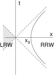
Figure 3: The world line of an accelerated observer. LRW and RRW denote the left- and right-Rindler wedges, respectively. They are the spacelike separated regions with respect to the origin. The accelerated observer intersects the $x$-axis at $x_{0}$.

The field operator $\hat{\phi}(\vec{x},t)$ can be expanded either as the mode sum

$$\hat{\phi}(\vec{x},t)=\sum_{i}\left[u_{i}(\vec{x},t)\,\hat{a}_{M}(u_{i})+{u_{i}(\vec{x},t)}^{\ast}\hat{a}_{M}^{\dagger}(u_{i})\right]\;,$$ (91)

where $\{u_{i}\}$ is an orthonormal basis of positive-frequency (with respect to the timelike Killing field $\partial/\partial t$) solutions of the (Klein-Gordon) field equation for $\phi$ on Minkowski spacetime and $\hat{a}_{M}^{\dagger}(u_{i})$ and $\hat{a}_{M}(u_{i})$ denote the corresponding creation and annihilation operators, or as the mode sum (H.c. is the Hermitian conjugate)

$$\hat{\phi}(\vec{x},t)=\sum_{i}\left[w_{Ri}(\vec{x},t)\,\hat{a}_{R}(w_{Ri})+\mbox{H.c.}\right]\;,$$ (92)

in the right Rindler wedge $\{x>|t|\}$ of Minkowski spacetime (where the accelerating qubit’s worldline is contained), where $\{w_{Ri}\}$ are an orthonormal basis of solutions on the right Rindler wedge which are positive-frequency with respect to the timelike boost Killing field $\hat{a}(x\partial_{t}+t\partial_{x})$ there (which is normalized to have unit length along our qubit’s worldline) and $\hat{a}_{R}^{\dagger}(w_{Ri})$ and $\hat{a}_{R}(w_{Ri})$ denote the corresponding creation and annihilation operators.

There is a similar mode sum for $\hat{\phi}(\vec{x},t)$ on the left Rindler wedge (see UnruhWald ; wald94 for details). The operators $\hat{b}^{\dagger}$ and $\hat{b}$ in Eq. (90) denote the raising and lowering operators in the internal (two-dimensional) Hilbert space of the qubit:

$$\hat{b}|0\rangle=0\;, \hat{b}|1\rangle=|0\rangle\;,$$ (93)

$$\hat{b}^{\dagger}|0\rangle=|1\rangle\;, \hat{b}^{\dagger}|1\rangle=0\;.$$ (94)

Accordingly, the internal Hamiltonian of the qubit is simply

$$H_{0}=\Omega\,\hat{b}^{\dagger}\hat{b}\;,$$ (95)

where $\Omega$ is the energy difference between the ground and excited states.

As first discovered by Unruh Unruh , when the (bosonic) Fock space for the quantum theory of the field $\phi$ is built from the Rindler mode expansion Eq. (92) instead of the Minkowski-mode expansion Eq. (91), the Minkowski vacuum state $|0\rangle_{M}$ can be written in the form

$$|0\rangle_{M}=\prod_{i}\left(C_{i}\sum_{n_{i}}e^{-\pi n_{i}\omega_{i}/a}|n_{i},R\rangle\otimes|n_{i},L\rangle\right)\;.$$ (96)

Here the product is over all Rindler modes of the form $w_{Ri}$ (and the corresponding left-wedge modes $w_{Li}$) with (positive) frequencies $\omega_{i}$, and the inner sum is over all non-negative integers $n_{i}$ with $|n_{i},R\rangle$ and $|n_{i},L\rangle$ denoting the state with $n_{i}$ particles in the mode $w_{Ri}$ and $w_{Li}$ respectively. The normalization constants $C_{i}$ are given by

$$C_{i}\equiv\sqrt{1-e^{-2\pi\omega_{i}/a}}\;.$$ (97)

When the left-Rindler components of the vacuum state $|0\rangle_{M}$ of Eq. (96) are traced-out, the reduced density matrix for Minkowski vacuum as seen by uniformly accelerating observers in the right Rindler wedge is given by

$$\rho_{R}=\prod_{i}\left({C_{i}}^{2}\sum_{n_{i}}e^{-2\pi n_{i}\omega_{i}/a}|n_{i},R\rangle\otimes\langle n_{i},R|\right)\;$$ (98)

which is exactly a thermal state at the Unruh temperature

$$k_{B}T=\frac{a}{2\pi}\;.$$ (99)

V.2 Evolution of the qubit

We are interested in calculating the final state of the qubit when initially, before the acceleration commences, it is in the state

$$|\psi\rangle=\frac{|0\rangle+|1\rangle}{\sqrt{2}}\;.$$ (100)

Let us first assume that initially the qubit is in the ground state $|0\rangle$, and the field is in the Fock state $|n\rangle$ having $n$ particles in the mode corresponding to a one-particle Hilbert space element (positive-frequency solution) $\chi(\vec{x},t)$. So the combined initial state of the field and the qubit is

$$|\mbox{in}\rangle=|n\rangle\otimes|0\rangle\;.$$ (101)

The evolution of this input state under the interaction Hamiltonian Eq. (90) is computed in first order perturbation theory (in the coupling constant $\epsilon$) in UnruhWald , between Eqs. (3.4) and (3.26) there. To state their result, let us introduce the smooth function of compact support

$$f(\vec{x},t)\equiv\epsilon(t)\,e^{i\Omega t}\psi^{\ast}(\vec{x})$$ (102)

and the retarded minus advanced solution of the Klein-Gordon equation with source $f$: ${\cal E}f\equiv Rf-Af$, where $\square(Rf)=\square(Af)=f$. Denote the positive and negative frequency parts of ${\cal E}f$ by $\Gamma_{+}$ and $\Gamma_{-}$, respectively, as in UnruhWald . We have the basic relation

$$\hat{\phi}(f) \equiv \int\hat{\phi}(\vec{x},t)\,f(\vec{x},t)\,\sqrt{-g}\,d^{4}x$$ (103)

$$= \hat{a}(\Gamma^{\ast}_{-})-\hat{a}^{\dagger}(\Gamma_{+})\;$$

expressing the field operator smeared with the test function $f$ in terms of the creation and annihilation operators acting on Fock space. Then, at the end of the acceleration (when $t\gg\Delta$), the final state of the field and the qubit system evolving under the interaction Hamiltonian Eq. (90) is, according to first-order perturbation theory,

$$|\mbox{out}\rangle=|n\rangle\otimes|0\rangle-i\hat{a}(\Gamma^{\ast}_{-})|n\rangle\otimes|1\rangle\;.$$ (104)

Here

$$\hat{a}(\Gamma^{\ast}_{-})|n\rangle = \sqrt{n}(\Gamma^{\ast}_{-},\chi)|n-1\rangle$$ (105)

$$= \sqrt{n}\int\!\!f(\vec{x},t)\chi(\vec{x},t)\sqrt{-g}\,d^{4}x|n-1\rangle\;,$$

where $(,)$ denotes the inner product on the 1-particle Hilbert space of positive-frequency solutions. Assume now that the initial state is

$$|\mbox{in}\rangle=|n\rangle\otimes|1\rangle\;$$ (106)

instead of Eq. (101). The evolution of this input state can be computed in exactly the same way as in UnruhWald , with only slight modifications of their Eqs. (3.18) to (3.25). It follows that at the end of the acceleration (when $t\gg\Delta$), the final state evolving from Eq. (106) according to first-order perturbation theory is

$$|\mbox{out}\rangle=|n\rangle\otimes|1\rangle+i\hat{a}^{\dagger}(\Gamma_{+})|n\rangle\otimes|0\rangle\;,$$ (107)

where

$$\hat{a}^{\dagger}(\Gamma_{+})|n\rangle=\sqrt{n+1}\,\nu\,|\hat{\Gamma}_{+}\otimes_{S}(n\cdot\chi)\rangle\;,$$

$$\nu\equiv\sqrt{(\Gamma_{+},\Gamma_{+})}\;,\;\;\;\;\;\;\hat{\Gamma}_{+}\equiv\Gamma_{+}/\nu\;.$$ (108)

Here $|\hat{\Gamma}_{+}\otimes_{S}(n\cdot\chi)\rangle$ denotes the Fock state that corresponds to the symmetrized product of the $n+1$ normalized positive-frequency solutions (one-particle states): $\hat{\Gamma}_{+}\cdot\chi\cdot\chi\cdots\chi$. Putting together Eqs. (104) and (107), when the initial state of the field and the qubit system is the coherent superposition

$$|\mbox{in}\rangle=|n\rangle\otimes(|0\rangle+|1\rangle)/\sqrt{2}\;,$$ (109)

the outgoing state at the end of the acceleration/interaction episode is

$$|\mbox{out}\rangle = |n\rangle\otimes(|0\rangle+|1\rangle)/\sqrt{2}$$ (110)

$$-i\sqrt{n}(\Gamma^{\ast}_{-},\chi)|n-1\rangle\otimes|1|\rangle/\sqrt{2}$$

$$+i\nu\,\sqrt{n+1}\;|\,\hat{\Gamma}_{+}\otimes_{S}(n\cdot\chi)\,\rangle\otimes|0\rangle/\sqrt{2}\;.$$

The physical interpretation of Eq. (110) is simple: the first term is the zeroth-order unperturbed initial state, the second term corresponds to the absorption of a single quantum of $\phi$-radiation by the qubit, and the third term corresponds to the stimulated emission of a single quantum at the transition frequency $\Omega$. When the initial state of the field is a more general Fock state containing $n_{1}$ particles in mode $\chi_{1}$, $n_{2}$ particles in mode $\chi_{2}$, and so on:

$$|\mbox{in}\rangle=|n_{1},n_{2},\cdots,n_{q}\rangle\otimes(|0\rangle+|1\rangle)/\sqrt{2}\;,$$ (111)

it is not difficult to calculate the appropriate generalization of Eq. (110) for the outgoing state; the result is:

$$|\mbox{out}\rangle=|n_{1},n_{2},\cdots,n_{q}\rangle\otimes(|0\rangle+|1\rangle)/\sqrt{2}$$ (112)

$$- \frac{i}{\sqrt{2}}\sum_{k=1}^{q}\sqrt{n_{k}}(\Gamma^{\ast}_{-},\chi_{k})|n_{1},\cdots n_{k}-1,\cdots,n_{q}\rangle\otimes|1\rangle$$

$$+ \frac{i\nu}{\sqrt{2}}\sqrt{1+\sum_{k=1}^{q}n_{k}}\;|\,\hat{\Gamma}_{+}\!\!\otimes_{S}\!(n_{1}\cdot\chi_{1})\cdots(n_{q}\cdot\chi_{q})\,\rangle\otimes|0\rangle\;.$$

We now have all the machinery we need to compute the evolution of the internal state of an accelerating qubit which is initially in the state Eq. (100). Notice that at no point in the above formalism, Eqs. (101) to (112), we made any reference to the particular construction of the Fock space for the field $\phi$. In particular, the formalism is valid for the Rindler construction based on the mode sum Eq. (92), which is the natural construction of the quantum field theory of $\phi$ from the viewpoint of an observer accelerating with the qubit along the same worldline. According to such an observer, the Minkowski vacuum state in the right Rindler wedge is given by the thermal density matrix Eq. (98). The initial state of the combined field and qubit system at the start of the acceleration is

$$\rho_{\rm in} = \rho_{R}\otimes|\psi\rangle\langle\psi|$$ (113)

$$= \frac{1}{2}\rho_{R}\otimes(|0\rangle+|1\rangle)\otimes(\langle 0|+\langle 1|)\;.$$ (114)

We will now make the formal simplification that the thermal state Eq. (98) contains only one Rindler mode $w_{Ri}=\chi_{\Omega}$, where $\chi_{\Omega}$ is a mode whose frequency $\omega$ equals the transition frequency $\Omega$. This simplification is justified because the overlap factor $({\Gamma^{\ast}}_{-},\chi)$ in the absorption (second) term in Eq. (110) is negligible unless $\chi$ happens to be a mode at a frequency $\omega\approx\Omega$ [see Eq. (105)]. While the spontaneous emission terms into states with other modes are not similarly negligible, they have a trivial form whose contribution is qualitatively the same with or without the simplification. With this assumption, the product over modes in Eq. (98) disappears, and the thermal state of Rindler particles bathing our qubit can be written in the form

$$\rho_{R}={C}^{2}\sum_{n}e^{-2\pi n\Omega/a}|n,R\rangle\otimes\langle n,R|\;,$$ (115)

where

$$C\equiv\sqrt{1-e^{-2\pi\Omega/a}}\;.$$ (116)

The input state of the field and the qubit system, Eq. (113), now takes the simpler form

$$\rho_{\rm in} = \frac{{C}^{2}}{2}\sum_{n}e^{-2\pi n\Omega/a}\left[|n,R\rangle\otimes(|0\rangle+|1\rangle)\right]$$ (117)

$$\quad\otimes\left[\langle n,R|\otimes(\langle 0|+\langle 1|)\right]\;.$$

Each of the components in the sum in Eq. (116) undergoes an evolution as in Eq. (112), ending up at the end of the acceleration in the final state:

$$|n,R\rangle\otimes\frac{|0\rangle+|1\rangle}{\sqrt{2}}\longrightarrow\frac{1}{\sqrt{2Q_{n}}}\Big{[}\;|n,R\rangle(|0\rangle+|1\rangle)$$ (118)

$$- i\sqrt{n}(\Gamma^{\ast}_{-},\chi_{\Omega})|n-1,R\rangle|1\rangle$$

$$+ i\nu\,\sqrt{n+1}\;|\,\hat{\Gamma}_{+}\otimes_{S}(n\cdot\chi_{\Omega})\,,R\rangle\otimes|0\rangle\,\Big{]}\;,$$ (119)

where we used

$$Q_{n}\equiv 1+\frac{n}{2}|(\Gamma^{\ast}_{-},\chi_{\Omega})|^{2}+(n+1)\frac{\nu^{2}}{2}\;.$$ (120)

We have corrected the normalization error affecting Eqs. (104) through (112) which is symptomatic of any approximation based on first-order perturbation theory.

The crucial quantity measuring the strength of the interaction is the overlap $\mu\equiv(\Gamma^{\ast}_{-},\chi_{\Omega})$, which, according to Eqs. (102) and (105), can be calculated as

$$\mu \approx \frac{\epsilon\Delta}{\sqrt{2\Omega}}\int\psi^{\ast}(\vec{x})e^{i\vec{k}_{0}\cdot\vec{x}}\,d^{3}x$$ (121)

$$\approx \frac{\epsilon\Delta}{\sqrt{2\Omega}}\,e^{i\zeta}\,e^{-\frac{1}{2}\kappa^{2}\Omega^{2}}\;,$$

where $\vec{k}_{0}$ denotes the wave vector corresponding to the Rindler mode $\chi_{\Omega}$ (thus $|\vec{k}_{0}|\approx\Omega$, at least for small accelerations $a$), $\kappa$ is a length scale setting the spatial range of the interaction (thus $\psi(\vec{x})$ falls off like a Gaussian distribution with variance $\kappa^{2}$), and $\zeta$ is a phase encoding directional information about $\vec{k}_{0}$ which is irrelevant to our considerations. Similarly to Eq. (121), the quantity $\nu$ [Eq. (V.2)] can be computed as

$$\nu\approx\frac{\epsilon\,\Delta}{2\left(\sqrt{\pi}\kappa^{3}\right)^{1/2}}\;.$$ (122)

Figure 4: The purity ${\rm Tr}(\rho_{q,\rm out}^{2})$ as a function of the acceleration of the qubit. The acceleration is plotted in units of $\Omega$ (i.e. the horizontal axis depicts the dimensionless quantity $a/\Omega$).When there is no acceleration the qubit remains pure (purity$=1$), and for increasing acceleration the qubit approaches the maximally mixed state (purity$=0.5$).

Getting back to the evolution of the input state Eq. (113), combining Eq. (118) with Eq. (117) gives

$$\rho_{\rm out} = \frac{{C}^{2}}{2}\frac{\sum_{n}e^{-2\pi n\Omega/a}}{Q_{n}^{-1}}\Big{[}\;|n,R\rangle\otimes(|0\rangle+|1\rangle)$$ (123)

$$-i\mu\sqrt{n}\,|n-1,R\rangle\otimes|1\rangle$$

$$+i\nu\,\sqrt{n+1}\;|\,\hat{\Gamma}_{+}\otimes_{S}(n\cdot\chi_{\Omega})\,,R\rangle\otimes|0\rangle\;\Big{]}$$

$$\otimes\Big{[}\;\langle n,R|\otimes(\langle 0|+\langle 1|)$$

$$+i\mu^{\ast}\sqrt{n}\,\langle n-1,R|\otimes\langle 1|$$

$$-i\nu\,\sqrt{n+1}\;\langle\,\hat{\Gamma}_{+}\otimes_{S}(n\cdot\chi_{\Omega})\,,R\,|\otimes\langle 0|\;\Big{]}\;.$$

All we need to do now to evaluate the final state of the qubit is to trace over the field degrees of freedom:

$$\rho_{q,\rm out}=\mbox{Tr}_{\phi}\left(\rho_{\rm out}\right)\;.$$ (124)

It is straightforward to calculate this partial trace of Eq. (123) over the Fock space; the result is

$$\rho_{q,\rm out} = \frac{{C}^{2}}{2}\sum_{n}\frac{e^{-2\pi n\Omega/a}}{Q_{n}}\left[(|0\rangle+|1\rangle)(\langle 0|+\langle 1|)\right.$$ (126)

$$\left.+|\mu|^{2}\,n\,|1\rangle\langle 1|+\nu^{2}\,(n+1)\,|0\rangle\langle 0|\right]\;,$$

where [cf. Eq. (118)]

$$Q_{n}=1+n\frac{|\mu|^{2}}{2}+(n+1)\frac{\nu^{2}}{2}\;.$$ (127)

Introducing the sums

$$S_{0} \equiv (1-e^{-2\pi\Omega/a})\sum_{n}\frac{e^{-2\pi n\Omega/a}}{Q_{n}}\;,$$ (128a)

$$S_{a} \equiv (1-e^{-2\pi\Omega/a})|\mu|^{2}\sum_{n}\frac{n\,e^{-2\pi n\Omega/a}}{Q_{n}}\;,$$ (128b)

$$S_{e} \equiv (1-e^{-2\pi\Omega/a})\nu^{2}\sum_{n}\frac{(n+1)\,e^{-2\pi n\Omega/a}}{Q_{n}}\;,$$ (128c)

which satisfy $S_{0}+S_{a}/2+S_{e}/2=1$, Eq. (126) can be written in the more compact form

$$\rho_{q,\rm out}=\frac{1}{2}\left(\begin{array}[]{cc}S_{0}+S_{e}&S_{0}\\ S_{0}&S_{0}+S_{a}\end{array}\right)\;\;.$$ (129)

The purity ${\rm Tr}(\rho_{q,\rm out}^{2})$ can now be expressed as a function of the acceleration; a numerical plot is shown in Fig. 4.

VI Conclusions

In conclusion, we have studied the effect of quantum fluctuations in the spacetime metric on the evolution of a qubit. We considered three general-relativistic paradigms: flat fluctuations in a two-dimensional Minkowski space, mass fluctuations in the Schwarzschild metric for a qubit in a circular orbit, and the interaction of a qubit with coherent and squeezed gravitational waves. Finally, we analyzed the decoherence of an accelerating qubit interacting with the thermal bath of Unruh particles in Minkowski spacetime.

We found that in addition to the expected decoherence of the qubit, flat fluctuations induce a phase drift proportional to the square of the magnitude of the fluctuations. Similarly, mass fluctuations in a black hole induce a phase shift in addition to the decoherence. Gravitational radiation has a peculiar interaction with the qubit, involving periodic episodes of decoherence followed by restoration of coherence for a sinusoidal wave. These periodic episodes disappear when we consider wave packets which, in both the coherent and squeezed states induce a small phase drift proportional to the strength of the field as well as the expected decay of off-diagonal density-matrix elements. The thermal Unruh radiation induces decoherence with a characteristic dependence on the magnitude of the acceleration.

References

• (1) S. Dimopoulos and G. Landsberg, Phys. Rev. Lett. 87, 161602 (2001); S. B. Giddings and S. Thomas, hep-th/0106219.
• (2) T. Jacobson, S. Liberati, and D. Mattingly, hep-ph/0209264.
• (3) U. Yurtsever, Holographic entropy bound and local quantum field theory, Phys. Rev. Lett. (in press).
• (4) M. Czachor, Phys. Rev. A 55, 72 (1997).
• (5) A. Peres, P.F. Scudo, and D.R. Terno, Phys. Rev. Lett. 88, 230402 (2002).
• (6) P.A. Alsing and G.J. Milburn, Quant. Inf. Comp. 2, 487 (2002).
• (7) R.M. Gingrich and C. Adami, Phys. Rev. Lett. 89, 270402 (2002).
• (8) A.J. Bergou, R.M. Gingrich, and C. Adami, quant-ph/0302095.
• (9) P.M. Alsing and G.J. Milburn, quant-ph/0302179.
• (10) H. Lee, P. Kok, and J.P. Dowling, J. Mod. Opt. 49, 2325 (2002).
• (11) S.D. Bartlett, T. Rudolph, R.W. Spekkens, Phys. Rev. Lett., in press, quant-ph/0302111.
• (12) W.G. Unruh and R.M. Wald, Phys. Rev. D 29, 1047 (1984).
• (13) R.M. Wald, Quantum Field Theory in Curved Spacetime and Black Hole Thermodynamics, University of Chicago Press, Chicago (1994).
• (14) W.G. Unruh, Phys. Rev. D 14, 870 (1976).
• (15) U. Yurtsever, Phys. Rev. D 37, 2803 (1988).
• (16) I. Lovas, Heavy Ion Phys. 9, 217 (1999).
• (17) R.M. Wald, General Relativity, University of Chicago Press, Chicago (1984).
• (18) L.P. Grishchuk and Y.V. Sidorov, Phys. Rev. D 42, 3413 (1990).
• (19) E. Zauderer, Partial Differential Equations of Applied Mathematics, Wiley-Interscience (1989).