Schrödinger’s cat and the clock:
Lessons for quantum gravity

Abstract

I review basic principles of the quantum mechanical measurement process in view of their implications for a quantum theory of general relativity. It turns out that a clock as an external classical device associated with the observer plays an essential role. This leads me to postulate a “principle of the integrity of the observer”. It essentially requires the observer to be part of a classical domain connected throughout the measurement process. Mathematically this naturally leads to a formulation of quantum mechanics as a kind of topological quantum field theory. Significantly, quantities with a direct interpretation in terms of a measurement process are associated only with amplitudes for connected boundaries of compact regions of space-time. I discuss some implications of my proposal such as in-out duality for states, delocalization of the “collapse of the wave function” and locality of the description. Differences to existing approaches to quantum gravity are also highlighted.

1 Introduction

In spite of many decades of research a quantum mechanical theory of general relativity still seems out of reach. The opinions as to why this is so are divided, ranging from blaming purely technical difficulties to claiming a fundamental incompatibility between quantum mechanics and general relativity. Although the latter point of view might seem extreme, the persistent failure of reconciling the two frameworks justifies at least a review of fundamental principles. I wish to contribute to such a review by reexamining the measurement process in the context of a quantum description of space-time.

Conventionally, the problem of quantum mechanical measurement is treated as something that can be considered in the context of a classical (and even non-special-relativistic) space-time. This is what the formalism of quantum mechanics is based on. It is then assumed that a quantization of space and time is merely a second step which can be performed within the formalism thus set up.

In contrast to this point of view I emphasize here the desired quantum nature of space and time in the formalization of the measurement process itself. My guiding principle in doing so does not consist of introducing any new postulates or of proposing an alternative to quantum mechanics. Rather, it consists of “taking serious” basic principles of quantum mechanics while not necessarily endorsing every aspect of its standard formalism. Indeed, it is precisely the application of principles of quantum mechanics itself to space-time which prompts me to argue for a modification (or rather generalization) of the standard formalism.

2 Schrödinger’s cat revisited

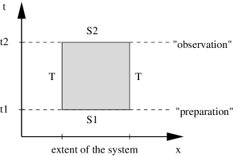
Figure 1: The space-time diagram of the measurement process. Only one spatial dimension is shown. The world-line of the system between preparation at time $t_{1}$ and observation at time $t_{2}$ is the shaded area.

As an illustration of the prototypical quantum mechanical measurement process I recall the thought experiment with Schrödinger’s cat [1]. Assume I take a box into which I put a living cat and a radioactive isotope connected to a mechanism that will kill the cat if a decay is detected. I close the lid (that is, I isolate the system from its environment) and wait for a certain time $t$. Then I open the lid to see whether the cat is dead or still alive. I find (repeating the experiment many times) that the cat will still be alive with a certain probability $p(t)$, but I cannot predict the outcome of any single experiment. Quantum mechanics forbids me to assume that the cat is either definitely dead or definitely alive while I do not look into the box. In other words, it disallows me to assume a definite classical evolution to take place inside the closed box. Indeed, as decades of experimental evidence in quantum mechanics have shown, such an assumption would lead to contradictions. Nevertheless, quantum mechanics allows me to exactly calculate the probability $p(t)$.

Generally, the measurement process involves a quantum domain and a classical domain. The system on which the measurement is performed (here the interior of the box) is part of the quantum domain while the observer is part of the classical domain (here the surroundings). In the quantum domain no definite classical evolution takes place and it does not make sense there to ascribe classical states to the system.

The conventional mathematical description of the experiment is as follows (see Figure 1 for a space-time diagram). Associated with the system is a Hilbert space $\mathcal{H}$ of states. At the time $t_{1}$ I prepare the system in a state $\psi\in\mathcal{H}$ (I set up isotope, machine and cat). Then I isolate the system (I close the lid). I let the system evolve for a time $\Delta t$, which is described by a unitary operator $U(\Delta t)$ acting on $\mathcal{H}$. At time $t_{2}$ I perform the observation (I open the lid). That is, I can ask whether the system is in a state $\eta\in\mathcal{H}^{*}$ (e.g. if the cat is still alive). The probability $p$ that this is the case is the modulus square of the corresponding transition amplitude:

$$p(\Delta t)=|\langle\eta|U(\Delta t)|\psi\rangle|^{2}.$$

3 The cat and the clock

So far I have implicitly assumed that space and time provide a fixed classical background structure. Now I want to treat them as quantum mechanical entities as well. If I take serious the principle that I can know nothing classical about the interior of the box while I do not look inside then this must also extend to space and time. In particular, I must not assume any definite (classical) passage of time inside the box. Outside the box on the other hand time remains a classical entity as part of the classical domain of my observations.

To examine the implications of this I need to pay more attention to how the notion of time enters into my measurement process. I thus refine the description of the experiment as follows: Next to the box I put a clock. After closing the lid I continuously watch the clock until I find that the time $\Delta t$ has elapsed. Then I proceed to open the lid and look inside the box. Of course, the outcome of the experiment is as before, I observe the same probability $p$ of the cat still being alive as a function of $\Delta t$.

But how can this be? How does the system “know” about the time $\Delta t$ elapsed on my clock when I cannot assume any definite evolution of time inside the closed box?

The sensible answer seems to be that the system does stay in contact with its environment while the lid is closed. More precisely, it stays in contact with the space-time as classically experienced by me as the observer. The information about the space-time structure surrounding the box is a boundary condition to the experiment. It encodes in particular the elapsed time $\Delta t$ on the clock. This boundary condition must be regarded an integral part of the quantum mechanical measurement process.

Of course, the focus on the time variable just serves to emphasize my point. What is relevant are both, time and space. Indeed, it is important that I do not move around the box after closing the lid. For example, I do not allow the box to be taken away to (say) Alpha Centauri C and brought back so that the time dilatation would alter the function $p(\Delta t)$ and thus the outcome of my measurements. Even with space-time behaving completely classically the inclusion of this boundary condition into the measurement process can be useful. With a quantum mechanical space-time it becomes inevitable.

4 Integrity of the observer

On the conceptual level I can view the above argument also as stating something about the observer. Let me call this the principle of the integrity of the observer. This means that the whole measurement process (including preparation and observation proper) pertains to one connected classical domain in which the observer describes reality. In the above thought experiment this connectedness is manifest in the clock and in me as the observer watching the clock while the box is closed.

A measurement distributed over several disconnected classical domains does not make sense. An observer in one of them would have to relate to other ones either through classical channels of communication or via interaction through the quantum domain. In the first case the classical domains would be connected into just one classical domain. In the second case the other classical domains effectively become part of the quantum domain. Applied to the prototypical experiment described above this means that it does not make sense for the observer to consider preparation and observation as disconnected interactions between classical and quantum domains. To the contrary, to relate the two it is essential that the observer has a classical existence in between (with a classical time duration $\Delta t$).

5 Criticism: The clock in the box

Before proceeding I would like to meet one possible criticism of my interpretation of the thought experiment with Schrödinger’s cat. I have argued that the elapsed time $\Delta t$ on my clock next to the box is something about which the system inside the box cannot “know” anything in the conventional interpretation of the experiment. But what if I put the clock inside the box? Upon opening the box I could correlate this internal time $\Delta t_{i}$ to the probability of finding the cat dead or alive. I would obtain the same probability distribution as above. It seems that this way of looking at the experiment does not require any kind of contact between system and outside world while the lid of the box is closed.

But I have a problem now. After closing the lid, when shall I open it again to look for the cat (and the clock)? As the clock is inside the box I cannot look at it while I wait. (Indeed this is essential for it to be part of the quantum domain.) Shall I think of the time of opening the box as somehow “random”? But how? Perhaps I should view this as somebody else preparing the experiment for me and sending me a closed box. This I open and determine both $\Delta t_{i}$ and the state of the cat. But as there is no such thing as an a priori random distribution of the $\Delta t_{i}$ this might not tell me anything. For example, in the repetitions that I arrange it could be that the $\Delta t_{i}$ is always astronomically large and the cat always dead.

The point is that the modification fundamentally changes the experiment. It does not provide me with the same information as the original experiment. The fact that I can predetermine the elapsed time $\Delta t$ is an essential part of the original experiment. The modified experiment thus corresponds to a different measurement process. Apart from that, it is not even clear whether this modified measurement process can be made sense of without introducing some classical connection between preparation (even if this is done by “somebody else”) and observation through the back door. For example, what distribution of times $\Delta t_{i}$ am I supposed to observe opening many boxes?

A different strategy would be to put a clock outside the box as well. But then, how do I explain that the external and internal clocks show the same elapsed time (up to quantum fluctuations)? This leads me back to my original argument.

6 Encoding the boundary condition

Let me propose a formalization of the consequences of the thought experiment. To this end I shall assume that I can strictly identify classical and quantum domain with corresponding regions of space-time. In the present experiment the quantum domain is thus the world 4-volume of the box in the time interval $[t_{1},t_{2}]$ (the shaded area in Figure 1). The classical domain is everything outside. (This assumption will turn out to be stronger than required.)

Now, how exactly is the ambient classical space-time a boundary condition to the experiment? According to quantum mechanics the interaction between observer and system (preparation and observation) should take place at the interface between the classical and quantum domains. Thus, the relevant spatio-temporal information should reside in the metric space-time field on the three-dimensional boundary that separates the two. This three-dimensional connected boundary $B$ consists of three parts (see Figure 1): the space-like boundary $S_{1}$ consisting of the inside of the box at the time $t_{1}$ of preparation, the time-like boundary $T$ of the spatial boundary of the box while waiting for the time $\Delta t$ to elapse and again the space-like boundary $S_{2}$ of the inside of the box at the time $t_{2}$ of observation.

To what extent a metric on a connected surface such as $B$ determines or over-determines a solution of the Einstein equations inside is a difficult initial value problem. Due to the similarity with the “thick sandwich” problem [2] I shall assume that the intrinsic metric is sufficient. However, the exact validity of such an assumption is probably not a crucial ingredient for a quantum theory of general relativity.

7 Quantum general relativity as a TQFT

To calculate a transition amplitude I need thus three pieces of information: The initial state $\psi$ on $S_{1}$, the final state $\eta$ on $S_{2}$ and the intrinsic metric $g$ on the whole of $B=S_{1}\cup T\cup S_{2}$. This suggests a mathematical description as follows: Associated with $B$ is a state space $\mathcal{H}_{B}$ and I can think of $(\psi,\eta,g)$ as determining an element in this space. (In a truly quantum description of space and time I should think of $g$ really as a quantum state “peaked” at a classical metric rather than a classical metric itself.) The amplitude for such a state is given by a map $\rho:\mathcal{H}_{B}\to\mathbb{C}$. The associated probability (density) $p$ is as usual the modulus square of the amplitude, i.e.

$$p=|\rho(\psi,\eta,g)|^{2}.$$

To recover the conventional mathematical description of the experiment the state space can be split into a tensor product corresponding to the boundary components $\mathcal{H}_{B}=\mathcal{H}_{S_{1}}\otimes\mathcal{H}_{T}\otimes\mathcal{H}_{S_{2}}$. Correspondingly, I label the metric living on the different components by $g_{1},g_{T},g_{2}$. Then I should recover $\mathcal{H}=(\mathcal{H}_{S_{1}}|g_{1})$, i.e. the state space $\mathcal{H}$ is the space of states in $\mathcal{H}_{S_{1}}$ which are partly fixed to $g_{1}$ (namely in their metric information), correspondingly $\mathcal{H}^{*}=(\mathcal{H}_{S_{2}}|g_{2})$. I call $\mathcal{H}$ and $\mathcal{H}^{*}$ reduced state spaces. The amplitude is then equal to

$$\rho(\psi,\eta,g)=\langle\eta_{g_{2}}|U(g_{T})|\psi_{g_{1}}\rangle.$$

The indices on the states indicate that they live in the reduced state spaces with fixed metric and the argument of $U$ that it depends (apart from the state spaces $\mathcal{H}$ and $\mathcal{H}^{*}$) on the metric $g_{T}$. Note that in particular, $g_{T}$ contains the information about the time duration $\Delta t$.

The mathematical structure of the formalization I have given above is essentially that of a topological quantum field theory (TQFT) [3]. Let me briefly recall what this means in the present context. The basic setting is that of topological (or rather differentiable) manifolds in dimension four. Associated to any 3-boundary $B$ of a 4-manifold $M$ is a vector space $\mathcal{H}_{B}$ of states. Associated to $M$ is a map $\rho_{M}^{B,\emptyset}:\mathcal{H}_{B}\to\mathbb{C}$. If $B$ is the union of components $B=B_{1}\cup B_{2}$ the space $\mathcal{H}_{B}$ is the tensor product of spaces associated with the components $\mathcal{H}_{B}=\mathcal{H}_{B_{1}}\otimes\mathcal{H}_{B_{2}}$. Besides considering boundaries as “in” I can also regard them as “out” whereby the corresponding space is replaced with its dual and appears in the codomain of $\rho$ instead of its domain. For example, regarding $B_{1}$ as “in” and $B_{2}$ as “out” I would have $\rho_{M}^{B_{1},B_{2}}:\mathcal{H}_{B_{1}}\to\mathcal{H}_{B_{2}}^{*}$.

Figure 2: Gluing two manifolds along a common boundary corresponds to composition in TQFT.

A crucial property of a TQFT is the composition property: The gluing of two 4-manifolds at a common boundary corresponds to the composition of the respective maps. More precisely, consider a 4-manifold $M_{1}$ with boundaries $B_{1}$ and $B_{2}$ and a 4-manifold $M_{2}$ with boundaries $B_{3}$ and $B_{4}$. Then I have maps $\rho_{M_{1}}^{B_{1},B_{2}}:\mathcal{H}_{B_{1}}\to\mathcal{H}_{B_{2}}^{*}$ and $\rho_{M_{2}}^{B_{3},B_{4}}:\mathcal{H}_{B_{3}}\to\mathcal{H}_{B_{4}}^{*}$. Assume that $B_{2}$ and $B_{3}$ are mirror images so that $M_{1}$ and $M_{2}$ can be glued together (see Figure 2). This also implies $\mathcal{H}_{B_{2}}^{*}=\mathcal{H}_{B_{3}}$. The composition property then states for $\rho_{M_{1}\cup M_{2}}^{B_{1},B_{4}}:\mathcal{H}_{B_{1}}\to\mathcal{H}_{B_{4}}^{*}$ associated with the union $M_{1}\cup M_{2}$ that

$$\rho_{M_{1}\cup M_{2}}^{B_{1},B_{4}}=\rho_{M_{2}}^{B_{3},B_{4}}\circ\rho_{M_{1}}^{B_{1},B_{2}}.$$

If I consider the special case of boundaries that are equal-time-slices in Euclidean or Minkowski space I recover the usual formulation of quantum mechanics. The composition property corresponds then to the summation over a complete set of intermediate states.

However, my point is that I allow more general boundaries (and here I go beyond the use that is usually made of TQFT in physical contexts). In particular, boundaries might have time-like components and I may glue along such boundaries. Rather than a composition of time-evolutions this would be a composition in space. Physically, this might for example correspond to the formation of a composite system out of separate systems. Since this is really a “quantum” composition in the same sense as the composition of time-evolutions is, the consistency of this operation is ensured.

8 In-out duality

An implication of allowing rather arbitrary boundaries is that the distinction between “in” and “out” states of quantum mechanics becomes arbitrary, in turn blurring the distinction between preparation and observation proper in the measurement. Even the “in” and “out” notions of TQFT become inadequate. More precisely, they become purely technical notions that can essentially be turned around at will (by dualization, see above). The physical notions of “in” (as preparation) or “out” (as observation) become necessarily disentangled from this technical one. For example, in the above thought experiment certain data associated with the boundary component $S_{2}$ was considered “out” (the reduced state $\eta$) while certain other data on the same $S_{2}$ (the metric or quantum state of space-time $g_{2}$) was considered “in”.

So how is this separation into physical “in” and “out” encoded? The answer is that there is no need for it. This is not really a surprise. Indeed, quantum field theory has been teaching us this lesson for a long time. It is manifest in a remarkable feature of the LSZ reduction [4]. Consider the time ordered correlation function (in momentum space) of $n$ fields,

$$\langle 0|T\phi(p_{1})\cdots\phi(p_{n})|0\rangle.$$

Its modulus square is a probability density – and in several ways. Given incoming particles with momenta $p_{1},\dots,p_{k}$ it is essentially the probability density for observing outgoing particles with momenta $p_{k+1},\dots,p_{n}$. How many particles I regard as incoming (i.e. which value I take for $k$) is arbitrary. For each choice the right answer is given by the very same quantity. How I split up the “state” into prepared part (corresponding to $\psi$ above) and observed part ($\eta$ above) is arbitrary. Note though that exchanging “in” and “out” states requires to exchange positive with negative energy. But this fits the associated orientation reversal in the time direction of the TQFT description.

In the same sense the function $\rho$ is to be regarded as giving an amplitude for a state $\psi$. Whether a part of this state is to be considered as prepared or as observed does not alter the associated probability density. It is rather to be viewed as an ingredient of the experimental circumstances. This appears to be a rather strong postulate in general but I hope to have made it plausible through well established physics.

The removal of the a priori distinction between preparation and observation proper might also be seen as having implications for the interpretation of quantum mechanics. In the conventional picture I can think that I prepare the system in the state $\psi$ at time $t_{1}$, after which it evolves deterministically to the state $U(\Delta t)\psi$. Then I perform the observation at time $t_{2}$ and the wave function “collapses”. This description of course no longer makes sense in the proposed formulation. There the boundary is connected and it seems rather far-fetched to associate a “collapse” with any particular piece of this boundary (especially if it has a quite arbitrary shape). Instead one could still talk about a “collapse” but this would have to be associated with the boundary as a whole. In particular, it is no longer localized in time and thus cannot have the usual connotation of the “instantaneous disruption” of a deterministic evolution.

9 Connectedness of the boundary

Above I have argued how the thought experiment naturally leads to a TQFT description of quantum mechanics. Significantly, the principle of the integrity of the observer implies the connectedness of the boundary at the interface between classical and quantum domain. That is, a TQFT amplitude can only have a direct interpretation in terms of a quantum mechanical measurement process (that involves a quantum treatment of space-time) if it is associated with a connected 3-boundary.

One might object that ordinary quantum mechanics gets along very well with disconnected boundaries. But this I would argue, is due rather to simplifications (especially due to the fixed space-time background) than fundamental reasons. A typical system of interest has a finite extent. Outside this extent nothing relevant happens that requires really a quantum mechanical treatment. Comparing this to Figure 1, nothing interesting happens at the boundary $T$ and it might be neglected and conveniently pushed to infinity. The situation becomes different however, when space-time is no longer regarded as a fixed background but treated quantum mechanically as well. As I have argued, the boundary $T$ then plays an essential role.

Note that this argument also remains valid if the system is infinitely extended. The crucial point is that the observer remains excluded so that there is a boundary between him and the system. Pushing this further we might even “invert” the picture of Figure 1 and consider the observer’s world line as surrounded by a boundary outside of which “the quantum mechanics happens”. I will not pursue this point of view here though.

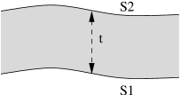
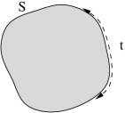
(a)		(b)

Figure 3: (a) The more traditional approach to quantum gravity employs space-like boundaries $S_{1}$ and $S_{2}$. (b) The advocated approach employs connected boundaries $S$ of compact regions of space-time.

The connectedness of the boundary is rather significant for the interpretation of theories of quantum gravity and quantum cosmology. Let me compare this to the more traditional point of view that is often adopted in approaches to quantum gravity (e.g. in the Wheeler–DeWitt approach [5, 6], in Euclidean quantum gravity [7] and also in loop quantum gravity [8]). Consider two space-like boundaries (say Cauchy surfaces) $S_{1}$ and $S_{2}$ which are closed and extend “to infinity” in the universe (see Figure 3.a). One then considers transition amplitudes between quantum states of the metric on $S_{1}$ and on $S_{2}$. The question how a time duration $\Delta t$ (along some path) between an event on $S_{1}$ and an event on $S_{2}$ is to be encoded is then answered as follows: Given a solution of Einstein’s equations consider the two non-intersecting spatial hypersurfaces $S_{1}$ and $S_{2}$. Then, generically, it is conjectured that this solution can be reconstructed (up to diffeomorphism) given the intrinsic metrics on $S_{1}$ and $S_{2}$. (This is the “thick sandwich” problem [2].) This implies that such intrinsic metrics contain the information about the time difference in the above sense. At least for quasi-classical states in a suitable sense it should be appropriate to talk about time durations $\Delta t$ (with some uncertainty) between “initial” and “final” state.

Nevertheless, this approach has the disadvantage that it cannot be directly related to a measurement process of the type considered above. What I called the principle of the integrity of the observer is violated. To remedy this I would presumably have to fix some spatial region (where I as the observer live) and its world-line to be classical. But this would essentially amount to introducing extra boundary components that connect $S_{1}$ and $S_{2}$, thus introducing a connected boundary through the back door. In the proposed approach the relevant boundary $S$ is connected from the outset (see Figure 3.b). There is no need to refer to temporal distances “between” boundaries. Temporal (or spatial) distances related to a measurement process can be evaluated on paths on the boundary using the intrinsic metric only.

10 Locality

Apart from an analysis of the measurement process there are other reasons to look for a TQFT type description of quantum gravity using compact connected boundaries. An important reason is locality.

Compact connected boundaries allow for an adaption of the mathematical description to the size of the system considered. There is no need a priori to include things (even empty space) at infinity. Of course, going to infinity might not change the mathematical description much or might even simplify it (e.g. asymptotic states in quantum field theory). However, while this is certainly true in quantum mechanics and quantum field theory on Minkowski space, it is very unlikely to be true in a non-perturbative theory of quantum gravity.

Let me also mention that the program of Euclidean quantum gravity uses compact manifolds and connected boundaries. However, there the motivation is a mathematical one rather than a physical one. Indeed the interpretation of corresponding quantities in that program markedly differs from the interpretation that emerges in the present context. For example, there one can define a “wave function of the universe” [9]. Here the interpretation of essentially the same mathematical quantity would be as giving rise to a functional on states that yields the amplitude for a local measurement process on the boundary of a finite region of space-time. This will be elaborated elsewhere.

Talking about states or wave functions “of the universe” is often motivated by “realist” interpretations of quantum mechanics, such as the many-worlds interpretation (as clearly expressed in [5] for example). What I mean by this (without being precise) is that one assigns a physical reality to the wave function independent of any measurement process. One might argue that such a point of view has no support from our experimental evidence on quantum mechanics. I do not wish to take sides in this debate here but emphasize that the local point of view put forward here requires no particular interpretation of quantum mechanics to be adopted a priori.

11 Topological versus topological

There is a folklore saying that classical general relativity is not a topological theory and hence its quantization cannot be a topological quantum field theory. However, this is in my view due to a misuse of the word “topological”. In the first instance it refers to the classical theory having no local degrees of freedom, in the second to the fact that the background structures of the quantum theory are topological manifolds and their cobordisms (although “differentiable” would be more appropriate here). The second does not imply the first. Indeed, consider the classical limit. Then states on boundaries as in Figure 3 which are “peaked” at a classical metric, determine up to diffeomorphisms essentially a unique classical solution of general relativity “inside”. There is no reason to think that a quantum theory cannot incorporate this, for example as the dominant contribution to a path integral. Indeed, this is for example a vital ingredient of the Euclidean quantum gravity program.

One should not be misled by the fact that many interesting TQFTs that have been constructed can be viewed as quantizations of topological theories (e.g. [10]). This seems rather related to the fact that the vector spaces associated with boundaries there are finite dimensional (which would not be expected for quantum gravity).

12 Conclusions and Outlook

In the non-relativistic context of the founding days of quantum mechanics the picture of initial state, evolution and final state was quite appropriate. I have argued that it becomes inadequate when including space and time in the quantum mechanical realm itself. Of course, I am not the first to express such a sentiment. However, I have based my argument on the very principles of the quantum mechanical measurement process itself. Furthermore, I have proposed a way out, namely by adopting a TQFT type description for a quantum theory of general relativity. Links between TQFT and quantum general relativity have been suggested before (e.g. [11]), even to the extent of proposing a TQFT formulation [12]. The physical interpretations, however, were rather different from the one put forward here. This is also the case for other previous physical applications of TQFT which generally maintain space-like boundaries.

This proposal has a number of implications. Among them are a somewhat radical departure from the “static” Hilbert space picture of quantum mechanics. Related to that is a necessary duality between “in” and “out” states, or preparation and observation. In particular, states are physically meaningful even if associated with boundaries that have time-like components. For the interpretation of quantum mechanics conclusions might be drawn, in particular the necessary “delocalization” in time of the “collapse of the wave function”. It also implies a shift in the interpretation of quantities in present approaches to quantum gravity (e.g. the “wave function of the universe”).

At the moment what I have presented is a proposal only, and many crucial details are missing. It stands and falls with the feasibility of formulating quantum theory in a “general boundary” way. Although designed for a quantum theory of general relativity this can be adapted also to ordinary quantum mechanics and quantum field theory. Then, the background structure is not that of topological (or differentiable) manifolds but metric manifolds, i.e. one would have a “metric quantum field theory”. At first sight the definition of “particle” seems to be a major obstacle. Surprisingly, it appears that such a formulation is nevertheless possible (at least for standard cases) for both quantum mechanics and perturbative quantum field theory, and in a rather uniform way. This will be demonstrated in forthcoming publications [13].

Note that the present proposal also goes some way to suggest how to modify present approaches to quantum gravity, with a view towards obtaining physically meaningful amplitudes. This applies notably to loop quantum gravity [8] and spin foam models [14, 15]. A first step would be the introduction there of boundaries with both space- and time-like components. The interpretation of amplitudes should then become clearer once the quantum mechanics and quantum field theory situations have been worked out.

Acknowledgements

I would like to thank Carlo Rovelli for stimulating discussions, Thomas Schücker for a critical reading of the manuscript and Domenico Giulini for providing me with a reference. This work was supported through a Marie Curie Fellowship of the European Union.

References

- [1] E. Schrödinger, Die gegenwärtige Situation in der Quantenmechanik, Naturwiss. 23 (1935), 807–812, 823–828, 845–849.
- [2] J. A. Wheeler, Geometrodynamics and the Issue of the Final State, Relativity, Groups and Topology (C. DeWitt and B. DeWitt, eds.), Gordon and Breach, New York, 1964, pp. 315–520.
- [3] M. Atiyah, Topological quantum field theories, Inst. Hautes Études Sci. Publ. Math. (1989), no. 68, 175–186.
- [4] H. Lehmann, K. Symanzik, and W. Zimmermann, Zur Formulierung quantisierter Feldtheorien, Nuovo Cimento 1 (1955), 205–225.
- [5] B. S. DeWitt, Quantum Theory of Gravity. I. The Canonical Theory, Phys. Rev. 160 (1967), 1113–1148.
- [6] J. A. Wheeler, Superspace and the Nature of Quantum Geometrodynamics, Batelle Rencontres (C. M. DeWitt and J. A. Wheeler, eds.), W. A. Benjamin, New York, 1968, pp. 242–307.
- [7] S. W. Hawking, The path-integral approach to quantum gravity, General Relativity: An Einstein Centenary (S. W. Hawking and W. Israel, eds.), Cambridge University Press, Cambridge, 1979.
- [8] C. Rovelli, Loop Quantum Gravity, Living Rev. Rel. 1 (1998), 1.
- [9] J. B. Hartle and S. W. Hawking, Wave function of the Universe, Phys. Rev. D 28 (1983), 2960–2975.
- [10] E. Witten, Quantum Field Theory and the Jones Polynomial, Commun. Math. Phys. 121 (1989), 351–399.
- [11] L. Crane, Topological field theory as the key to quantum gravity, Knots and quantum gravity (Riverside, CA, 1993), Oxford Lecture Ser. Math. Appl., no. 1, Oxford Univ. Press, New York, 1994, pp. 121–132.
- [12] J. W. Barrett, Quantum gravity as topological quantum field theory, J. Math. Phys. 36 (1995), 6161–6179.
- [13] R. Oeckl, A "general boundary" formulation for quantum mechanics and quantum gravity, to appear in Phys. Lett. B, Preprint hep-th/0306025.
- [14] D. Oriti, Spacetime geometry from algebra: spin foam models for non-perturbative quantum gravity, Rep. Progr. Phys. 64 (2001), 1703–1757.
- [15] A. Perez, Spin foam models for quantum gravity, Class. Quantum Grav. 20 (2003), R 43.