Finding apparent horizons and other two-surfaces of constant expansion

Abstract

Apparent horizons are structures of spacelike hypersurfaces that can be determined locally in time. Closed surfaces of constant expansion (CE surfaces) are a generalisation of apparent horizons. I present an efficient method for locating CE surfaces. This method uses an explicit representation of the surface, allowing for arbitrary resolutions and, in principle, shapes. The CE surface equation is then solved as a nonlinear elliptic equation.

It is reasonable to assume that CE surfaces foliate a spacelike hypersurface outside of some interior region, thus defining an invariant (but still slicing-dependent) radial coordinate. This can be used to determine gauge modes and to compare time evolutions with different gauge conditions. CE surfaces also provide an efficient way to find new apparent horizons as they appear e.g. in binary black hole simulations.

1 Introduction

Apparent horizons serve several purposes during the numerical evolution of general relativistic spacetimes. In vacuum, spacetime has no other prominent features that can be determined locally in time, such as e.g. the shock waves found in hydrodynamics. Event horizons are global structures, and it is not possible to find them during a time evolution, as the future of the spacetime is not yet known. Yet an apparent horizon indicates, under reasonable assumptions, that there is an event horizon present at or outside the apparent horizon. Furthermore, apparent horizons are also under certain circumstances isolated horizons, making it then possible to calculate their mass and spin [1, 2, 3].

Locating apparent horizons is also necessary when one wants to apply excision boundary conditions in a numerical time evolution, where the apparent horizon is used to determine the location and shape of the excised regions. It is therefore important to have a fast and robust apparent horizon finder that is closely integrated with the evolution code.

Apparent horizons can be generalised to closed two-surfaces of constant expansion (CE surfaces). Empirically, CE surfaces lead to a foliation of a spacelike hypersurface outside of some interior region. Often, the gauge in which numerical solutions to Einstein’s equations are obtained is itself the result of time evolution equations, so that the gauge condition is not known explicitly. CE surfaces can be used to define a radial coordinate that is independent of the spatial gauge choice. This allows to determine gauge modes and compare different gauge conditions.

This article is structured as follows. Section 2 introduces the notation and gives the defining equations for apparent horizons and surfaces of constant expansion. Section 3 explains the discretisation of the surfaces and the numerical methods used to solve the equations. Section 4 shows tests with analytic solutions and compares the finder’s accuracy and speed to existing implementations of apparent horizon finders. Finally, section 5 presents hypersurface foliations and apparent horizon pre-tracking as applications for CE surfaces, and section 6 summarises the results.

2 Definitions

A marginally outer-trapped surface is a two-surface within a spacelike hypersurface with zero expansion and spherical topology. An apparent horizon is the outermost such surface. The condition that it be an outermost such surface is difficult to verify in practice, and I will follow the current usage to disregard this condition.

Therefore, at each point of an apparent horizon, the condition $H=0$ has to hold, where

$$H:=\nabla_{i}s^{i}+K_{ij}(s^{i}s^{j}-\gamma^{ij})$$ (1)

is the so-called apparent horizon function (see e.g. [4, 5]). Here $s^{i}$ is the (spacelike) outward normal to the horizon, and $\gamma_{ij}$ and $K_{ij}$ are the three-metric and extrinsic curvature of the spacelike hypersurface.

A generalisation of apparent horizons, which have zero expansion, are surfaces that have instead a certain constant expansion $\lambda$. These CE surfaces are defined through a condition $H_{\lambda}=0$, where

$$H_{\lambda}:=H-\lambda$$ (2)

is the CE surface function. Apparent horizons are CE surfaces with $\lambda=0$. In asymptotically spacelike foliations of asymptotically flat spacetimes, coordinate spheres with $r\to\infty$ are CE surfaces with $\lambda=2/r$. Figure 1 (a) shows as examples the behaviour of $\lambda$ vs. $r$ for coordinate spheres in some spherically symmetric spacetimes.

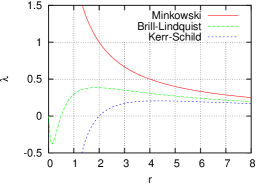
(a)        (b)

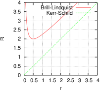
Figure 1: (a) Expansion $\lambda$ vs. coordinate radius $r$ for the Minkowski, a Brill–Lindquist ($\mu=1$), and a Kerr–Schild ($M=1$) metric. All curves tend to $\lambda=2/r$ for $r\to\infty$. Apparent horizons are located where $\lambda=0$. (b) Areal radius $R$ vs. coordinate radius $r$ for a Brill–Lindquist ($\mu=1$) and a Kerr–Schild ($M=1$) metric. Note that for Kerr–Schild coordinates $R=r$. The apparent horizons are here located where $R=2$.

In the case of a vanishing extrinsic curvature, CE surfaces are also constant mean curvature surfaces (CMC surfaces). These lead under certain assumptions, such as a positive energy density, to a foliation of the spacelike hypersurface outside a small interior region [6]. It is not unreasonable to assume the CE surfaces will also lead to a foliation under similar conditions, although this has not yet been proven.

It is clear from figure 1 (a) that the expansion $\lambda$ is not monotonic and therefore cannot be used to define a radial coordinate. However, such an invariant radial coordinate would be most useful for numerical simulations, e.g. to compare results obtained with different gauge conditions, or to have some insight into the coordinate distortions caused by a gauge condition.

If the CE surfaces have monotonically increasing areas, then it is natural to consider the areal radius

$$R=\sqrt{A/4\pi}$$ (3)

of a surface, where $A$ is the area of the surface as measured using the three-metric in the spacelike hypersurface. This areal radius is twice the irreducible mass for an apparent horizon. (It is also equal to the radial coordinate $r$ when the radial gauge $\gamma_{\theta\theta}=r$ is used in spherical symmetry.) Figure 1 (b) shows as examples the behaviour of the areal radius of coordinate spheres for some spherically symmetric spacetimes.

In order for $R$ to be a useful coordinate in practice, it is necessary that one be able to find a CE surface with a specific areal radius $R$. It is not always possible to locate such a surface by considering CE surfaces with varying values of $\lambda$, because varying $\lambda$ is ill-defined where the gradient of $\lambda$ vanishes (see again figure 1 (a)). Instead, I define the areal-radius-corrected CE surface function

$$H_{r}:=H-\bar{H}+(R-r)/r$$ (4)

which is zero if and only if the trial surface is a CE surface with the areal radius $r$. Here $\bar{H}$ is the average of the expansion of the surface, i.e. $\bar{H}=\int d\Omega\,H(\Omega)/4\pi$. $R$ is the surface’s areal radius as defined by equation (3) above. As all correction terms are scalars, i.e. constant on the surface, $H_{r}$ can only be constant for a CE surface. The term $H-\bar{H}$ vanishes for a CE surface, hence $H_{r}=0$ only if $R=r$, which is intended.

3 Numerical issues

The above definitions are only useful in numerical relativity if there is an efficient method to find CE surfaces with a specific expansions $\lambda$ or specific areal radii $R$. This section describes such a method, explaining how the surfaces are represented and discretised and how equations (1), (2), and (4) are then solved.

Thornburg [4] gives a rather complete overview of current methods of locating apparent horizons, many of which could also be applicable for finding surfaces of constant expansion after suitable adaptation. Baumgarte and Shapiro [7] review many issues related to numerical relativity, including locating apparent horizons.

3.1 Representation of the surface

Surfaces with spherical topology can be represented explicitly by a function $h(\theta,\phi)$ that specifies (this is an arbitrary choice) the radius $r$ as a function of the spherical coordinates $\theta$ and $\phi$. This choice restricts the possible surfaces to those of star-shaped regions about some origin, but this restriction does not cause problems in practice; other choices would be equally possible. The surface consists of those points $(r,\theta,\phi)$ of the spacelike hypersurface that satisfy the condition $r=h(\theta,\phi)$.

The surface can also be defined implicitly through an expression $F(x^{i})=0$, with the level set function $F$ defined e.g. as

$$F(r,\theta,\phi):=r-h(\theta,\phi)\quad\textrm{.}$$ (5)

This representation leads to the equation

$$s_{i}=\frac{\nabla_{i}F}{|\nabla F|}$$ (6)

for the outward normal, where $|\nabla F|:=\left(\gamma^{jk}\,\nabla_{j}F\,\nabla_{k}F\right)^{\frac{1}{2}}$. The function $F$ and the spacelike normal $s^{i}$ can be calculated using either spherical coordinates $(r,\theta,\phi)$, or transformed to use Cartesian coordinates $(x,y,z)$. Such coordinate distinctions are rather important for the numerical implementation of an algorithm, so that I will not pass over them below.

3.2 Coordinates on the surface

The above choice of spherical coordinates to parameterise the surface introduces a preferred coordinate system into the otherwise coordinate independent equations (1), (2), and (4). Another preferred coordinate system typically comes from the grid used in the time evolution code for the whole spacetime. Often, $\gamma_{ij}$ and $K_{ij}$ are given in Cartesian components on a Cartesian grid. This raises the question as to which coordinate system to use in the numerical implementation of the horizon finder. The coordinate choice will of course not influence the physical results, but it can make the implementation more complicated if it requires interpolation, or considerably less accurate if it leads to coordinate singularities. It can also make the results more or less difficult to interpret, as tensor quantities are numerically always expressed through their coordinate components. Tensors in different coordinate systems cannot easily be compared, even if they are given at the same grid points. In short, the choice of a coordinate system is numerically an important issue.

I choose to represent the quantities on the surface using their fully three-dimensional Cartesian tensor components, even when they only live on the two-dimensional surface. This has the advantage that the tensors $\gamma_{ij}$ and $K_{ij}$ do not have to have their components transformed, although they do need to be interpolated to the location of the surface.

The overall advantage of using Cartesian tensor components is that coordinate singularities at the poles do not influence the representation of such quantities. While the singularities will still influence the calculation of derivatives intrinsic to the surface, the representation of the results will not have coordinate singularities any more. Vector and tensor components in spherical coordinates would either tend to zero or diverge at the poles.

I use the indices $i$, $j$, $k$ for Cartesian components ($i,j,k\in[x,y,z]$), $u$, $v$, $w$ for spherical components in 3D ($u,v,w\in[r,\theta,\phi]$), and $a$, $b$, $c$ for spherical components on the surface ($a,b,c\in[\theta,\phi]$). This convention distinguishes which quantities are defined on what manifold, and also makes coordinate transformations explicit.

3.3 Discretisation of the surface

The discretisation scheme of the three-dimensional quantities, i.e. those living on the whole spacelike hypersurface, does not play a role when locating a CE surface. There only has to be a way to interpolate these quantities onto the surface. These quantities are often discretised on a Cartesian grid. It is also possible to use spherical coordinates, or to use mesh refinement, without influencing the way in which the apparent horizon function $H$ is evaluated.

I choose to discretise the two-dimensional quantities, i.e. those quantities living on the surface, by using a polar $\theta$-$\phi$-grid with constant grid spacings $d\theta$ and $d\phi$. A constant grid spacing works well when the surface has a shape that is not too far from a sphere. Experiments show that distorted (peanut-shaped) horizons still work fine, but usually require a higher resolution.

Polar coordinates create coordinate singularities at $\theta=0$ and $\theta=\pi$, which I avoid by having the grid points staggered with respect to the poles. The boundary condition in the $\phi$-direction is periodic: $f(\theta,\phi)=f(\theta,\phi+2\pi)$ for any function $f$ living on the surface. The boundary condition in the $\theta$-direction, i.e. across the poles, is a bit more involved. It is $f(\theta,\phi)=P\cdot f(-\theta,\phi+\pi)$ for arbitrary tensor components $f$, where the parity $P=(-1)^{k}$ depends on the rank $k$ of the tensor of which $f$ is a component. Figure 2 demonstrates the polar boundary condition, especially how the shift by $\pi$ in $\phi$-direction comes about. (See also [8].)

(a)        (b)

Figure 2: (a) North pole of the grid on the sphere, in a polar projection. This shows the grid lines as they lie on the sphere. (b) North pole of the grid on the sphere, as seen from the grid. The black and white dots have multiple images on the coordinate grid, separated by $\pi$ in the $\phi$-direction.

This grid allows numerical partial derivatives to be taken only in the $\theta$- and $\phi$-directions. Equations (1) and (6) also need $r$-derivatives, and these cannot be taken numerically. However, the $r$-derivatives of the coordinate transformation operators are known analytically, and one can see from the definition of $F$ that $\partial_{r}F=1$ by construction. Finally, the partial derivatives of the three-metric, which are given in Cartesian coordinates, are calculated before the metric is interpolated onto the surface.

My choice of evaluating the apparent horizon function directly on the grid that forms the surface while retaining the Cartesian coordinate system for the tensor components seems to be an uncommon one. It is also possible to evaluate the apparent horizon function not on the surface itself, but instead in the three-dimensional spacetime on those grid points that are close to the surface [4, 9, 10]. This method requires interpolating in both directions between the surface and the spacelike hypersurface. It also has the disadvantage that the domain of the equation, i.e. the set of active grid points, changes with the surface, leading to further complications.

While I represent the shape of the surface using an explicit grid, one different way that is commonly used is to expand the surface shape in spherical harmonics [11, 12, 13, 14, 5]. An expansion in spherical harmonics does not have coordinate singularities. Furthermore, one has direct insight into and control over the high spatial frequency components. A multipole representation is by definition restricted to star-shaped regions, while an explicit representation is generic; however, this disadvantage is not important in practice. More problematic is that integrations over the surface are rather expensive, as they scale with $O(\ell_{\mathrm{max}}^{4})$, were $\ell_{\mathrm{max}}$ is the number of multipole moments used. With an explicit grid, these integrations scale with $O(n)$, where $n$ is the number of grid points, and where one should choose $n=O(\ell_{\mathrm{max}}^{2})$ for a fair comparison. On the other hand, multipole expansions converge faster than finite difference discretisations. (I present run time comparisons in section 4.2 below.)

Other possible ways to represent the surface without coordinate singularities could use several overlapping grid patches [15], finite elements, or hierarchical bases [16].

3.4 Evaluating the CE surface functions

I use the algorithm described below to evaluate the apparent horizon function $H$. From that, the CE surface functions $H_{\lambda}$ and $H_{r}$ can be calculated.

Although the quantities $F$, $s^{i}$, and $H$ are defined everywhere in space, they only need to be evaluated on the trial surface, i.e. on the surface determined by $h$. They still need to be defined in a neighbourhood of the surface, so that their $r$-derivatives can be taken. Their continuation off the surface is chosen arbitrarily, and is here implicitly determined by the above choice of spherical coordinates. Thus the finder calculates quantities on the two-dimensional surface only, although the quantities live in three dimensions.

It would be a bad idea to calculate the derivatives of $s^{i}$ numerically, as $s^{i}$ is itself already calculated as a derivative. Taking a derivative of a derivative leads to an effective stencil that is twice as large and that contains elements with a weight of zero. These zero weights lead to an even–odd decoupling of the grid points, which in turn leads to large solution errors. Instead, one uses the chain rule and calculates $\nabla_{i}s^{i}$ directly from second derivatives of $F$. This makes it necessary to calculate $\nabla_{i}\nabla_{j}F$ and $\nabla_{i}s^{i}$ numerically along with $\nabla_{i}F$ and $s^{i}$.

Algorithm

1. Assume that the three-metric $\gamma_{ij}(x^{k})$ and the extrinsic curvature $K_{ij}(x^{k})$ are given as fixed background quantities in the whole spacelike hypersurface. These quantities do not change while the CE surface is located.

2. Assume that a 2-surface $h(x^{a})$ has been chosen for which the apparent horizon function is to be evaluated. This is e.g. done by an elliptic solver as described below.

3. Calculate the surface grid point locations in Cartesian coordinates as $x^{i}(x^{a})$, using the definition of $h$.

4. Interpolate the three-metric, the extrinsic curvature, and the partial derivatives of the three-metric onto the surface. These quantities can be viewed conceptually as representing $\gamma_{ij}(x^{u})$ and $K_{ij}(x^{u})$, but are stored as $\gamma_{ij}(x^{a})$, $K_{ij}(x^{a})$, and $\partial_{k}\gamma_{ij}(x^{a})$. (The partial derivatives are needed later.) Note that these tensors now live on the surface, but still have their components as Cartesian components.

5. Define the implicit surface location $F(x^{u})=F(r,\theta,\phi)=r-h(\theta,\phi)$. This quantity is not stored explicitly.

6. Calculate an outward-directed covector $\nabla_{v}F(x^{u})$ that is orthogonal to the surface. By definition, $\partial_{r}F=1$, and $\partial_{a}F=-\partial_{a}h$. This is stored as $\partial_{v}F(x^{a})$ and $\partial_{v}\partial_{w}F(x^{a})$. (The second derivatives are needed later). The calculation needs the values $\partial_{b}h(x^{a})$ and $\partial_{b}\partial_{c}h(x^{a})$, which are calculated on the surface.

7. Define the transformation operator $T_{i}^{u}$ that transforms from spherical to Cartesian covariant coordinate components on the surface. This operator is given by $T_{i}^{u}$ = $\partial x^{u}/\partial x^{i}$, where the $x^{i}(x^{u})$ are given by the usual relations

   $$x=r\sin(\theta)\cos(\phi)\quad\quad y=r\sin(\theta)\sin(\phi)\quad\quad z=r\cos(\theta)\quad\textrm{.}$$

   Evaluate this operator and its derivatives at $r=h$, and store them as $T_{i}^{u}(x^{a})$ and $\partial_{j}T_{i}^{u}(x^{a})$.

8. Transform the components of the outward-directed covector into spherical coordinates: $\nabla_{i}F(x^{u})=T_{i}^{v}\,\nabla_{v}F(x^{u})$. Store $\nabla_{i}F(x^{a})$ and $\nabla_{i}\nabla_{j}F(x^{a})$. The calculation of the second derivatives needs the derivatives of the transformation operator $T$, and also needs the partial derivatives of the three-metric for the connection coefficients.

9. Normalise the outward-directed covector $\nabla_{i}F(x^{u})$ and raise its index to $s^{i}(x^{u})=\gamma^{ij}\nabla_{j}F(x^{u})$. Calculate its derivative $\nabla_{i}s^{i}(x^{u})$. This needs the second derivatives of $F$. Store $s^{i}(x^{a})$ and $\nabla_{i}s^{i}(x^{a})$.

10. Calculate the apparent horizon function $H=\nabla_{i}s^{i}+K_{ij}(s^{i}s^{j}-\gamma^{ij})$. Store it as $H(x^{a})$.

For the above calculation I use a second-order accurate interpolator, and second-order centred differences to approximate the partial derivatives. Altogether, the apparent horizon function $H$ thus depends on the background spacetime as given by $\gamma_{ij}$ and $K_{ij}$, and on the surface location $h$.

3.5 Solving the CE surface equations

I follow the idea presented in [17, 18, 4, 19, 8, 9] to interpret the apparent horizon and CE surface equations as elliptic equations on the surface. Commonly used other methods for apparent horizon finding are mean curvature flow [20] or level flow methods [10], or minimisation procedures [14]. The advantages of flow methods for horizon finding are that they are in general more robust in finding a horizon, and that they are in practice able to find an outermost, i.e. true apparent horizon, given a large enough sphere as initial data. Their disadvantage is that they lead to parabolic or degenerate elliptic equations that are very expensive to solve. Minimisation procedures can also lead to a more stable formulation than elliptic formulations, but are usually much slower. I will restrict myself here to the solution of elliptic equations. As described below, I have also implemented a simple Jacobi solver that is conceptually identical to a flow method.

It is possible to change the nature of equations (1), (2), and (4) by extending them to the three-dimensional spacelike hypersurface. This is done by changing from the unknown function $h(\theta,\phi)$ to a level set $h_{q}(\theta,\phi)$, where $q$ is a level set parameter [20]. The advantage of such an extension is that multiple CE surfaces can be found at the same time. The disadvantage is that such an extension has a higher numerical cost because of the additional dimension. However, such a method would be ideal to find the whole set of CE surfaces that make up a foliation at once. Unfortunately, one would have to know in advance what region of the hypersurface is not covered by the foliation, and impose a corresponding inner boundary condition.

The conditions $H=0$, $H_{\lambda}=0$, and $H_{r}=0$ are all nonlinear elliptic equations in $h$, as can be seen by substituting the definitions of $s^{i}$ and $F$ into $H$. Strictly speaking, only the equations $|\nabla F|\,H=0$ etc. are elliptic. But this additional factor is often close to unity, and omitting it makes then little difference for nonlinear elliptic solvers.

In order to solve a nonlinear equation, one needs initial data, which are in this case an initial guess for the surface location. These initial data select which CE surface will be found — if there are several present on the spacelike hypersurface — or whether any will be found at all. During a time evolution one can easily use the location from the previous time step as initial data; this works very well in practice and is called tracking. However, finding CE surfaces in an unknown spacetime is more difficult. Depending on how e.g. the initial configuration for a time evolution run is constructed, one does not know where or of what shape the CE surfaces are.

I have implemented this CE surface finding algorithm within the Cactus framework [21], which has gained some popularity in the numerical relativity community. I hope that this will make it easier for other people to use this implementation not only as an external program, but also directly from within their code. Within Cactus, I have examined two different nonlinear elliptic solvers for the CE surface equations, a Newton-like method and a flow-like method.

3.5.1 Newton method

The faster of the two solvers uses a Newton-like method to reduce the nonlinear equation to a linear one, and then a standard solver for the linear problem (GMRES with ILU preconditioning). This is implemented by interfacing to the PETSc library [22, 23]. While this solver is very fast (it usually takes less than a second to converge), it also converges only if one starts sufficiently close to the final location and shape. In particular, it has problems with finding distorted surfaces when starting with a sphere and vice versa.

PETSc needs the Jacobian of the elliptic equation in order to solve the system. I chose to represent the Jacobian explicitly as a sparse matrix. It is then necessary to have a routine that creates the structure of the non-zero elements of this Jacobian. In doing so one has to make sure that the grid point couplings due to the boundary conditions (see figure 2) are treated correctly. PETSc can then calculate the values of the non-zero entries through numeric differentiation, which is usually slow, but is in this case fast enough. Although PETSc also offers matrix-free methods, i.e. solvers that only use implicit representations of the matrix, I did not use them, because they can lead to convergence problems that are difficult to investigate.

This solver does not always work when solving for CE surfaces with a specified areal radius $R$. I assume that this is because I only use an approximation to the Jacobian in this case. The term $\bar{H}$ in equation (4) leads to a fully populated Jacobian, whereas I ignore the $\bar{H}$ term when I calculate it.

One large advantage of PETSc is that it can easily be reconfigured through options at run time to use a variety of different solvers and preconditioners. It can also explicitly calculate all eigenvalues of a system (if the system is small), which is very helpful for understanding convergence properties.

3.5.2 Flow method

The other, more robust solver is a Jacobi solver, which is conceptually identical to a mean curvature flow solver, as e.g. described in [24, 10]. (It should probably rather be called an expansion flow solver, as the flow really is governed by the surface’s expansion and not its mean curvature.) This solver converges very reliably to the desired CE surface if the step size is chosen to be small enough. A Jacobi solver solves in effect a parabolic equation, so that the maximum stable step size scales with the square of the surface resolution. This requires very small step sizes unless the surfaces resolution is very coarse. That means that this solver requires very long run times of the order of minutes, or tens of minutes if one starts far away from the solution.

The maximum stable step size depends on the equation’s eigenvalues, which are unknown because the equation is nonlinear. I have therefore implemented a primitive adaptive step size control mechanism which monitors the norm of the residual. As long as the residual decreases while iterating, the step size is slowly increased (e.g. by 10% per step). If the residual increases, the step size is sharply decreased (e.g. by a factor of 10). I find that it is not necessary to undo steps that increase the residual; on the contrary, such steps usually increase the convergence rate. I assume that such overshooting gives this algorithm some SOR-like properties. This mechanism, which surely could be improved upon, chooses step sizes which usually lead to a stable integration, while it also adapts to the stability criteria that change with the flowing surface.

Of course, even adaptive step size control does not lead to a truly fast algorithm for a parabolic equation. In order to accelerate this solver, I often use a hybrid approach: I start by using the flow solver, but do not wait until it has fully converged. After some time I switch to using PETSc, with the output of the flow solver as the starting point. This combines the robustness of the flow solver in finding unknown shapes with the fast convergence rate of PETSc once an approximate solution is known.

4 Tests

4.1 Tests with analytic solutions

As first test for the convergence properties of this method, I use a single black hole in Kerr–Schild coordinates (see e.g. section 3.3.1 of [25] for a definition). Table 1 contains results from runs with a black hole of mass $M=1$ and spin $a=0$. The table compares the irreducible mass of the horizon with the ADM mass of the whole spacelike hypersurface which I calculate numerically for reference (see e.g. equation (7.6.22) in [26]). I would consider the resolutions $1/4$, $1/8$, and $1/16$ to be coarse, reasonable, and fine, respectively, for a numerical representation of this spacetime.

Table 1: Left: Horizon and ADM masses for a black hole with $M=1$ and $a=0$. $R/2$ is the irreducible mass of the horizon where $A=4\pi R^{2}$ is its area, and $M_{\mathrm{ADM}}$ is the ADM mass of the whole spacelike hypersurface. Both the spacetime and the surface vary in resolution. The last row gives the analytic values. Right: Convergence factors for these results. A value of 4 indicates second order convergence.

• run	$dx$	$d\phi$	$R/2$	$M_{\mathrm{ADM}}$
  a	$1/4$	$2\pi/36$	0.991111	1.00043
  b	$1/8$	$2\pi/72$	0.997693	1.00010
  c	$1/16$	$2\pi/144$	0.999429	1.00002
  	$0$	$0$	1.0	1.0

  runs	$R/2$	$M_{\mathrm{ADM}}$
  a, b, c	3.79	4.43
  a, b	3.85	4.37
  b, c	4.04	4.18

The same table also shows the convergence factors for three-way and two-way convergence tests from the above runs. The convergence factors $f$ are calculated in the usual way via $f=(v_{1}-v_{2})/(v_{2}-v_{3})$ or $f=(v_{1}-v_{a})/(v_{2}-v_{a})$, where $v_{1}$, $v_{2}$, $v_{3}$, and $v_{a}$ represent the coarse, medium, fine grid, and analytic values, respectively. A factor of 4 indicates second-order convergence. The results demonstrate that a spatial resolution of $dx=1/4$ is not sufficient to be in the convergent regime, and also that the numerical ADM masses reported here might not be very accurate.

In another convergence test, shown in table 2, I keep the spatial resolution of the spacelike hypersurface constant at $dx=1/8$, and vary only the resolution of the surface grid. This time the black hole has a mass $M=1$ and a spin $a_{z}=1/2$, again in Kerr–Schild coordinates. The apparent horizon spin $a_{z}$ is estimated via its equatorial circumference as described below. The last line of the table shows the analytic values.

Table 2: Left: Horizon masses, spins, and ADM masses for a black hole with $M=1$ and $a_{z}=1/2$. Only the resolution of the surface varies. The last row gives the analytic values. Right: Convergence factors for these results. A value of 4 indicates second order convergence.

• run	$d\phi$	$R/2$	$a_{z}$	$M$
  A	$2\pi/36$	0.960886	0.496507	0.994655
  B	$2\pi/72$	0.964675	0.498183	0.998537
  C	$2\pi/144$	0.965594	0.498815	0.999511
  D	$2\pi/288$	0.965819	0.498997	0.999754
  	0	0.965926	0.5	1.0

  runs	$R/2$	$a_{z}$	$M$
  A, B, C	4.13	2.65	3.99
  B, C, D	4.08	3.47	4.01

Because it is known in this case that the apparent horizon has a spin that is aligned with the $z$ axis and that the horizon is not distorted, one can use the area and the equatorial circumference to calculate the spin magnitude and the total mass. In the elliptic coordinates that one prefers for Kerr black holes (see e.g. section 3.3 of [25]), a horizon with mass $M$ and spin $a$ is located at the coordinate radius $r$, has the area $A$ and the equatorial circumference $L$, which are given by:

$$r=M+\sqrt{M^{2}-a^{2}}\quad\quad A=4\pi\,(r^{2}+a^{2})\quad\quad L=2\pi\,(r^{2}+a^{2})/r$$ (7)

(I thank Badri Krishnan for pointing out the last equation to me.) These equations can be solved for $a$ and $M$.

The convergence factors for the above test are also shown in table 2. As the spacetime is now fixed, and differs slightly from the analytic solution due to the discretisation errors, I omit the two-way convergence tests here. While the estimate for the total mass $M$ that is calculated this way has a reasonable accuracy, the spin estimate does not converge to second order for these resolutions. This is unfortunate, but not of much consequence, as this method for calculating the spin is not applicable in general anyway.

4.2 Comparison to other apparent horizon finders

I compare the accuracy and speed of the elliptic method described in this article to two other commonly used apparent horizon finding methods, namely the fast flow algorithm presented in [13] and a minimisation procedure described in [14]. Implementations for both are publicly available with the Cactus code [21] and have been described in [5]. Both expand the apparent horizon surface in spherical harmonics. They are part of the Cactus infrastructure, are used in production runs, and have been thoroughly optimised for speed.

As test bed I use a black hole in Kerr–Schild coordinates with $M=1$ and $a_{z}=0.6$, discretised on a Cartesian grid with $dx=1/8$. The horizon is then located at $r=M+\sqrt{M^{2}-a^{2}}=1.8$, which corresponds to the coordinate location $x^{2}+y^{2}+z^{2}=\rho^{2}=r^{2}+a^{2}(1-z^{2}/r^{2})=3.6-z^{2}/9$. In these coordinates, the apparent horizon is thus a slightly oblate ellipsoid; the polar coordinate radius is $\rho_{\mathrm{po}}\approx 1.868$ and the equatorial coordinate radius is $\rho_{\mathrm{eq}}\approx 1.897$. The apparent horizon has octant symmetry (although the spacetime does not), and I enforce it explicitly.

I set up two test cases for these data. In the first case I start with a distorted, oblate surface, and let the finders converge to the horizon. The initial surface has a polar radius of $\rho_{\mathrm{po}}=2$ and an equatorial radius of $\rho_{\mathrm{eq}}=3.5$, or $\ell_{0}\approx 3$ and $\ell_{2}\approx-0.45$ in spherical harmonics (with the normalisations as described in [5]). This is supposed to mimic a situation where not much is known about the spacetime, so that the initial guess is far from the solution. In the second test case I start with a sphere at $\rho=2$, i.e. close in location and shape to the actual horizon. This allows the use of much faster algorithms. This situation is similar to horizon (or CE surface) tracking.

I use the three finders each with two different configurations. For the elliptic method I choose the configurations depending on the test case. For the first test case, I first use the Jacobi solver, and then follow up by calling PETSc, as described in section 3.5.1 above. For the second test case that corresponds to horizon tracking, I use only PETSc. For the fast flow method and the minimisation procedure I use once the default configuration suggested by the authors of the implementation, and once an adapted configuration with more multipole moments and a coarser spatial resolution of the surface.

The numerical resolution of the spacelike hypersurface leads to about $4\pi\rho^{2}\,dx^{2}\approx 2800$ grid points “on” the horizon, i.e. about $350$ on the octant that is represented numerically. For the explicit surface representation in the elliptic method I use $12^{2}=144$ grid points. For the adapted configuration of the fast flow method and the minimisation procedure, I attempt to choose settings for the spherical harmonics that are equivalent to the settings for the explicit surface representation. I decided to limit the expansion to $\ell_{\mathrm{max}}=12$, which leads to $28$ nonvanishing spherical harmonic coefficients due to the octant symmetry. This expansion still has a lower spatial resolution than $12^{2}=144$ explicit grid points, but spherical harmonics have better approximation properties, as can also be seen from the errors in the result. The number $\ell_{\mathrm{max}}=12$ is suggested as “high enough” in the documentation of the code. These adapted settings should also accelerate the fast flow method and the minimisation procedure, leading to a fairer comparison of the run times.

Table 3 lists the exact parameters used for the finders. Table 4.2 compares the physical results, i.e. area, equatorial circumference, mass, and spin as calculated via equations (7). The methods using a decomposition in spherical harmonics apparently slightly depend on the initial data. They also have a higher accuracy. Table 5 lists the run times that the finders took on a Pentium III processor with 1200 MHz, i.e. on reasonable hardware in 2003. The elliptic method with the explicit surface representation is more than an order of magnitude faster at horizon tracking. When the resolution of the fast flow method is reduced down to $\ell_{\mathrm{max}}=4$, then the run time diminishes to $4.10$ seconds, which is still considerably larger than for the explicit representation. Run times are important during a time evolution run, because a horizon finder has to run at every (or every few) time step(s). In order to determine a CE surface foliation, the finder even has to run many times for each hypersurface.

Table 3: Configurations of the horizon finders. $\ell_{\mathrm{max}}$ is the highest term in the spherical harmonic expansion. $n_{\theta}$ and $n_{\phi}$ are the number of grid points on the surface. (The fast flow solver and the minimisation procedure need an explicit surface for surface integrals.)

• minimisation
  	default	adapted
  $\ell_{\mathrm{max}}$	$8$	$12$
  $n_{\theta}$	$100$	$12$
  $n_{\phi}$	$100$	$12$

  fast flow
  	default	adapted
  $\ell_{\mathrm{max}}$	$8$	$12$
  $n_{\theta}$	$100$	$12$
  $n_{\phi}$	$100$	$12$

• elliptic/flow
  $n_{\theta}$	$12\quad$
  $n_{\phi}$	$12\quad$
  flow iterations	$20000\quad$
  flow step size	$10^{-4}$
  error tolerance	$10^{-8}$

  elliptic/PETSc
  $n_{\theta}$	$12\quad$
  $n_{\phi}$	$12\quad$
  error tolerance	$10^{-8}$

Table 4: Results for different configurations and horizon finder algorithms. As expected, the expansion in spherical harmonics leads to a better representation of the surface. Note that the analytic values in the last row are not exact, as they do not take the discretisation of the spacelike hypersurface into account.

• configuration	finder	$A$	$L$	$R/2$	$a_{z}$	$M$
  1 (finding)	minim. (default)	45.146	12.554	0.94770	0.59962	0.99902
  1 (finding)	minim. (adapted)	45.086	12.554	0.94710	0.60279	0.99902
  1 (finding)	elliptic (flow)	44.843	12.513	0.94452	0.59803	0.99574
  2 (tracking)	fast flow (default)	45.224	12.562	0.94852	0.59891	0.99965
  2 (tracking)	fast flow (adapted)	45.131	12.558	0.94755	0.60212	0.99933
  2 (tracking)	elliptic (PETSc)	44.843	12.513	0.94452	0.59803	0.99574
  reference values		45.239	12.566	0.94868	0.6	1.0

  Table 5: Run times for different configurations and horizon finder algorithms. The elliptic method with the explicit surface representation is very fast at horizon tracking.

  • configuration	finder	time [s]
    1 (finding)	minim. (default)	98.94
    1 (finding)	minim. (adapted)	91.45
    1 (finding)	elliptic (flow)	190.43
    2 (tracking)	fast flow (default)	26.97
    2 (tracking)	fast flow (adapted)	10.82
    2 (tracking)	elliptic (PETSc)	0.50

  5 Applications of CE surfaces

  5.1 Comparing different coordinate systems

  Empirically, surfaces of constant expansion seem indeed to foliate spacelike hypersurfaces. Assuming that this is true in general, they can be used to compare spacetime metrics that are given in different coordinate systems. As CE surfaces and thus the foliations depend on the slicing, this requires that equivalent slicings are obtained in some way. That is in general a difficult problem, and I only want to mention two simple ways here. One trivial way is to restrict oneself to considering time-symmetric initial data, where one can compare the results of varying parameters such as black hole configurations or the numerical resolution. Another way is to perform a time evolution, starting with identical initial data and using a maximal slicing condition, comparing results e.g. obtained with different shift conditions or with different numerical parameters.

  In order to demonstrate comparing different metrics, I use in the following an artificial setup with known properties. I compare two metrics of identical stationary Kerr–Schild black hole spacetimes, where a coordinate transformation has been applied to the second metric. I choose the coordinate transformation so that it changes the three-metric only and does not modify the slicing of the spacetime. The different three-metrics lead to different extrinsic curvatures as functions of the three-coordinates.

  I use Kerr–Schild black holes with $M=1$ and $a_{z}=0.6$. The apparent horizon in this spacetime is also an isolated horizon. The transformation is a compression along the $z$ axis by a factor of $0.5$, and a shear in the $x$-$z$ plane by a factor of $0.5$. In this case, the spacetime is deformed by a single, global, linear transformation, so that the spin can still be described by a direction vector.

  I calculate the Killing vector field on this horizon in the way described in [3]. This Killing vector field, shown in figure 3, defines the direction of the spin, putting the “poles” of the spin at $(\theta,\phi)=(0.257\pi,0)$ and $(0.743\pi,\pi)$, which is close to the real values $(\pi/4,0)$ and $(3\pi/4,\pi)$. From the Killing vector field also follow a spin magnitude of $a=0.601$ and a total mass of $M=0.997$, which are also close to the real values.

  

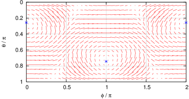
  Figure 3: Killing vector field $\xi^{a}$ on the apparent horizon in the $\theta$-$\phi$ plane. The $z$ axis penetrates this plane at $\theta=0$ and $\theta=\pi$, the positive $x$ axis at $\theta=\pi/2$, $\phi=0$. The two singular points where $\xi^{a}=0$ (marked by the stars) are the black hole’s “poles” defined by the spin.

  Figure 4 shows a cut in the $x$-$z$ plane through the numerically located CE surfaces in the transformed metric, where the direction of the spin is also indicated. It also shows the same cut through the undistorted black hole for comparison. The Killing vector field and the horizon area could be used to define invariant lines of latitude and longitude, providing a complete invariant coordinate system within the spacelike hypersurface. Section VI of [3] discusses a different and slicing-independent method to obtain such a coordinate system.

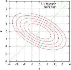
  (a)        (b)

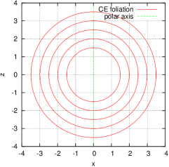
  Figure 4: (a) CE foliation of the transformed Kerr–Schild black hole with $R=\frac{3}{2},\frac{4}{2}\cdots\frac{7}{2}$ (from inner to outer surface). The $R=2$ surface is the apparent horizon. The axis of the black hole is defined by its spin, as shown in figure 3. (b) CE foliation of the undistorted Kerr–Schild black hole for comparison for the same values of $R$. The $R=2$ surface is again the apparent horizon.

  5.2 Detecting coordinate distortions

  Surfaces of constant expansion are useful even when there is no apparent horizon present, where they can be used to detect distorted coordinate systems. Especially when the spacetime is the result of a time evolution, it is difficult to judge how much of an observed distortion is caused by the gauge condition. Surfaces of constant expansion can here serve as anchors, because they are defined independently of the gauge choice that is contained in the three-metric.

  CE surfaces can be considered to be a generalisation of spheres in Euclidean geometry. (In the case of vanishing extrinsic curvature, CE surfaces have constant mean curvature, which is a defining criterion of a sphere.) It is thus justified to define an adapted “undistorted” coordinate system by requiring that CE surfaces be coordinate spheres in it. A related condition, namely that constant mean curvature surfaces be coordinate spheres, has been proposed as a condition for the radial shift vector during time evolution [27]. Invariant lines of latitude and longitude could be obtained by defining them at spatial infinity and propagating them inwards perpendicular to the CE surfaces.

  I consider here an axisymmetric, subcritical Brill wave [28] as example. The three-metric can be written as

  $$ds^{2}=\psi^{4}\left[e^{2q}(d\rho^{2}+dz^{2})+\rho^{2}d\phi^{2}\right]$$ (8)

  with the free function $q(\rho,z)$. I use the Holz source function

  $$q=A\,\rho^{2}\,e^{-r^{2}}$$ (9)

  with the amplitude parameter $A$. $\rho$ is here the cylindrical radial coordinate with $\rho^{2}=x^{2}+y^{2}$. The initial data are chosen to be time-symmetric. Constructing these data involves a numerical solution of the Hamiltonian constraint.

  I choose the amplitude $A=4$ and calculate a CE foliation of these data, shown in figure 5. The CE surfaces near $R=2$ are quite far from coordinate spheres. This distortion is not an intrinsic property of the gravitational wave content; rather, it is only a property of this particular coordinate system. Figure 6 compares the equatorial and polar circumferences of the CE surfaces, showing that these surfaces are prolate, although they have an oblate coordinate shape in the Brill coordinate system. The same shape parameter, albeit for event horizons, is used in [29] to detect quasinormal modes of black holes.

  

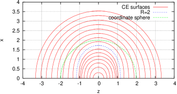
  Figure 5: CE foliation of an axisymmetric Brill wave. Displayed is a cut through the $x$-$z$ plane. (Note the directions of the coordinate axes.) The CE surfaces have areal radii $R=\frac{1}{4}\ldots 4$ in steps of $\frac{1}{4}$; the surface with $R=2$ is emphasised. Note the coordinate distortion of the CE surfaces; a coordinate sphere with $r=2$ is drawn for comparison. There is no apparent horizon present.

  

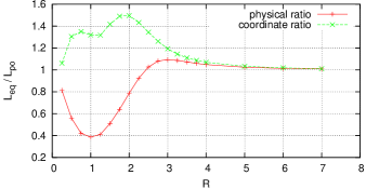
  Figure 6: Ratio between the equatorial and polar physical circumferences for the Brill wave CE surfaces. Values smaller than $1$ indicate a prolate surface, values larger than $1$ an oblate surface. For comparison the ratio of the corresponding coordinate circumferences is also shown.

  5.3 CE surfaces for multiple black holes

  In order to prepare and analyse initial data for binary black hole collision runs, I superpose two Kerr–Schild black holes as proposed in [30], and then solve the constraint equations. This results in spacetimes with either two separate or a single distorted (“merged”) black hole(s). One can freely specify the locations, momenta, masses, and spins of the black holes prior to the superposition. The relation to the properties of the superposed black holes is not known, but it is hoped that the superposition will not change them by much.

  For the superposition, I choose a grid spacing of $dx=1/4$, an outer boundary that has a distance $8$ from the centres of the black holes, and excise a spherical region with radius $1$ around the singularities. I superpose the three-metric and the extrinsic curvature without attenuation. I then solve the constraint equations numerically using the York-Lichnerowicz method with a conformal transverse-traceless decomposition. (This method is described e.g. in section 2.2.1 of [25].) At the outer boundary I use a Dirichlet condition for the vector potential and a Robin condition for the conformal factor. At the excision boundaries I use Dirichlet conditions, keeping the boundary values from the superposition.

  Whether or not a common apparent horizon exists is a hint as to whether the black hole configuration contains two separate or a single merged black hole(s); this fact is not known otherwise. The only way to find out would be to evolve this configuration for a long enough time so that the event horizon could be tracked backwards in time. This is unfortunately not easily possible (if at all) with today’s black hole evolution methods.

  Figure 7 compares common and individual CE surfaces for two superposed Kerr–Schild black holes with $M=1$ and $a=0$ at $z=\pm 2.0$. This configuration is axisymmetric about the $z$ axis and has a reflection symmetry about the $x$-$y$ plane. The system has a common apparent horizon. The individual CE surfaces do not extent far outwards; they cease to exist for values of $R\gtrsim 3$. Similarly, the common CE surfaces do not extend arbitrarily far inwards, ceasing to exist for $R\lesssim 2.7$. It is also clear that there is no smooth transition between the two foliations. However, there is an overlap between the regions in which the different foliations are valid. In both foliations the area increases monotonically outwards, as shown in table 6.

  

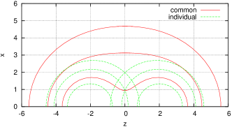
  Figure 7: Common and individual CE surfaces for superposed Kerr–Schild black holes with singularities at $z=\pm 2.0$. (Note the directions of the coordinate axes.) The expansions and areal radii are compared in table 6. The middle common CE surface is the outermost apparent horizon. The middle individual CE surfaces are also apparent horizons.

  Table 6: Expansions and areal radii for the CE surfaces shown in figure 7. The largest individual CE surface shown has a larger expansion (and areal radius) than the smallest shown common CE surface.

  • common
    $\;\;\;\lambda$	$R$
    $+0.1$	$5.053$
    $\;\;\;0.0$	$3.804$
    $-0.25$	$2.713$

    individual
    $\;\;\;\lambda$	$R$
    $+0.1$	$2.952$
    $\;\;\;0.0$	$2.389$
    $-0.5$	$1.494$

  5.4 Apparent horizon pre-tracking

  During a time evolution simulation, new apparent horizons may appear. One does in general not know their location and not even their time of appearance in advance. The new apparent horizon can be formed in a collapse, or it can be the common horizon in a binary black hole coalescence. [10] describes a mechanism in an apparent horizon finder that automatically detects whether a two black hole system has a common horizon, and if not, finds the two separate horizons instead. However, this flow finder is slow, and it is not feasible to apply it at every time step during a time evolution. Except for choosing various trial surfaces as initial guesses and testing whether one of them converges to an apparent horizon, there is no other way to find out whether a new apparent horizon has appeared. This is a slow and cumbersome method.

  Surfaces of constant expansion offer a more efficient approach here. Apparent horizon pre-tracking is an algorithm by which a CE surface with decreasing expansion $\lambda$ is tracked during a binary black hole time evolution before a common apparent horizon has formed. It is much faster to track a surface that is a candidate for an apparent horizon than to examine the spacelike hypersurfaces anew at each time step.

  Pre-tracking works as follows. One starts with a CE surface that “tightly” encloses both singularities. If this surface is sufficiently large, then it will have a positive expansion $\lambda$. This surface is tracked in time. At each time step of the evolution, one iteratively tries to find a surface with as small an expansion as possible. In practice, this minimum possible expansion will vary only slowly with time. Finding a surface with a smaller expansion is very fast, because a surface with a larger expansion is already known and can serve as an initial guess. As soon as a surface with an expansion of zero can been found, a new apparent horizon has been detected.

  This method allows the locating of new apparent horizons as soon as they appear. The current value of $\lambda$ is also an indication as to how close the spacelike hypersurface is to having an apparent horizon near the CE surface.

  As an example I consider a system of two Brill–Lindquist black holes. I do not want to go into the problems associated with the time evolution of a two black hole system, where one does not know when and where the common apparent horizon is supposed to appear. Instead I consider a pseudo-evolution consisting of a series of Brill–Lindquist black holes with decreasing distances. While this series does not form a proper time evolution, it is still a useful example demonstrating pre-tracking.

  In this series the singularities are located at $\pm z$ on the $z$ axis. I start the series with $z=1.00$ and “evolve” it in steps of $\Delta z=-0.05$. I choose an initial CE surface with an expansion of $\lambda=0.07$. In each snapshot of the series I reduce $\lambda$ in steps of $0.01$ until the corresponding surface cannot be located any more. In this case, the solver quickly aborts with an error code, which takes no more time than if a solution was found. I then retain the surface from the last successful solution.

  Figure 8 shows the result of this example run, and table 7 lists the black hole locations $z$ and the associated minimum expansions $\lambda$. At $z=0.75$, $\lambda$ can be reduced to $0$, so that a common apparent horizon with a mass of $M\approx 1.976$ is detected. This value of $z$ is indeed close to where the common apparent horizons forms; see e.g. [5]. The last CE surface in the series that is not yet an apparent horizon (at $z=0.80$) has $\lambda=0.01$. This surface is already very close in shape to the apparent horizon. Applying the expression for the irreducible mass $M=R/2$ to this last non-horizon surface yields a guess of $M\approx 1.968$, which differs by less than $1\%$ from the horizon mass. This indicates that pre-tracking does not only speed up locating common horizons, but can also be used to extract approximate physical information.

  

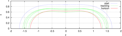
  Figure 8: CE surfaces with decreasing expansions $\lambda$ are tracked during a pseudo-evolution of Brill–Lindquist data until an apparent horizon is found. Each surface lives in a different spacelike hypersurface corresponding to a different “time”, where the black holes are in different locations. (Note the directions of the coordinate axes.)

  Table 7: Parameters of the tracked CE surfaces shown in figure 8. $\pm z$ are the coordinate locations of the two singularities, $\lambda$ is the expansion of the CE surface, $R$ its areal radius. For $\lambda=0$, $R/2$ is the irreducible mass.

  • $z$	$\lambda$	$R$	$R/2$
    $1.00$	$0.07$	$3.97820$	$1.98910$
    $0.95$	$0.05$	$3.92198$	$1.96099$
    $0.90$	$0.04$	$3.93548$	$1.96774$
    $0.85$	$0.03$	$3.94254$	$1.97127$
    $0.80$	$0.01$	$3.93648$	$1.96824$
    $0.75$	$0.00$	$3.95218$	$1.97609$

  6 Summary

  Apparent horizons and other CE surfaces provide valuable insight into spacetimes that are given numerically. Apparent horizons provide mass and spin estimates for black holes; they are indicators for event horizons, and help keep track of the location of singularities. CE surfaces are a generalisation of apparent horizons. Empirically, they lead to a foliation of a spacelike hypersurface outside a small interior region. They can be used to compare spacetimes that are given in different coordinate systems (but with the same slicing), and provide a measure for the coordinate distortions of the three-metric.

  The presented CE surface finding algorithm provides an efficient and robust way to find apparent horizons and other CE surfaces, and also a fast way to track CE surfaces during a numerical evolution, helping to find new apparent horizons as they appear.

References

- [1] Abhay Ashtekar, Christopher Beetle, Olaf Dreyer, Stephen Fairhurst, Badri Krishnan, Jerzy Lewandowski, and Jacek Wiśniewski. Generic isolated horizons and their applications. Phys. Rev. Lett., 85:3564–3567, 2000.
- [2] Abhay Ashtekar, Christopher Beetle, and Jerzy Lewandowski. Mechanics of rotating isolated horizons. Phys. Rev. D, 64:044016, 2001.
- [3] Olaf Dreyer, Badri Krishnan, Deirdre Shoemaker, and Erik Schnetter. Introduction to isolated horizons in numerical relativity. Phys. Rev. D, 67:024018, January 2003.
- [4] Jonathan Thornburg. Finding apparent horizons in numerical relativity. Phys. Rev. D, 54:4899–4918, 1996.
- [5] M. Alcubierre, S. Brandt, B. Brügmann, C. Gundlach, J. Massó, E. Seidel, and P. Walker. Test-beds and applications for apparent horizon finders in numerical relativity. Class. Quantum Grav., 17:2159–2190, 2000.
- [6] Gerhard Huisken and Shing-Tung Yau. Definition of the center of mass for isolated physical systems and unique foliations by stable spheres with constant mean curvature. Invent. Math., 1:281–311, 1996.
- [7] Thomas W. Baumgate and Stuart L. Shapiro. Numerical relativity and compact binaries. Phys. Rep., 376:41–131, 2003.
- [8] M. Shibata and K. Uryū. Apparent horizon finder for general three-dimensional spaces. Phys. Rev. D, 62:087501, 2000.
- [9] Mijan F. Huq, Matthew W. Choptuik, and Richard A. Matzner. Locating boosted Kerr and Schwarzschild apparent horizons. gr-qc/0002076, 2000.
- [10] Deirdre M. Shoemaker, Mijan F. Huq, and Richard A. Matzner. Generic tracking of multiple apparent horizons with level flow. Phys. Rev. D, 62:124005, 2000.
- [11] Takashi Nakamura, Yasufumi Kojima, and Ken ichi Oohara. A method of determining apparent horizons in three dimensional numerical relativity. Phys. Lett. A, 106:235–238, 1984.
- [12] Thomas W. Baumgarte, Gregory B. Cook, Mark A. Scheel, Stuart L. Shapiro, and Saul A. Teukolsky. Implementing an apparent-horizon finder in three dimensions. Phys. Rev. D, 54:4849–4857, 1996.
- [13] Carsten Gundlach. Pseudo-spectral apparent horizon finders: an efficient new algorithm. Phys. Rev. D, 57:863–875, 1998.
- [14] P. Anninos, K. Camarda, J. Libson, J. Massó, E. Seidel, and W.-M. Suen. Finding apparent horizons in dynamic 3D numerical spacetimes. Phys. Rev. D, 58:024003, 1998.
- [15] Jonathan Thornburg. A fast apparent-horizon finder for 3-dimensional Cartesian grids in numerical relativity. gr-qc/0306056, 2003.
- [16] Harry Yserentant. Hierarchical bases. In R. E. O’Malley, editor, ICIAM 91, pages 256–276, Washington, DC, 1992. SIAM, Philadelphia.
- [17] Gregory B. Cook and James W. York Jr. Apparent horizons for boosted or spinning black holes. Phys. Rev. D, 41(4):1077–1085, 1990.
- [18] Gregory B. Cook and Andrew M. Abrahams. Horizon structure of initial-data sets for axisymmetric two-black-hole collisions. Phys. Ref. D, 46(2):702–713, 1992.
- [19] M. Shibata. Apparent horizon finder for a special family of spacetimes in 3D numerical relativity. Phys. Rev. D, 55:2002, 1997.
- [20] Eberhard Pasch. The level set method for the mean curvature flow on (R3,g). Technical Report 63, SFB 382, SFB 382–Geschäftsstelle, Auf der Morgenstelle 10, 72076 Tübingen, Germany; Web: http://www.uni-tuebingen.de/uni/opx/projekte.html, 1997. Available online as http://www.uni-tuebingen.de/uni/opx/reports/pasch_63.ps.gz.
- [21] Cactus Authors. Cactus home page. http://www.cactuscode.org/, 2002.
- [22] Satish Balay, William D. Gropp, Lois C. MacInnes, and Barry F. Smith. PETSc home page. http://www.mcs.anl.gov/petsc, 1998.
- [23] Satish Balay, William D. Gropp, Lois C. McInnes, and Barry F. Smith. PETSc users manual. Technical Report ANL-95/11 - Revision 2.1.0, Argonne National Laboratory, 2000.
- [24] K. P. Tod. Looking for marginally trapped surfaces. Class. Quantum Grav., 8:L115–L118, 1991.
- [25] Gregory B. Cook. Initial data for numerical relativity. Living Reviews in Relativity, 3(5), 2000.
- [26] Steven Weinberg. Gravitation and Cosmology, chapter 6.6, page 165 ff. John Wiley and Sons, 1972.
- [27] Willy Krivan and Heinz Herold. 2-surfaces of constant mean curvature in physical spacetimes. Class. Quantum Grav., 12:2297–2308, 1995.
- [28] Dieter R. Brill. On the positive definite mass of the Bondi-Weber-Wheeler time-symmetric gravitational waves. Ann. Phys., 7:466–483, 1959.
- [29] Joan Massó, Edward Seidel, Wai-Mo Suen, and Paul Walker. Event horizons in numerical relativity. II. Analyzing the horizon. Phys. Rev. D, 59:064015, 1999.
- [30] Richard A. Mazner, Mijan F. Huq, and Deirdre Shoemaker. Initial data and coordinates for multiple black hole systems. Phys. Rev. D, 59:024015, 1999.
-