The relativistic Sagnac effect:
two derivations

Abstract

The phase shift due to the Sagnac Effect, for relativistic matter and electromagnetic beams, counter-propagating in a rotating interferometer, is deduced using two different approaches. From one hand, we show that the relativistic law of velocity addition leads to the well known Sagnac time difference, which is the same independently of the physical nature of the interfering beams, evidencing in this way the universality of the effect. Another derivation is based on a formal analogy with the phase shift induced by the magnetic potential for charged particles travelling in a region where a constant vector potential is present: this is the so called Aharonov-Bohm effect. Both derivations are carried out in a fully relativistic context, using a suitable 1+3 splitting that allows us to recognize and define the space where electromagnetic and matter waves propagate: this is an extended 3-space, which we call relative space. It is recognized as the only space having an actual physical meaning from an operational point of view, and it is identified as the ’physical space of the rotating platform’: the geometry of this space turns out to be non Euclidean, according to Einstein’s early intuition.

1 Introduction

The effects of rotation on space-time have always been sources of stimulating and fascinating physical issues for the last centuries. Indeed, even before the introduction of the concept of space-time continuum, the peculiarity of the rotation of the reference frame was recognized and understood. A beautiful example is the Foucault’s pendulum, which shows, in the context of Newtonian physics, the absolute character of rotation.

At the dawn of the modern scientific era, the notions of absolute space and time, which are fundamental in the formulation of classical laws of physics, were criticized by Leibniz[1] and Berkeley[2]; consequently, the concepts of absolute motion, and hence, of absolute rotation, were questioned too. Mach’s[3] analysis of the relativity of motions revived the debate at the dawn of Theory of Relativity. As it is well known, Mach’s ideas played an important role and influenced Einstein’s approach. However, the peculiarity of rotation, which is inherited by Newtonian physics, leads to bewildering problems even in the relativistic context. Actually, after the publication of Einstein’s theory, those who were prejudicely contrary to Relativity found, in the relativistic approach to rotation, important arguments against the self-consistency of the theory. In 1909 an apparent logical contradiction in the Special Theory of Relativity (SRT), applied to the case of a rotating disk, was pointed out by Ehrenfest[4]. Subsequently, in 1913, Sagnac[5] evidenced an apparent contradiction in the SRT with respect to experiments performed with rotating interferometers: according to him

L’effet interférentiel observé […] manifeste directment l’existence de l’éther, support nécessaire des ondes lumineuses de Huygens et de Fresnel.

Since those years, both the so-called ’Ehrenfest’s paradox’ and the theoretical interpretation of the Sagnac effect have become topical arguments of a discussion on the foundations of the SRT, which is not closed yet, as the number of recent contributions confirms.

We studied elsewhere[6] the Ehrenfest’s paradox, and we showed that it can be solved on the basis of purely kinematical arguments in the SRT. In this paper we are concerned with the Sagnac effect: we are going to show that it can be completely explained in the SRT. To this end, we are going to give two derivations of the effect.

On the one hand, using relativistic kinematics and, namely, the law of velocity addition, we are going to provide a ”direct” derivation of the effect. In particular, the universality of the effect - i.e. its independence from the physical nature and the velocities (relative to the turntable) of the interfering beams - will be explained.

On the other hand, we are going to give a ”derivation by analogy” which generalizes a previous work written by Sakurai[7]. Indeed, Sakurai outlined a beautiful and far-reaching analogy between the Sagnac effect and the Aharonov-Bohm effect[8], and obtained a first order approximation of the Sagnac effect. By generalizing Sakurai’s result, we shall obtain the Sagnac effect in full theory, without any approximation, evidencing that the analogy holds also in a fully relativistic context. To this end, we shall use Cattaneo’s 1+3 splitting [9], [10], [11], [12], [13], that will enable us to describe the geometrodynamics of the rotating frame in a simple and powerful way: in particular, some Newtonian elements used by Sakurai will be generalized to a relativistic context.

The present paper is organized as follows: in Section 2 a historical review of the Sagnac effect is made; in Section 3 the direct derivation is given, while the derivation by analogy is outlined in Section 4. Finally, a thorough exposition of the foundations of Cattaneo’s splitting is given in Appendix.

2 A little historical review of the Sagnac effect

2.1 The early years

The history of the interferometric detection of the effects of rotation dates back to the end of the XIX century when, still in the context of the ether theory, Sir Oliver Lodge[14] proposed to use a large interferometer to detect the rotation of the Earth. Subsequently[15] he proposed to use an interferometer rotating on a turntable in order to reveal the rotation effects with respect to the laboratory frame. A detailed description of these early works can be found in the paper by Anderson et al.[16], where the study of rotating interferometers is analyzed in a historical perspective. In 1913 Sagnac[5] verified his early predictions[17], using a rapidly rotating light-optical interferometer. In fact, on the ground of classical physics, he predicted the following fringe shift (with respect to the interference pattern when the device is at rest), for monochromatic light waves in vacuum, counter-propagating along a closed path in a rotating interferometer:

$$\Delta z=\frac{4\mathbf{\Omega\cdot S}}{\lambda c}$$ (1)

where $\mathbf{\Omega}$ is the (constant) angular velocity vector of the turntable, $\mathbf{S}$ is the vector associated to the area enclosed by the light path, and $\lambda$ is the wavelength of light in vacuum (as seen in the local co-moving inertial frame of the light source). The time difference associated to the fringe shift (1) turns out to be

$$\Delta t=\frac{\lambda}{c}\Delta z=\frac{4\mathbf{\Omega\cdot S}}{c^{2}}$$ (2)

Even if his interpretation of these results was entirely in the framework of the classical (not Lorentz’s!) ether theory, Sagnac was the first scientist who reported an experimental observation of the effect of rotation in space-time, which, after him, was named ”Sagnac effect”. It is noteworthy to notice that the Sagnac effect has been interpreted as a disproval of the SRT since the early years of relativity (in particular by Sagnac himself) up to now (in particular by Selleri[18],[19], Croca-Selleri[20], Goy-Selleri[21], Vigier[22], Anastasowski et al.[23], Klauber[24],[25]). However, this claim is incorrect. As a matter of fact, the Sagnac effect can be completely explained in the framework of the SRT: see for instance Weber[26], Dieks[27], Anandan[28], Rizzi-Tartaglia[29], Bergia-Guidone [30], Rodrigues-Sharif[31], Pascual-Sánchez et al.[32]. According to the SRT, eq. (2) turns out to be just a first order approximation of the relativistic proper time difference between counter-propagating light beams. Moreover, in what follows, it will be apparent that the relativistic interpretation of the Sagnac effect allows a deeper insight into the very foundations of the SRT.

Few years before Sagnac, Franz Harres[33], graduate student in Jena, observed (for the first time but unknowingly) the Sagnac effect during his experiments on the Fresnel-Fizeau drag of light. However, only in 1914, Harzer[34] recognized that the unexpected and inexplicable bias found by Harres was nothing else than the manifestation of the Sagnac effect. Moreover, Harres’s observations also demonstrated that the Sagnac fringe shift is unaffected by refraction: in other words, it is always given by eq. (1), provided that $\lambda$ is interpreted as the light wavelength in a co-moving refractive medium. So, the Sagnac phase shift depends on the light wavelength, and not on the velocity of light in the (co-moving) medium.

If Harres anticipated the Sagnac effect on the experimental ground, Michelson[35] anticipated the effect on the theoretical side. Subsequently, in 1925, Michelson himself and Gale[36] succeeded in measuring a phase shift, analogous to the Sagnac’s one, caused by the rotation of the Earth, using a large optical interferometer.

The field of light-optical Sagnac interferometry had a revived interest after the development of laser (see for instance the beautiful review paper by Post[37], where the previous experiments are carefully described and their theoretical implications analyzed). After that, there was an increasing precision in measurements and a growth of technological applications, such as inertial navigation[38], where the ”fiber-optical gyro”[39] and the ”ring laser”[40] are used.

2.2 Universality of the Sagnac Effect

The experimental data show that: (i) the Sagnac fringe shift (1) does not depend either on the presence of a co-moving optical medium or on the group velocity of the counter-propagating beams; (ii) the Sagnac time difference (2) does not depend either on the light wavelength or on the presence of a co-moving optical medium. This is a first important clue of the universality of the Sagnac effect. However, the most compelling claim for the universal character of the Sagnac effect comes from the validity of eq. (1) not for light beams only, but also for any kind of ”entities” (such as electromagnetic and acoustic waves, classical particles and electron Cooper pairs, neutron beams and De Broglie waves and so on…) travelling in opposite directions along a closed path in a rotating interferometer, with the same (in absolute value) velocity with respect to the turntable. This fact is well proved by experimental texts (see Subsection 2.3).

Of course the entities take different times for a complete round-trip, depending on their velocity relative to the turntable; but the difference between these times is always given by eq. (2).  So, the amount of the time difference is always the same, both for matter and light waves, independently of the physical nature of the interfering beams.

This astounding but experimentally well proved ”universality” of the Sagnac effect is quite inexplicable on the basis of the classical physics, and invokes a geometrical explanation in the Minkowskian space-time of the SRT.

2.3 Experimental tests and derivation of the Sagnac Effect

The Sagnac effect with matter waves has been verified experimentally using Cooper pairs[41] in 1965, using neutrons[42] in 1984, using ${}^{40}Ca$ atoms beams[43] in 1991 and using electrons, by Hasselbach-Nicklaus[44], in 1993. The effect of the terrestrial rotation on neutron phase was demonstrated in 1979 by Werner et al.[45] in a series of famous experiments.

The Sagnac phase shift has been derived, in the full framework of the SRT, for electromagnetic waves in vacuum (Weber[26], Dieks[27], Anandan[28], Rizzi-Tartaglia[29], Bergia-Guidone [30], Rodrigues-Sharif[31]). However, a clear and universally shared derivation for matter waves is not available as far as we know, or it is at least difficult to find it in the literature. Indeed, the Sagnac phase shift for matter waves has been derived, in the first order approximation with respect to the velocity of rotation of the interferometer, by many authors (see Ashby’s paper in this book[46] and the paper by Hasselbach-Nicklaus for discussions and further references). These derivations are often based on an heterogeneous mixture of classical kinematics and relativistic dynamics, or non relativistic quantum mechanics and some relativistic elements.

An example of such derivations is given in a well known paper by Sakurai[7], on the basis of a formal analogy between the classical Coriolis force

$$\mathbf{F}_{Cor}=2m_{o}\mathbf{v}\times\mathbf{\Omega\;,}$$ (3)

acting on a particle of mass $m_{o}$ moving in a uniformly rotating frame, and the Lorentz force

$$\mathbf{F}_{Lor}=\frac{e}{c}\mathbf{v}\times\mathbf{B}$$ (4)

acting on a particle of charge $e$ moving in a constant magnetic field $\mathbf{B}$.

Sakurai considers a beam of charged particles split into two different paths and then recombined. If $S$ is the surface domain enclosed by the two paths, the resulting phase difference in the interference region turns out to be

$$\Delta\Phi=\frac{e}{c\hbar}\int_{S}\mathbf{B}\cdot\mathrm{d}\mathbf{S}$$ (5)

Therefore, $\Delta\Phi$ is different from zero when a magnetic field exists inside the domain enclosed by the two paths, even if the magnetic field felt by the particles along their paths is zero. This is the well known Aharonov-Bohm[8] effect. By formally substituting

$$\frac{e}{c}\mathbf{B}\rightarrow 2m_{o}\mathbf{\Omega}$$ (6)

Sakurai shows that the phase shift (5) reduces to

$$\Delta\Phi=\frac{2m_{o}}{\hbar}\int_{S}\mathbf{\Omega}\cdot d\mathbf{S}$$ (7)

If $\mathbf{\Omega}$ is interpreted as the angular velocity vector of the uniformly rotating turntable and $\mathbf{S}$ as the vector associated to the area enclosed by the closed path along which the two counter-propagating material beams travel, then eq. (7) can be interpreted as the Sagnac phase shift for the considered counter-propagating beams:

$$\Delta\Phi=\frac{2m_{o}}{\hbar}\mathbf{\Omega}\cdot\mathbf{S}$$ (8)

This result has been obtained using non relativistic quantum mechanics: the relations between the Aharonov-Bohm effect and the wave equations are discussed in Subsection 4.1.

The time difference corresponding to the phase difference (8), turns out to be:

$$\Delta t=\frac{\Delta\Phi}{\omega}=\frac{\hbar}{E}\Delta\Phi=\frac{\hbar}{mc^{2}}\Delta\Phi=\frac{2m_{o}}{mc^{2}}\mathbf{\Omega}\cdot\mathbf{S}$$ (9)

Let us point out that eq. (9) contains, inconsistently but unavoidably, some relativistic elements ($\hbar\omega=E=mc^{2}$). Of course in the first order approximation, i.e. when the relativistic mass $m$ coincides with the rest mass $m_{o}$, eq. (9) reduces to eq. (2); that is, as we stressed before, a first order approximation of the relativistic time difference associated to the Sagnac effect.

This simple and beautiful procedure will be generalized and extended to a fully relativistic context in Sec. 4.

3 Direct derivation: Sagnac effect for material and light particles

3.1 Direct derivation

In this section we are going to give a description of light or matter beams counter-propagating in a rotating interferometer, based on relativistic kinematics; here and henceforth, we shall refer to both light and matter beams by calling them simply ”beams”. Indeed, it is our aim to show that, under suitable conditions, the Sagnac time difference does not depend on the very physical nature of the interfering beams.

The beams are constrained to travel a circular path along the rim of the rotating disk, with constant angular velocity, in opposite directions. Let us suppose that a beam source and an interferometric detector are lodged on a point $\Sigma$ of the rim of the disk. Let $K$ be the central inertial frame, parameterized by an adapted (see Appendix A.6) set of cylindrical coordinates $\left\{x^{\mu}\right\}~{}=~{}\left(t,r,\vartheta,z\right)$, with line element given by

$$\mathrm{d}s^{2}=g_{\mu\nu}dx^{\mu}dx^{\nu}=-c^{2}\mathrm{d}t^{2}+\mathrm{d}r^{2}+r^{2}\mathrm{d}\vartheta^{2}+\mathrm{d}z^{2}\mathrm{\ }$$ (10)

In particular, if we confine ourselves to a the disk ($z=const$), the metric turns out to be

$$ds^{2}=-c^{2}dt^{2}+dr^{2}+r^{2}d\vartheta^{2}$$ (11)

With respect to $K$, the disk (whose radius is $R$) rotates with angular velocity $\Omega$, and the world-line $\gamma_{\Sigma}$ of $\Sigma$ is

$$\gamma_{\Sigma}\equiv\left\{\begin{array}[]{rcl}x^{0}&=&ct\\ x^{1}&=&r=R\\ x^{2}&=&\vartheta=\Omega t\end{array}\right.$$ (12)

or, eliminating $t$

$$\gamma_{\Sigma}\equiv\left\{\begin{array}[]{rcl}x^{0}&=&\frac{c}{\Omega}\vartheta\\ x^{1}&=&R\\ x^{2}&=&\vartheta\end{array}\right.$$ (13)

The proper time read by a clock at rest in $\Sigma$ is given by

$$\tau=\frac{1}{c}\int_{\gamma_{\Sigma}}|ds|=\frac{1}{c}\int_{\gamma_{\Sigma}}\sqrt{c^{2}dt^{2}-R^{2}d\vartheta^{2}}=\frac{1}{\Omega}\sqrt{1-\beta^{2}}\int_{\gamma_{\Sigma}}d\vartheta$$ (14)

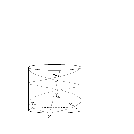
Figure 1: The world-line of $\Sigma$ (a point on the disk where a beam source and interferometric detector are lodged) is $\gamma_{\Sigma}$; $\gamma_{+}$ and $\gamma_{-}$ are the world-lines of the co-propagating (+) and counter-propagating (-) beams. The first intersection of $\gamma_{+}$ ($\gamma_{-}$) with $\gamma_{\Sigma}$ takes place at the time $\tau_{+}$ ($\tau_{-}$), as measured by a clock at rest in $\Sigma$.

The world-lines of the co-propagating (+) and counter-propagating (-) beams emitted by the source at time $t=0$ (when $\vartheta=0$) are, respectively:

$$\gamma_{+}\equiv\left\{\begin{array}[]{rcl}x^{0}&=&\frac{c}{\omega_{+}}\vartheta\\ x^{1}&=&R\\ x^{2}&=&\vartheta\end{array}\right.$$ (15)

$$\gamma_{-}\equiv\left\{\begin{array}[]{rcl}x^{0}&=&\frac{c}{\omega_{-}}\vartheta\\ x^{1}&=&R\\ x^{2}&=&\vartheta\end{array}\right.$$ (16)

where $\omega_{+},\omega_{-}$ are their angular velocities, as seen in the central inertial frame. The first intersection of $\gamma_{+}$ ($\gamma_{-}$) with $\gamma_{\Sigma}$ is the event ”absorption of the co-propagating (counter-propagating) beam after a complete round trip” (see figure 1).

This event takes place when

$$\frac{1}{\Omega}\vartheta_{\pm}=\frac{1}{\omega_{\pm}}(\vartheta_{\pm}\pm 2\pi)$$ (17)

where the $+$ ($-$) sign holds for the co-propagating (counter-propagating) beam. The solution of eq. (17) is:

$$\vartheta_{\pm}=\pm\frac{2\pi\Omega}{\omega_{\pm}-\Omega}$$ (18)

If we introduce the dimensionless velocities $\beta=\Omega R/c$, $\beta_{\pm}=\omega_{\pm}R/c$, the $\vartheta$-coordinate of the absorption event can be written as follows:

$$\vartheta_{\pm}=\pm\frac{2\pi\beta}{\beta_{\pm}-\beta}$$ (19)

Taking into account eq. (14), the proper time elapsed between the emission and the absorption of the co-propagating (counter-propagating) beam, read by a clock at rest in $\Sigma$, is given by

$$\tau_{\pm}=\ \ \pm\frac{2\pi\beta}{\Omega}\frac{\sqrt{1-\beta^{2}}}{\beta_{\pm}-\beta}$$ (20)

and the proper time difference $\Delta\tau\equiv\tau_{+}-\tau_{-}$ turns out to be

$$\Delta\tau=\frac{2\pi\beta}{\Omega}\sqrt{1-\beta^{2}}\frac{\beta_{-}-2\beta+\beta_{+}}{(\beta_{+}-\beta)(\beta_{-}-\beta)}$$ (21)

Without specifying any conditions, the proper time difference (21) appears to depend upon $\beta,\beta_{+},\beta_{-}$: this means that it does depend, in general, both on the velocity of rotation of the disk and on the velocities of the beams. Let $\beta_{\pm}^{\prime}$ be the velocities of the beams as measured in any Minkowski inertial frame, locally co-moving with the rim of the disk, or briefly speaking in any locally co-moving inertial frame (LCIF). Provided that each LCIF is Einstein-synchronized (see Subsection 3.5 below), the Lorentz law of velocity addition gives the following relations between $\beta_{\pm}^{\prime}$ and $\beta_{\pm}$:

$$\beta_{\pm}=\frac{\beta_{\pm}^{\prime}+\beta}{1+\beta_{\pm}^{\prime}\beta}$$ (22)

By substituting (22) in (21) we easily obtain

$$\Delta\tau=\frac{4\pi\beta^{2}}{\Omega}\frac{1}{\sqrt{1-\beta^{2}}}+\frac{2\pi\beta}{\Omega}\frac{1}{\sqrt{1-\beta^{2}}}\left(\frac{1}{\beta_{+}^{\prime}}+\frac{1}{\beta_{-}^{\prime}}\right)$$ (23)

Now, let us impose the condition ”equal relative velocity in opposite directions”:

$$\beta_{+}^{\prime}=-\beta_{-}^{\prime}$$ (24)

This condition means that the beams are required to have the same velocity (in absolute value) in every LCIF, provided that every LICF is Einstein-synchronized. If condition (24) is imposed, the proper time difference (23) reduces to

$$\Delta\tau=\frac{4\pi\beta^{2}}{\Omega}\frac{1}{\sqrt{1-\beta^{2}}}=\frac{4\pi R^{2}\Omega}{c^{2}}\left(1-\frac{\Omega^{2}R^{2}}{c^{2}}\right)^{-1/2}$$ (25)

which is the relativistic Sagnac time difference.

A very relevant conclusion follows. According to eq. (20), the beams take different times - as measured by the clock at rest on the starting-ending point $\Sigma$ on the platform - for a complete round trip, depending on their velocities $\beta_{\pm}^{\prime}$ relative to the turnable. However, when condition (24) is imposed, the difference $\Delta\tau$ between these times does depend only on the angular velocity $\Omega$ of the disk, and it does not depend on the velocities of propagation of the beams with respect the turnable.

This is a very general result, which has been obtained on the ground of a purely kinematical approach. The Sagnac time difference (25) applies to any couple of (physical or even mathematical) entities, as long as a velocity with respect the turnable can be consistently defined. In particular, this result applies as well to photons (for which $|\beta_{\pm}^{\prime}|=1$) and to any kind of classical or quantum particles under the given conditions (or electromagnetic/acustic waves in presence of an homogeneous co-moving medium). This fact highlights, in a clear and straightforward way, the universality of the Sagnac effect.

More in particular, the Sagnac time difference (25) also applies to the Fourier components of the wave packets associated to a couple of matter beams counter-propagating (with the same relative velocity) along the rim. This remark is important to study the interferometric detectability of the Sagnac effect (see Subsection 3.3 below).

3.2 The Sagnac effect as an empirical evidence of the SRT

As we said in the Introduction, the Sagnac effect for electromagnetic waves in vacuum was first interpreted by Sagnac himself as an experimental evidence of the physical existence of the classical (non relativistic) ether, and an experimental disproval of the SRT. Sagnac’s interpretation can be easily understood, on the basis of the relativistic eq. (21), as a casual consequence of a well known kinematical feature of light propagation through the ether. Indeed, the light velocity with respect to the ether (at rest in the central IF) must be $c$ in both directions; as a consequence, if we set $\beta_{\pm}=\pm 1$ in eq. (21), the proper time difference $\Delta\tau$ reduces to eq. (25); the latter, in turn, reduces, at first order approximation, to the time difference given in eq. (2), which was actually predicted and experimentally tested by Sagnac.

However, any non relativistic explanation completely fails for subluminally travelling entities (such as matter waves, sound waves, electromagnetic waves in an homogeneous co-moving medium, and so on). In fact, for subluminally travelling entities the vital condition is: ”equal relative velocity in opposite directions”. If this condition is expressed by eq. (24) (which explicitly requires the local Einstein synchronization) the Sagnac proper time difference (25) arises, as we carefully showed before.

On the contrary, if the condition ”equal relative velocity in opposite directions” is expressed by an analogous relation, in which the local Einstein synchronization is replaced by a synchronization borrowed from the global synchronization of the central IF (see Subsection 3.5), no time difference arises. Let us prove this claim.

Let $\varphi_{\pm}$ and $\vartheta_{\pm}^{r}$ be the azimuthal coordinates of the co-rotating/counter-rotating entity with respect to the central IF and the LCIF, respectively. These coordinates are related by the transformation

$$\varphi_{\pm}=\Omega t+\vartheta^{r}_{\pm}$$ (26)

Derivation of eq. (26) with respect to the central inertial time $t$ gives

$$\omega_{\pm}=\Omega+\omega_{\pm}^{r}$$ (27)

where $\omega_{\pm}\equiv d\varphi_{\pm}/dt$ is the angular velocity relative to the central IF, and $\omega_{\pm}^{r}\equiv d\vartheta_{\pm}^{r}/dt$ is the angular velocity relative to the LCIF - provided that it is synchronized by means of the central inertial time $t$.

Eq. (27), multiplied by R/c, takes the dimensionless form

$$\beta_{\pm}=\beta+\beta_{\pm}^{r}$$ (28)

which replaces eq. (22). Let us stress that both eqs. (22) and (28) are correct: the former refers to the local Einstein synchronization, the latter to the local synchronization according to the simultaneity criterium of the central IF.

Introducing eq. (28) into eq. (21), the proper time difference $\Delta\tau$ reduces to

$$\Delta\tau=\frac{2\pi\beta}{\Omega}\sqrt{1-\beta^{2}}\frac{(\beta+\beta_{-}^{r})-2\beta+(\beta+\beta_{+}^{r})}{\beta_{-}^{r}\beta_{+}^{r}}=\frac{2\pi\beta}{\Omega}\sqrt{1-\beta^{2}}\frac{\beta_{-}^{r}+\beta_{+}^{r}}{\beta_{-}^{r}\beta_{+}^{r}}$$ (29)

If the vital condition ”equal relative velocity in opposite directions” is expressed by eq.

$$\beta_{+}^{r}=-\beta_{-}^{r}$$ (30)

instead of eq. (24), it is plain from eq. (29) that no time difference arises: $\Delta\tau=0$ (Q.E.D.)

This calculation shows that the choice of the local Einstein synchronization is crucial even in non-relativistic motion. Indeed, the choice of the classical eq. (28), instead of the relativistic eq. (22), could be naively presumed as a reasonable approximation in non-relativistic motion: however, this choice simply cancels the effect!

This shows that, according to a very appropriate remark by Dieks and Nienhuis [47], the observed Sagnac effect is an experimental evidence of the SRT at first order approximation with respect to $\beta=\Omega R/c$, and an experimental disproval of the classical (non relativistic) ether.

Remark It could be always possible to substitute eq. (24) with an alternative suitable condition, so that eq. (29) turns out to be equal to eq. (25). Such a condition is:

$$\beta_{-}^{r}=-\beta_{+}^{r}\frac{1-\beta^{2}}{1-2\beta\beta_{+}^{r}-\beta^{2}}$$ (31)

But, of course, this is an extremely ”ad hoc” condition, which translates the simple and expressive condition (24): it is clear that the physical interpretation of (31) is not as evident as that of (24).

3.3 Interferometric detectability of the Sagnac effect

With regard to the interferometric detection of the Sagnac effect, the crucial point is the following one. Consider the Fourier components of the wave packets associated to a couple of matter beams counter-propagating, with the same group velocity, along the rim. Despite the lack of a direct physical meaning and energy transfer, the phase velocity of these Fourier components complies with the Lorentz law of velocity addition (22 ), and is the same for both the co-rotating and counter-rotating Fourier components. As a consequence, the Sagnac time difference (25) also applies to any couple of Fourier components with the same phase velocity.

Moreover, the interferometric detection of the Sagnac effect requires that the wave packet associated to the matter beam should be sharp enough in the frequency space, to allow the appearance, in the interferometric region, of an observable fringe shift. It may be worth recalling that:

(i) the observable fringe shift $\Delta z$ depends on the phase velocity of the Fourier components of the wave packet;

(ii) with respect to an Einstein-synchronized LCIF, the velocity of every Fourier component of the wave packet associated to the matter beam, moving with the velocity (in absolute value) $v\equiv c|\beta_{\pm}^{\prime}|$, is given by the De Broglie expression $v_{f}=c^{2}/v$.

The consequent Sagnac phase shift, due to the relativistic time difference (25), is

$$\Delta\Phi=2\pi\Delta z=2\pi\left(\frac{v_{f}}{\lambda}\Delta\tau\right)=\frac{8\pi^{2}R^{2}\Omega}{\lambda v}\left(1-\frac{\Omega^{2}R^{2}}{c^{2}}\right)^{-1/2}$$ (32)

3.4 Comparing to some results found in the literature

As we mentioned, the Sagnac time delay for matter beams has been derived by many authors in many different ways, but almost always in the first order approximation. However, digging into the literature, we eventually found, between the preliminary and the final version of this paper, a couple of derivations of the Sagnac effect for matter beams in full SRT. In this section we are going to compare these approaches to ours.

3.4.1 Dieks-Nienhuis’s approach

Dieks and Nienhuis[47] move from the standard Lorentz transformation from the LCIF to the central IF. In order to be as clear and self-consistent as possible, we shall translate everything into our notations.

Consider two near events, happening along the rim, belonging to the world-line of the co-rotating/counter-rotating beam; let $dx$, d$\tau$ be the space and time separation between these events, as measured in an Einstein-synchronized LCIF. Then the corresponding time separation $dt$, as measured in the central IF, is given by the usual Lorentz transformation

$$dt=\left(d\tau\pm\frac{\Omega Rdx}{c^{2}}\right)\left(1-\frac{\Omega^{2}R^{2}}{c^{2}}\right)^{-1/2}$$ (33)

where the $+$ and $-$ hold for the co-rotating and counter-rotating beams, respectively. Gluing together all LCIFs, at the end of the round trip we have

$$\left(1-\frac{\Omega^{2}R^{2}}{c^{2}}\right)^{1/2}t_{\pm}=\tau(\gamma_{\pm})\pm\frac{\Omega R}{c^{2}}\int_{D}dx$$ (34)

where $D$ is the length of the rim of the platform, as seen on the platform itself.

The difference between the equations for the co-rotating and counter-rotating beams is:

$$\left(1-\frac{\Omega^{2}R^{2}}{c^{2}}\right)^{1/2}(t_{+}-t_{-})=\tau(\gamma_{+})-\tau(\gamma_{-})+\frac{2\Omega R}{c^{2}}\int_{D}dx$$ (35)

In the derivation given by Dieks and Nienhuis, two hypotheses play a vital role in order to get the correct conclusion: (i) the integration domain $D$ is $2\pi R\left(1-\frac{\Omega^{2}R^{2}}{c^{2}}\right)^{-1/2};$ (ii) $\tau(\gamma_{+})=\tau(\gamma_{-})=\left(\frac{2\pi R}{v^{\prime}}\right)\left(1-\frac{\Omega^{2}R^{2}}{c^{2}}\right)^{-1/2},$ where $v^{\prime}$ is the relative velocity (in absolute value) of both the co-rotating and the counter-rotating beam (as a consequence, $\tau(\gamma_{+})-\tau(\gamma_{-})=0$).

Of course, the two hypotheses are correct, but both deserve further remarks. First of all, we could say that hypothesis (i) is unnecessary: indeed, our derivation of the Sagnac effect does not depend on the hyperbolic features of the space geometry of the disk (see Subsection 4.2 and Appendix A.14). On the other hand, this hypothesis establishes a very interesting link between the (observable) Sagnac time delay and the (unobservable) lengthening of the rim of the rotating platform, which, in turn, depends on the peculiar space geometry of the disk. This is a challenge to those authors (see for instance [25],[48]) who try to conciliate the Sagnac time delay with the Euclidean space geometry of the disk.

3.4.2 Malykin’s approach

The long review paper by Malykin[52] (almost 300 references!) starts with the remark that the Sagnac effect for matter beams ”is explained in several totally different ways”, but - strangely enough - most of them give ”correct results despite their obvious incorretness”. After a wide overview of these ”incorrect explanations”, the author provides his attempt of solution on the basis of the relativistic law of velocity addition. This approach is the only one that turns out to be similar to ours; also the problem of the interferometric detection of the Sagnac effect is taken into account. Of course, this leads to the issue of the kinematical behavior of both the phase velocity and the group velocity. Here some misinterpretations and confusions arise. In particular, the author tries to show that ”both the group velocity and the phase velocity have identical translational properties during the transition from the frame of reference K [the central IF] to the frame of reference K’ [the LCIF]”.

Actually, the group velocity behaves contrary to the phase velocity with respect to the (local) Lorentz transformation group. However, this has no consequences on the interferometric detection of the Sagnac effect, because the only relevant requirement is that, with respect to any Einstein-synchronized LCIF: (i) the group velocities should be the same; (ii) the phase velocities of the Fourier components should be the same. This is exactly what happens: the transformation properties have no role. Anyway, we agree with Malykin when he says that ”the Sagnac effect constitutes a kinematical effect of SRT; (…) all explanations of the Sagnac effect are incorrect except the relativistic one”. We agree also with his final remark: the existence of a large number of incorrect explanations which give correct results (at least in first approximation) depends on the fact that the Sagnac effect is a first-order effect in $v/c$.

3.4.3 Anderson, Stedman and Bilger’s approach

It is interesting to compare our results to this approach, even though Anderson, Stedman and Bilger’s results[40],[16] are confined to a first order approximation. Indeed, they find, at first order approximation, the following time difference:

$$\Delta t=\frac{4\mathbf{\Omega\cdot S}}{v^{2}}$$ (36)

and the following phase shift:

$$\Delta\Phi=\frac{8\pi\mathbf{\Omega\cdot S}}{\lambda v}$$ (37)

where $v$ is the ”undragged” velocity of the beams. Of course, the time difference (36) is not in agreement with the first order approximation (with respect to $\beta=\Omega R/c$) of eq. (25). However, it is consistent with the first order approximation of eq. (21) provided that $\beta_{+}=-\beta_{-}\equiv v/c$: this represents a completely different physical situation, in which the two beams are injected into the rotating platform (tangentially to the rim) in opposite directions with the same velocity with respect to the central inertial frame.

In addition, the phase shift (37), which is the only observable quantity through an interferometric device, is not in agreement with the physical situation considered by these authors. However, it is worthwhile to notice that, oddly enough, it perfectly agrees with the first order approximation of eq. (32).

3.4.4 Ashby’s approach

The best approach we know, at first order approximation, is the one suggested in this book by Ashby [46]. The peculiarity of this approach is that it is independent of the shape of the loop: this is a very important feature if one has to deal with the Global Positioning System (GPS). In particular, Ashby shows that the Sagnac time delay depends only on the area swept out by the electromagnetic pulse, as it travels from the GPS transmitter to the receiver, projected onto the terrestrial equatorial plane. A great care is devoted to synchronization problems: this issue is in complete agreement with our fully relativistic approach (see Subsection 3.5 below).

3.5 Synchronization in a LCIF: a free choice

As pointed out by Rizzi-Serafini[50], in a local or global inertial frame (IF) the synchronization is not ”given by God”, as often both relativistic and anti-relativistic authors assume, but it can be arbitrarily chosen within the synchronization gauge

$$\left\{\begin{array}[]{l}t^{\prime}=t^{\prime}\,(\,t,\,x^{1},x^{2},x^{3})\\ x_{i}^{\prime}=x_{i}\end{array}\right.$$ (38)

The synchronization gauge (38) is a subset of the Cattaneo gauge (56) (see Appendix A.4), which is the set of all possible parameterizations of the given physical inertial frame (IF). In eq. (38) the coordinates ($t,x_{i}$) are Einstein coordinates, and ($t^{\prime},x_{i}^{\prime}$) are re-synchronized coordinates of the IF under consideration. Of course, the IF turns out to be optically isotropic if and only if it is parameterized by Einstein coordinates ($t,x_{i}$). Then the following question arises: if the parameterization (in particular the synchronization) of a LCIF is a matter of choice, which is the most profitable choice in order to describe the Sagnac effect?

Since the synchronization gauge (38) is too general for a clear and useful discussion, it is advantageous to introduce a suitable subset of the synchronization gauge that allows a clearer discussion. Such a sub-gauge actually exists; it has been introduced by Selleri[18],[19]. Let us briefly summarize the so-called ”Selleri gauge”.

Let $K$ be a ”formally privileged” IF, in which an isotropic synchronization (that is Einstein synchronization) is assumed by stipulation; and let $S$ be a (generally anisotropic) IF moving along the $x_{1}^{\prime}=x_{1}$ axis with dimensionless velocity $\beta$ with respect to $K$. The Selleri gauge is defined by

$$\left\{\begin{array}[]{l}t^{\prime}=t+\frac{\Gamma(\beta)}{c}x\\ x_{i}^{\prime}=x_{i}\end{array}\right.$$ (39)

where the unprimed coordinates refer to the Einstein-synchronized IF $K$, the primed coordinates refer to the arbitrarily-synchronized IF $S$ and $\Gamma(\beta)$ is an arbitrary function of $\beta$. It is convenient to write this function as follows:

$$\Gamma(\beta)\equiv\beta+e_{1}(\beta)c\gamma^{-1}$$ (40)

The function $e_{1}(\beta)$ is Selleri’s ”synchronization parameter”, which, in principle, can be arbitrarily chosen. Any choice of the function $e_{1}(\beta)$ is a choice of the synchronization in the IF under consideration; in principle, the synchronization can be freely chosen inside the Selleri gauge (39). In particular, the synchrony choice $e_{1}(\beta)\doteq-\beta\gamma/c$ (i.e. $\Gamma(\beta)\doteq 0$) gives the standard Einstein synchronization, which is ”relative” (that is, frame-dependent); whereas the synchrony choice $e_{1}(\beta)\doteq 0$ gives the Selleri synchronization, which is ”absolute” (that is, frame-independent).

The term ”absolute” sounds rather eccentric in a relativistic framework, but it simply means that the Selleri simultaneity hypersurfaces $t^{\prime}=const$ (contrary to the Einstein simultaneity hypersurfaces $t=const$) define a frame-invariant foliation of space-time - which is nothing but the Einstein foliation of the particular IF $K$ assumed (by stipulation, once and for all) as optically isotropic for any choice of the synchronization parameter.

According to Selleri, the synchronization is a matter of convention in the case of translation, but not in the case of rotation: when rotation is taken into account, the synchronization parameter $e_{1}$ is forced to take the value zero. On the contrary, as it is shown in [50], the choice of $e_{1}$ is not compelled by any empiric evidence: that is, also when rotation is taken into account, no physical effect can discriminate  Selleri’s synchrony choice $e_{1}(\beta)\doteq 0$ from the Einstein’s synchrony choice $e_{1}(\beta)\doteq-\beta\gamma/c$.

Therefore, we have the opportunity of taking a very pragmatic view: both Selleri ”absolute” synchronization and Einstein relative synchronization can be used, depending on the aims and circumstances. In particular, (i) if we look for a global synchronization on the rotating platform, Selleri ”absolute” synchronization is required; (ii) if we look for a plain kinematical relationship between local velocities, Einstein synchronization is required in any LCIF.

Let us outline the advantages of the local Einstein synchronization on a rotating platform. First, let us recall[50] that the local isotropy or anisotropy of the velocity of light in a LCIF is not a fact, with a well defined ontological meaning, but a convention which depends on the synchronization chosen in the LCIF. Of course the velocity of light has the invariant value $c$ in every LCIF, both in co-rotating and counter-rotating direction, if and only if the LCIFs are Einstein-synchronized. We are aware that this statement sounds irrelevant or arbitrary to some authors[24], [18], [19], [53], so we try to suggest a more significant one. As we showed in Subsection. 3.1, the Sagnac time difference (25) holds for two beams travelling along the rim in opposite directions with the same velocity with respect the turnable. This is a plain and meaningful condition: but it must be stressed that this condition requires that every LCIF should be Einstein-synchronized. Of course this condition could be translated also into Selleri absolute synchronization, but it would result in a very artificial and convoluted requirement, namely eq. (31). Only Einstein synchronization allows the clear and meaningful requirement: ”equal relative velocity in opposite directions”.

4 The Sagnac effect from an analogy with the Aharonov-Bohm effect

In this section we shall give another derivation of the Sagnac effect for relativistic material beams counter-propagating on a rotating disk[54]. This derivation is based on a (formal) analogy with the Aharonov-Bohm effect which has been outlined by Sakurai[7]. However, Sakurai’s approach, which rests upon the use of relativistic and Newtonian elements, gives only the first order approximation of Sagnac time difference (25). We want to show that, using Cattaneo’s splitting techniques, it is possible to state the analogy between the Aharonov-Bohm effect and the Sagnac effect in a fully relativistic context, getting rid of the Newtonian elements and recovering the relativistic self-consistency of the derivation. On equal footing, our approach allows us to obtain the Sagnac time difference in full theory and not in its first order approximation, to which Sakurai and other authors confined themselves, exploiting the analogy with the Aharonov-Bohm effect.

According to us, our derivation highlights the common geometric nature of the two effects, which is the basis of their far-reaching analogy.

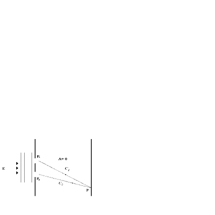
Figure 2: A single coherent charged beam, originating in $E$, is split into two parts (passing through the two slits $F_{1}$ and $F_{2}$) that propagate, respectively, along the paths $C_{1}$ and $C_{2}$ (in the figure these paths are represented, respectively, by $EF_{1}P$ and $EF_{2}P$). The beams travel in a region where a vector potential $\mathbf{A}$ is present. In $P$, the beams interfere and an additional phase shift is provoked by the magnetic field.

4.1 The Aharonov-Bohm effect

Let us start by briefly describing the Aharonov-Bohm effect. Consider the two slits experiment (figure 2) and imagine that a single coherent charged beam is split into two parts, which travel in a region where only a magnetic field is present, described by the 3-vector potential ${\bf A}$; then the beams are recombined to observe the interference pattern. The phase of the two wave functions, at each point of the pattern, is modified, with respect to the case of free propagation (${\bf A}~{}=~{}0$), by the magnetic potential. The magnetic potential-induced phase shift has the form[8]

$$\Delta\Phi=\frac{e}{c\hbar}\oint_{C}{\bf A}\cdot{\rm d}{\bf r}=\frac{e}{c\hbar}\int_{S}{\bf B}\cdot{\rm d}{\bf S}$$ (41)

where $C$ is the oriented closed curve, obtained as the sum of the oriented paths $C_{1}$ and $C_{2}$ relative to each component of the beam (in the physical space, see figure 2). Eq. (41) expresses (by means of Stoke’s Theorem) the phase difference in terms of the flux of the magnetic field across the surface $S$ enclosed by the curve $C$. Aharonov and Bohm[8] applied this result to the situation in which the two split beams pass one on each side of a solenoid inserted between the paths (see figure 3). Thus, even if the magnetic field ${\bf B}$ is totally contained within the solenoid and the beams pass through a ${\bf B}~{}=~{}0$ region, a resulting phase shift appears, since a non null magnetic flux is associated to every closed path which encloses the solenoid.

Tourrenc[55] showed that no explicit wave equation is demanded to describe the Aharonov-Bohm effect, since its interpretation is a pure geometric one: in fact eq. (41) is independent of the nature of the interfering charged beams, which can be spinorial, vectorial or tensorial. So, if we deal with relativistic charged beams, their propagation is described by a relativistic wave equation, such as the Dirac equation or the Klein-Gordon equation, depending on the nature of the beams themselves . From a physical point of view, spin has no influence on the Aharonov-Bohm effect because there is no coupling with the magnetic field which is confined inside the solenoid. Moreover, if the magnetic field is null, the Dirac equation is equivalent to the Klein-Gordon equation, and this is the case of a constant potential. As far as we are concerned, since in what follows we neglect spin, we shall just use eq. (41) and we shall not refer explicitly to any relativistic wave equation.

Indeed, things are different when a particle with spin moving in a rotating frame is considered. In this case a coupling between the spin and the angular velocity of the frame appears (this effect is evaluated by Hehl-Ni[56], Mashhoon[57] and Papini[58]).

Hence, the formal analogy that we are going to outline between matter waves moving in a uniformly rotating frame, and charged beams moving in a region where a constant magnetic potential is present, holds only when the spin-rotation coupling is neglected.

4.2 The relative space of a rotating disk

Before going on with our ”demonstration by analogy”, we want to recall the definition of the ”relative space” of a rotating disk, that we introduced elsewhere[6]. Since our analogy with the Aharonov-Bohm effect is based on the measurements performed by the observers on the disk, the concept of relative space is necessary to define, in a proper mathematical way, the physical context in which measurements are made. Even though a global isotropic 1+3 splitting of the space-time is not possible when we deal with rotating observers (see Appendix A.8 and A.14), the introduction of the relative space allows well defined procedures for the space and time measurements that can be performed (at large) by the observers in rotating frames, and which reduce to the standard space and time measurements locally (that is, in every Einstein-synchronized LCIF). Let us outline the main points that lead to the definition of the relative space.

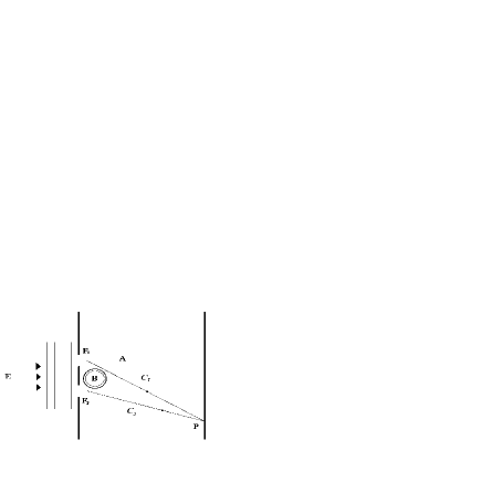
Figure 3: A single coherent charged beam, originating in $E$, is split into two parts (passing through the two slits $F_{1}$ and $F_{2}$) that propagate, respectively, along the paths $C_{1}$ and $C_{2}$ (in the figure these paths are represented, respectively, by $EF_{1}P$ and $EF_{2}P$). Between the paths a solenoid is present; the magnetic field $\mathbf{B}$ is entirely contained inside the solenoid, while outside there is a constant vector potential $\mathbf{A}$. In $P$, the beams interfere and an additional phase shift, provoked by the magnetic field confined inside the solenoid, is observed.

The world-lines of each point of the rotating disk are time-like helixes (whose pitch, depending on $\Omega$, is constant), wrapping around the cylindrical surface $r~{}=~{}const$, with $r\in[0,R]$. These helixes fill, without intersecting, the whole space-time region defined by $r\leq R<c/\Omega$; they constitute a time-like congruence $\Gamma$ which defines the rotating frame $K_{rot}$, at rest with respect to the disk. Let us introduce the coordinate transformation

$$\left\{\begin{array}[]{rcl}x^{\prime 0}&=&ct^{\prime}=ct\\ x^{\prime 1}&=&r^{\prime}=r\\ x^{\prime 2}&=&\vartheta^{\prime}=\vartheta-\Omega t\\ x^{\prime 3}&=&z^{\prime}=z\end{array}\right.\mathrm{\ .}$$ (42)

The coordinate transformation $\left\{x^{\mu}\right\}\rightarrow\left\{x^{\prime\mu}\right\}$ defined by (42) has a kinematical meaning, namely it defines the passage from a chart adapted to the inertial frame $K$ to a chart adapted to the rotating frame $K_{rot}$. In the chart $\left\{x^{\prime\mu}\right\}$ the metric tensor is written in the form:

$$g_{\mu\nu}^{\prime}=\left(\begin{array}[]{cccc}-1+\frac{\Omega^{2}{r}^{2}}{c^{2}}&0&\frac{\Omega{r}^{2}}{c}&0\\ 0&1&0&0\\ \frac{\Omega{r}^{2}}{c}&0&{r}^{2}&0\\ 0&0&0&1\end{array}\right)$$ (43)

This is the so called Born metric, and in the classic textbooks (see, for instance Landau-Lifshits[59] and Møller [60]) it is commonly referred to as the space-time metric in the rotating frame of the disk.

Moreover, we can calculate the space metric tensor $\gamma^{\prime}_{ij}$ of the congruence which defines $K_{rot}$ (see Appendix A.6 and A.14):

$$\gamma^{\prime}_{ij}=g^{\prime}_{ij}-\gamma^{\prime}_{i}\gamma^{\prime}_{j}=\left(\begin{array}[]{ccc}1&0&0\\ 0&\frac{{r}^{2}}{1-\frac{\Omega^{2}{r}^{2}}{c^{2}}}&0\\ 0&0&1\end{array}\right)\mathrm{\ \quad.}$$ (44)

As it is shown explicitly in Appendix A.14, the congruence $\Gamma$ of time-like helixes, wrapping around the cylindrical hypersurfaces $\sigma_{r}\,$ ($r=cost\in]0,R]$), defines a Killing field not in the Minkowski space-time $\mathcal{M}^{4}$, but in the submanifolds  $\sigma_{r}\;\subset\mathcal{M}^{4}$.

Consequently, we can point out the following interesting property. Let $T_{p}=\Theta_{p}\oplus\Sigma_{p}$ be the tangent space to $\mathcal{M}^{4}$ in $p$, where $\Theta_{p}$, and $\Sigma_{p}$ are the local time direction and the local space platform (see Appendix A.6). Then  the splitting $T_{p}=\Theta_{p}\oplus\Sigma_{p}$ and the space metric tensor $\gamma^{\prime}_{ij}(p)$ are invariant along the lines of $\Gamma$. Then it is possible to define a one-parameter group of diffeomorphisms with respect to which both the splitting $T_{p}=\Theta_{p}\oplus\Sigma_{p}$ and the space metric tensor $\gamma^{\prime}_{ij}(p)$ are invariant. The lines of $\Gamma$ constitute the trajectories of this ”space $\oplus$ time” isometry. This important property suggests a procedure to define an extended 3-space, which we call ‘relative space’: according to[6], it is recognized as the only space having an actual physical meaning from an operational point of view, and it is identified as the ’physical space of a rotating platform’. Let us briefly recall the definition of the relative space. First of all, we introduce the following equivalence relation between points and local space platforms:

RE: “ Two points (two local space platforms) are equivalent if they belong to the same line of the congruence $\Gamma$”.

The relative space is the ”quotient space” of the world tube of the disk, with respect to the equivalence relation RE, among points and local space platforms belonging to the lines of the congruence $\Gamma$. In other words, each element of the relative space is an equivalence class of points and local space platforms which verify the equivalence relation RE.

This definition simply means that the relative space is the manifold whose ”points” are the lines of the congruence. We point out that the presence of the local space platforms in the equivalence relation RE is intended to emphasize the vital role of the local Einstein synchronization associated to each point of the relative space. Moreover we stress that it is not possible to describe the relative space in terms of space-time foliation, i.e. in the form $x^{0}=const$, where $x^{0}$ is an appropriate coordinate time, because the space of the disk, as we show in Appendix A.14, is not time-orthogonal. Hence, thinking of the space of the disk as a sub-manifold or a subspace embedded in space-time is misleading and meaningless. The best we can do, if we long for some kind of visualization, is to think of the relative space as the union of the infinitesimal space platforms, each of which is associated, by means of the request of $M$-orthogonality, to one and only one line of the congruence.

In the relative space, an observer can perform measurements of space and time. His reference frame, defined by the relative space, coincides everywhere with the local rest frame of the rotating disk. As a consequence, space measurements are performed on the bases of the spatial metric (44), without caring of time, since $\gamma^{\prime}_{ij}$ does not depend on time. Moreover, the observer can measure time intervals using his own standard clock, on which he reads the proper time.

4.3 The Sagnac effect in the relative space

Now, we are going to describe the interference process of material beams counter-propagating in a rotating ring interferometer, from the viewpoint of the rotating frame. As we showed before, the physical space of the rotating frame is the relative space. Then, a formal analogy between matter beams, counter-propagating in the rotating frame, and charged beams, propagating in a region where a magnetic potential is present, can be outlined on the bases of Cattaneo’s formulation of the ”standard relative dynamics”. In particular, the equation of motion of a particle relative to the rotating frame $K_{rot}$ can be given in terms of the Gravitoelectromagnetic (GEM) fields (see Appendix A.13). The introduction of the GEM fields leads to an analogy between the Aharonov-Bohm effect and the Sagnac effect in a fully relativistic context.

In eq. (114), the general form of the standard relative equation of motion of a particle is given in terms of the gravito-electric field $\widetilde{\mathbf{E}}_{G}$, the gravito-magnetic field $\widetilde{\mathbf{B}}_{G}$ and the external fields. In particular, in eq. (114) a gravito-magnetic Lorentz force appears

$$\widetilde{{\cal F}}_{i}=m\gamma_{0}\left(\frac{{\bf\widetilde{v}}}{c}\times{\bf\widetilde{B}}_{G}\right)_{i}$$ (45)

On the bases of this description, we want to apply the formal analogy between the gravito-magnetic and magnetic field to the phase shift induced by rotation on a beam of massive particles which, after being split, propagate in two opposite directions along the rim of a rotating disk. When they are recombined, the resulting phase shift is the manifestation of the Sagnac effect.

To this end, let us consider the analogue of the phase shift (41) for the gravito-magnetic field

$$\Delta\Phi=\frac{2m\gamma_{0}}{c\hbar}\oint_{C}{\bf\widetilde{A}}^{G}\cdot{\rm d}{\bf r}=\frac{2m\gamma_{0}}{c\hbar}\int_{S}{\bf\widetilde{B}}^{G}\cdot{\rm d}{\bf S}$$ (46)

which is obtained on the bases of the formal analogy between eq. (45) and the magnetic force (4):

$$\frac{e}{c}\mathbf{B}\rightarrow\frac{m\gamma_{0}}{c}\mathbf{\widetilde{B}}^{G}$$ (47)

To calculate the phase shift (46) we must explicitly express the gravito-magnetic potential and field corresponding to the congruence $\Gamma$ relative to the rotating frame $K_{rot}$. In particular (see Appendix A.14) the non null components of the vector field $\gamma$$(x)$, evaluated on the trajectory $R=const$ along which both beams propagate, are:

$$\left\{\begin{array}[]{c}\gamma^{0}\doteq\frac{1}{\sqrt{-g_{{00}}}}=\gamma\\ \gamma_{0}\doteq\sqrt{-g_{{00}}}=\gamma^{-1}\\ \gamma_{2}=\gamma_{\vartheta}\doteq g_{\vartheta 0}\gamma^{{0}}=\frac{\gamma\Omega R^{2}}{c}\end{array}\right.$$ (48)

where $\gamma=\left(1-\frac{\Omega^{2}R^{2}}{c^{2}}\right)^{-\frac{1}{2}}$.

As to the gravitomagnetic potential, we then obtain

$$\widetilde{A}_{2}^{G}=\widetilde{A}_{\vartheta}^{G}\doteq c^{2}\frac{\gamma_{\vartheta}}{\gamma_{0}}=\gamma^{2}\Omega R^{2}c$$ (49)

As a consequence, the phase shift (46) becomes

$$\Delta\Phi=\frac{2m}{c\hbar\gamma}\int_{0}^{2\pi}\widetilde{A}_{\vartheta}^{G}d\vartheta=\frac{2m}{c\hbar\gamma}\int_{0}^{2\pi}\left(\gamma^{2}\Omega R^{2}c\right)d\vartheta=4\pi\frac{m}{\hbar}\Omega R^{2}\gamma$$ (50)

According to Cattaneo’s terminology ( Appendix A.10), the proper time is the ”standard relative time” for an observer on the rotating platform; the proper time difference corresponding to (50) is obtained according to

$$\Delta\tau=\frac{\Delta\Phi}{\omega}=\frac{\hbar}{E}\Delta\Phi=\frac{\hbar}{mc^{2}}\Delta\Phi$$ (51)

and it turns out to be

$$\Delta\tau=4\pi\frac{\Omega R^{2}\gamma}{c^{2}}\equiv\frac{4\pi R^{2}\Omega}{c^{2}}\left(1-\frac{\Omega^{2}R^{2}}{c^{2}}\right)^{-1/2}$$ (52)

Eq. (52) agrees with the proper time difference (25) due to the Sagnac effect, which, as we pointed out in Subsection 2.2, corresponds to the time difference for any kind of matter entities counter-propagating in a uniformly rotating disk. As we stressed before, this time difference does not depend on the standard relative velocity of the particles and it is exactly twice the time lag due to the synchronization gap arising in a rotating frame.

Remark   In order to generalize Sakurai’s procedure, which refers to neutron beams, in this section we always referred to material beams. However, the procedure that leads to the time difference (52) can be carried out also for light beams. Actually, in Appendix A.12, we show that a standard relative mass of a photon $m\doteq\frac{h\nu}{c^{2}}$ can be consistently defined. Consequently, the relative formulation of the equation of motion of a photon is described in a way analogous to that of a material particle, and the procedure that we have just outlined can be applied in a straightforward way to massless particles too.

The phase shift (50) can be expressed also as a function of the area $S$ of the surface enclosed by the trajectories:

$$\Delta\Phi=2\beta^{2}S\Omega\frac{m}{\hbar}\frac{\gamma^{2}}{\gamma-1}=2\frac{m}{\hbar}S\Omega\left(\gamma+1\right)$$ (53)

where $\beta=\frac{\Omega R}{c}$ and

$$S=\int_{0}^{R}\int_{0}^{2\pi}\frac{rdrd\vartheta}{\sqrt{1-\frac{\Omega^{2}r^{2}}{c^{2}}}}=2\pi\frac{c^{2}}{\Omega^{2}}\left(1-\sqrt{1-\frac{\Omega^{2}R^{2}}{c^{2}}}\right)=2\pi\frac{c^{2}}{\Omega^{2}}\left(\frac{\gamma-1}{\gamma}\right)$$ (54)

We notice that (53) reduces to (8) only in the first order approximation with respect to $\frac{\Omega R}{c}$ (when $\gamma\rightarrow 1$): the formal difference between (53) and (8) is due to the non Euclidean features of the relative space (Appendix A.14).

5 Conclusions

The relativistic Sagnac effect has been deduced by means of two derivations.

In the first part of this paper a direct derivation has been outlined on the bases of the relativistic kinematics. In particular, only the law of velocity addition has been used to obtain the Sagnac time difference, and to show, in a straightforward way, its independence from the physical nature and the velocities (relative to the turntable) of the interfering beams.

In the second part of this paper, an alternative derivation has been presented. In particular, the formal analogy outlined by Sakurai, which explains the effect of rotation using a ”ill-assorted” mixture of non-relativistic quantum mechanics and Newtonian mechanics (which are Galilei-covariant), and intrinsically relativistic elements (which are Lorentz-covariant), has been extended to a fully relativistic treatment, using the 1+3 Cattaneo’s splitting technique. The space in which the waves propagate has been recognized as the relative space of a rotating frame, which turns out to be non-Euclidean. In this way, we have obtained a derivation of the relativistic Sagnac time difference (whose first order approximation coincides with Sakurai’s result) in a self-consistent way.

Both derivations are carried out in a fully relativistic context, which turns out to be the natural arena where the Sagnac effect can be explained. Indeed, its universality can be clearly understood as a purely geometrical effect in the Minkowski space-time of the SRT, while it is hard to grasp in the context of classical physics.

Appendix A Appendix: Space-Time Splitting and Cattaneo’s Approach

The tools for splitting space-time have had a great (even though heterogenous) development in the years, and they have been used in various application in General Relativity(GR). Indeed, the common aim of the different approaches to splitting techniques is the description of what is measured by a test family of observers, moving along certain curves in the four-dimensional continuum.

In this way, locally, along the world-lines of these observers, space+time measurements can be recovered, and the description of the physical phenomena borrowed from the SRT can be transferred into GR.

There are various approach to splitting of space-time, and a great work has be done, recently, to describe everything in a common framework, by stressing the connections among the different techniques[62],[63],[64].

Probably, the most well known and used splitting is the so called ”ADM splitting”[65] (see also Gravitation[66]), which is based on the use of a family of space-like hypersurfaces (”slicing” point of view); on the other hand, the approach based on a congruence of time-like observers (”threading” point of view) was developed independently by various authors, such as Cattaneo[9], [10], [11], [12], [13], Møller[60] and Zel’manonv[67] during the 1950’s, but it has remained greatly unknown for a long time, also because some of the original works were not published in English, but in Italian, French or Russian. Because of the pedagogical aim that we have in writing this paper, we decided to present here a very introductory primer to the original Cattaneo’s works on splitting of space-time. After the publication of his works during the 1950’s and 1960’s, a lot of work has been done, in order to improve his techniques (see [62],[63],[64], and references therein). However, we believe that the foundations of Cattaneo’s approach can be understood, in the easiest and most enlightening way, by referring to his original works. Moreover, since our aim is not historical but pedagogical, we shall translate his ”relative formulation of dynamics” in terms of the Gravitoelectromagnetic analogy: indeed, we exploited this analogy in our derivation of the Sagnac effect starting from the Aharonov-Bohm effect.

A.1  It is important to define correctly the properties of the physical frames with respect to which we describe the measurement processes. We shall adopt the most general description, which takes into account non-inertial frames (for instance rotating frames) in the SRT, and arbitrary frames in GR.

The physical space-time is a (pseudo)riemannian manifold $\mathcal{M}^{4}$, that is a pair $\left(\mathcal{M},\mathbf{g}\right)$, where $\mathcal{M}$ is a connected 4-dimensional Haussdorf manifold and $\mathbf{g}$ is the metric tensor. Let the signature of the manifold be $(-1,1,1,1)$. Suitable differentiability conditions, on both $\mathcal{M}$ and $\mathbf{g}$, are assumed.

A.2 A physical reference frame is a time-like congruence $\Gamma$: the set of the world lines of the test-particles constituting the ”reference fluid”. The congruence $\Gamma$ is identified by the field of unit vectors tangent to its world lines. Briefly speaking, the congruence is the (history of the) physical frame or the reference fluid (they are synonymous).

A.3 Let $\{x^{\mu}\}=(x^{{0}},x^{1},x^{2},x^{3})$ be a system of coordinates in the neighborhood of a point $p\in\mathcal{M}$; these coordinates are said to be admissible (with respect to the congruence $\Gamma$) when

$$g_{{00}}<0\ \ \ \ g_{ij}dx^{i}dx^{j}>0$$ (55)

Thus the coordinates $x^{{0}}=var$ can be seen as describing the world lines of the $\infty^{3}$ particles of the reference fluid.

A.4 When a reference frame has been chosen, together with a set of admissible coordinates, the most general coordinates transformation which does not change the physical frame, i.e. the congruence $\Gamma$, has the form (see [60],[68],[9]):

$$\left\{\begin{array}[]{c}x^{\prime}{}^{{0}}=x^{\prime}{}^{{0}}(x^{{0}},x^{1},x^{2},x^{3})\\ x^{\prime}{}^{i}=x^{\prime}{}^{i}(x^{1},x^{2},x^{3})\end{array}\right.$$ (56)

with the additional condition $\partial x^{\prime 0}/\partial x^{{0}}>0$, which ensures that the change of time parameterization does not change the arrow of time. The coordinates transformation (56) is said to be internal to the physical frame $\Gamma$, or internal gauge transformation, or more simply Cattaneo’s gauge transformation.

A.5 An “observable” physical quantity is in general frame-dependent, but its physical meaning requires that it cannot depend on the particular parameterization of the physical frame: in brief, it cannot be gauge-dependent. Then a problem arises. In the mathematical model of GR, physical quantities are expressed by absolute entities, such as world-tensors, and the physical laws, according to the covariance principle, are just relations among these entities. So, given a reference frame, how do we relate these absolute quantities to the relative, i.e. reference-dependent, ones? And how do we relate world equations to reference-dependent ones? In other words: how do we relate, by a suitable 1+3 splitting, the mathematical model of space-time to the observable quantities which are relative to a reference frame?

A.6  In order to do that, we are going to introduce the projection technique developed by Cattaneo. Let $\gamma$$(x)$ be the field of unit vectors tangent to the world lines of the congruence $\Gamma$. Given a time-like congruence $\Gamma$ it is always possible to choose a system of admissible coordinate so that the lines $x^{0}=var$ coincide with the lines of $\Gamma$; in this case, such coordinates are said to be ‘adapted to the physical frame’ defined by the congruence $\Gamma$.

Being $g_{\mu\nu}\gamma^{\mu}\gamma^{\nu}=-1$, we get

$$\left\{\begin{array}[]{c}\gamma^{{0}}=\frac{1}{\sqrt{-g_{{00}}}}\\ \gamma^{i}=0\end{array}\right.\;\;\;\;\;\;\;\;\;\;\;\;\left\{\begin{array}[]{c}\gamma_{0}=\sqrt{-g_{{00}}}\\ \gamma_{i}=g_{i{0}}\gamma^{{0}}\end{array}\right.$$ (57)

In each point $p\in\mathcal{M}$, the tangent space $T_{p}$ can be split into the direct sum of two subspaces: $\Theta_{p}$, spanned by $\gamma^{\alpha}$, which we shall call local time direction of the given frame, and $\Sigma_{p}$, the 3-dimensional subspace which is supplementary (orthogonal) with respect to $\Theta_{p}$; $\Sigma_{p}$ is called local space platform of the given frame. So the tangent space can be written as the direct sum

$$T_{p}=\Theta_{p}\oplus\Sigma_{p}$$ (58)

A vector $\mathbf{v}\in T_{p}$ can be projected onto $\Theta_{p}$ and $\Sigma_{p}$ using the time projector $\gamma_{\mu}\gamma_{\nu}$ and the space projector $\gamma_{\mu\nu}\doteq g_{\mu\nu}-\gamma_{\mu}\gamma_{\nu}$:

$$\left\{\begin{array}[]{rclll}\bar{v}_{\mu}&=&P_{\Theta}\left(\,\mathbf{v}\right)&\doteq&\gamma_{\mu}\gamma_{\nu}v^{\nu}\\ \widetilde{v}_{\mu}&=&P_{\Sigma}\left(\,\mathbf{v}\right)&\doteq&v_{\mu}-v^{\nu}\gamma_{\nu}\gamma_{\mu}=\left(g_{\mu\nu}-\gamma_{\mu}\gamma_{\nu}\right)v^{\nu}=\gamma_{\mu\nu}v^{\nu}\end{array}\right.$$ (59)

Notation The superscripts ${}^{-},^{\sim}$ denote respectively a time vector and a space vector, or more generally, a time tensor and a space tensor (see below).

Equation (59) defines the natural splitting of a vector. The tensors $\gamma_{\mu}\gamma_{\nu}$ and $\gamma_{\mu\nu}$ are called time metric tensor and space metric tensor, respectively. In particular, for each vector $\mathbf{v}$ it is possible to define a ‘time norm’ $\left\|\,\mathbf{v\,}\right\|_{\Theta}$ and a ‘space norm’ $\left\|\,\mathbf{v\,}\right\|_{\Sigma}$ as follows:

$$\left\|\,\mathbf{v}\,\right\|_{\Theta}\doteq\bar{v}_{\rho}\bar{v}^{\rho}=\gamma_{\rho}\gamma_{\nu}v^{\nu}\left(\gamma^{\rho}\gamma_{\mu}v^{\mu}\right)=\gamma_{\mu}\gamma_{\nu}v^{\mu}v^{\nu}=(\gamma_{\mu}v^{\mu})^{2}\leq 0$$ (60)

$$\left\|\,\mathbf{v}\,\right\|_{\Sigma}\doteq\widetilde{v}_{\nu}\widetilde{v}^{\nu}=\gamma_{\mu\nu}v^{\mu}(v^{\nu}-\gamma_{\eta}\gamma^{\nu}v^{\eta})=\gamma_{\mu\nu}v^{\mu}v^{\nu}\geq 0$$ (61)

For a tensor field $T\in T_{p}$, every index can be projected onto $\Theta_{p}$ and $\Sigma_{p}$ by means of the projectors defined before:

$$P_{\Theta}(T_{...\mu...})\doteq\gamma_{\mu}\gamma_{\nu}T^{...\nu...}\ \ \ P_{\Sigma}(T_{...\mu...})\doteq\gamma_{\mu\nu}T^{...\nu...}$$ (62)

A tensor field of order two can be split into the sum of four tensors

$$\begin{array}[]{rclcrcl}P_{\Sigma\Sigma}\,\left(\,{t}_{\mu\nu}\,\right)&\doteq&\gamma_{\mu\rho}\gamma_{\nu\eta}t^{\rho\eta}&&P_{\Sigma\Theta}\,\left(\,{t}_{\mu\nu}\,\right)&\doteq&\gamma_{\mu\rho}\gamma_{\nu}\gamma_{\eta}t^{\rho\eta}\\ P_{\Theta\Sigma}\,\left(\,{t}_{\mu\nu}\,\right)&\doteq&\gamma_{\mu}\gamma_{\rho}\gamma_{\nu\eta}t^{\rho\eta}&&P_{\Theta\Theta}\,\left(\,{t}_{\mu\nu}\,\right)&\doteq&\gamma_{\mu}\gamma_{\nu}\gamma_{\rho}\gamma_{\eta}t^{\rho\eta}\end{array}$$ (63)

belonging to four orthogonal subspaces

$$T_{p}\otimes T_{p}=(\Sigma_{p}\otimes\Sigma_{p})\oplus(\Sigma_{p}\otimes\Theta_{p})\oplus(\Theta_{p}\otimes\Sigma_{p})\oplus(\Theta_{p}\otimes\Theta_{p})$$ (64)

In particular, every tensor belonging entirely to $\Sigma_{p}\otimes\Sigma_{p}$ is called a space tensor and every tensor belonging to $\Theta_{p}\otimes\Theta_{p}$ is called a time tensor. Of course, these entities have a tensorial behavior only with respect to the group of the coordinates transformation (56). It is straightforward to extend these procedures and definitions to tensors of generic order $n$ (see below) .

Remark 1 The natural splitting of a tensor is gauge-independent: it depends only on the physical frame chosen. The projection technique gives gauge-invariant quantities that have an operative meaning in our physical frame; namely, they represent the objects of our measurements.

Remark 2 In $\Gamma$-adapted coordinates, a time vector $\mathbf{\bar{v}\in}\ \Theta_{p}$ is characterized by the vanishing of its controvariant space components ($\bar{v}^{i}=0$); a space vector $\mathbf{\tilde{v}\in}\ \Sigma_{p}$ by the vanishing of its covariant time component ($\tilde{v}_{0}=0$). As a generalization: (i) a given index of a tensor $\mathbf{T}$ is called a time-index if all the tensor components of the type $T_{...}^{.i.}$ ($i\in[1,2,3]$) vanish; (ii) a given index of a tensor $\mathbf{T}$ is called a space-index if all the tensor components of the type $T_{.0.}^{...}$ vanish. For a time tensor, i.e. for a tensor belonging to $\Theta_{p}\ \otimes...\otimes\Theta_{p}$, property (i) holds for all its indices; for a space tensor, i.e. a tensor belonging to $\Sigma_{p}\ \otimes...\otimes\Sigma_{p}$, property (ii) holds for all its indices.

A.7 To formulate the physical equations relative to the frame $\Gamma$, we need the following differential operator

$$\tilde{\partial}_{\mu}\doteq\partial_{\mu}-\gamma_{\mu}\gamma^{{0}}\partial_{{0}}$$ (65)

which is called transverse partial derivative. It is a ”space vector” and (its definition) is gauge-invariant.

It is easy to show that, for a generic scalar field $\varphi(x)$ we obtain:

$$P_{\Sigma}(\partial_{\mu}\varphi)=\tilde{\partial}_{\mu}\varphi$$ (66)

So $\tilde{\partial}_{\mu}$ defines the transverse gradient, i.e. the space projection of the local gradient.

The projection technique that we have just outlined allows to calculate the projections of the Christoffel symbols. It is remarkable that the total space projections turn out to be

$$P_{\Sigma\Sigma\Sigma}(\mu\nu,\lambda) = \frac{1}{2}\left(\tilde{\partial_{\mu}}\gamma_{\nu\lambda}+\tilde{\partial_{\nu}}\gamma_{\lambda\mu}-\tilde{\partial_{\lambda}}\gamma_{\mu\nu}\right)\doteq\widetilde{\Gamma}^{*}_{\mu\nu\lambda}$$

$$P_{\Sigma\Sigma\Sigma}\left\{{}_{\mu\nu}^{\lambda}\right\} = \widetilde{\Gamma}^{*}_{\mu\nu\sigma}\gamma^{\sigma\lambda}\doteq\widetilde{\Gamma}^{*\ \lambda}_{\mu\nu}$$ (67)

where the space metric tensor $\gamma_{\mu\nu}$ substitutes the metric tensor $g_{\mu\nu}$ and the transverse derivative substitutes the ”ordinary” partial derivative.

A.8  The differential features of the congruence $\Gamma$ are described by the following tensors

$$\widetilde{C}_{\mu} = \gamma^{\nu}\nabla_{\nu}\gamma_{\mu}$$ (68)

$$\widetilde{\Omega}_{\mu\nu} = \gamma_{0}\left[\widetilde{\partial}_{\mu}\left(\frac{\gamma_{\nu}}{\gamma_{0}}\right)-\widetilde{\partial}_{\nu}\left(\frac{\gamma_{\mu}}{\gamma_{0}}\right)\right]$$ (69)

$$\widetilde{K}_{\mu\nu} = \gamma^{{0}}\partial_{{0}}\gamma_{\mu\nu}$$ (70)

$\widetilde{C}_{\mu}$ is the curvature vector, $\widetilde{\Omega}_{\mu\nu}$ is the space vortex tensor, which gives the local angular velocity of the reference fluid, $\widetilde{K}_{\mu\nu}$ is the Born space tensor, which gives the deformation rate of the reference fluid; when this tensor is null, the frame is said to be rigid according to the definition of rigidity given by Born[69].

In a relativistic context the classical concept of rigidity, which is dynamical in its origin, since it is based on the presence of forces that are responsible for rigidity, becomes meaningless. Born’s definition of rigidity is the natural generalization of the classical one. It depends on the motion of the test particles of the congruence: hence, it is a kinematical constraint. According to Born, a body moves rigidly if the space distance $\sqrt{\gamma_{ij}dx^{i}dx^{j}}$ between neighbouring points of the body, as measured in their successive (locally inertial) rest frames, is constant in time. For Born’s condition of rigidity see also Rosen[70], Boyer[71], Pauli[72].

Definitions The following definitions are referred to the (geometry of the) physical frame $\Gamma$:

• constant - when there exists at least one adapted chart, in which the components of the metric tensor are not depending on the time coordinate: $\partial_{0}g_{\mu\nu}=0$

• time-orthogonal - when there exist at least one adapted chart in which $g_{0i}=0$; in this system the lines $x^{{0}}=var$ are orthogonal to the 3-manifold $x^{{0}}=cost$

• static - when there exists at least one adapted chart in which $g_{0i}=0$ and $\partial_{0}g_{\mu\nu}=0$.

• stationary when it is constant and non time-orthogonal

Remark 3 The condition of being time-orthogonal is a property of the physical frames, and not of the coordinate systems: for a reference frame to be time-orthogonal it is necessary and sufficient that the space vortex $\widetilde{\Omega}_{\mu\nu}$ tensor vanishes.

When the space vortex tensor is null, moreover, the fluid is said to be irrotational; if both the curvature vector and the space vortex tensor are zero, the fluid is said irrotational and geodesic. When the space vortex tensor is not null, a global synchronization of the standard clocks in the frame is not possible.

The irrotational, rigid and geodesic motion (of a frame) is characterized by the condition $\nabla_{\mu}\gamma_{\nu}=0$: this is the generalization, in a curved space-time context, of the translational uniform motion in flat space-time.

A.9  The natural splitting also permits to calculate the Riemann curvature tensor of the 3-space of the reference frame. The complete space projection of the curvature tensor of space-time is [9]:

$$P_{\Sigma\Sigma\Sigma\Sigma}\left(R_{\mu\nu\sigma\rho}\right)=\widetilde{R}_{\mu\nu\sigma\rho}^{*}-\frac{1}{4}\left(\tilde{\Omega}_{\sigma\mu}\tilde{\Omega}_{\rho\nu}-\tilde{\Omega}_{\rho\mu}\tilde{\Omega}_{\sigma\nu}\right)-\frac{1}{2}\tilde{\Omega}_{\mu\nu}\tilde{\Omega}_{\sigma\rho}$$ (71)

where

$$\widetilde{R}_{\mu\nu\rho\sigma}^{*} \doteq \frac{1}{4}\left(\widetilde{\partial}_{\rho\mu}\gamma_{\nu\sigma}-\widetilde{\partial}_{\sigma\mu}\gamma_{\nu\rho}+\widetilde{\partial}_{\sigma\nu}\gamma_{\mu\rho}-\widetilde{\partial}_{\rho\nu}\gamma_{\mu\sigma}\right)+\frac{1}{4}\left(\widetilde{\partial}_{\mu\rho}\gamma_{\nu\sigma}-\right.$$

$$\left.\widetilde{\partial}_{\nu\rho}\gamma_{\mu\sigma}+\widetilde{\partial}_{\nu\sigma}\gamma_{\mu\rho}-\widetilde{\partial}_{\mu\sigma}\gamma_{\nu\rho}\right)+\gamma^{\alpha\beta}\left[\widetilde{\Gamma}_{\sigma\nu,\alpha}^{*}\widetilde{\Gamma}_{\rho\mu,\beta}^{*}-\widetilde{\Gamma}_{\rho\nu,\alpha}^{*}\widetilde{\Gamma}_{\sigma\mu,\beta}^{*}\right]$$

The space Christoffel symbols are defined in eq. (67). Since it has all space indices (see Remark 2, Subsection A.6), the curvature tensor (LABEL:eq:curvspaz) is a space tensor. Then the curvature tensor which is adequate to describe the space geometry of the physical frame $\Gamma$ is the space part $\widetilde{R}_{ijkl}^{*}$ of the tensor (LABEL:eq:curvspaz).

In particular, if we deal with flat space-time, since the curvature tensor $R_{\mu\nu\sigma\rho}$ is null, from (71) we get

$$P_{\Sigma\Sigma\Sigma\Sigma}\left(R_{\mu\nu\sigma\rho}\right)=\widetilde{R}_{\mu\nu\sigma\rho}^{*}-\frac{1}{4}\left(\tilde{\Omega}_{\sigma\mu}\tilde{\Omega}_{\rho\nu}-\tilde{\Omega}_{\rho\mu}\tilde{\Omega}_{\sigma\nu}\right)-\frac{1}{2}\tilde{\Omega}_{\mu\nu}\tilde{\Omega}_{\sigma\rho}=0$$ (73)

Eq. (73) shows that, in this case, the space components $\widetilde{R}_{ijkl}^{*}$ are completely defined by the terms containing the space vortex tensor, which is related to rotation: hence, the non Euclidean nature of the space of a rotating frame depends only on rotation itself.

A.10  Let us consider two infinitesimally close events in space-time, whose coordinates are $x^{\alpha}$ and $x^{\alpha}+dx^{\alpha}$. We can introduce the following definitions:
”standard relative time”

$$dT=-\frac{1}{c}\gamma_{\alpha}dx^{\alpha}$$ (74)

”standard relative space element”

$$d\sigma^{2}=\gamma_{\alpha\beta}dx^{\alpha}dx^{\beta}\equiv\gamma_{ij}dx^{i}dx^{j}$$ (75)

It is evident that these quantities are strictly dependent on the physical frame defined by the vector field $\gamma$. They have a fundamental role in the standard relative formulation of the kinematics and dynamics of a particle in an inertial or gravitational field. To this end, it is worthwhile to notice that both $dT$ and $d\sigma$ are invariant with respect to the internal gauge transformations (56). More generally speaking, all laws of relative kinematics and dynamics that we are going to illustrate, are invariant with respect to (56): in other words, their formulation will depend only on the choice of the congruence $\Gamma$, and it will be independent of the (adapted) coordinates chosen to parameterize the physical frame defined by $\Gamma$.

By using (74) and (75) it is easy to show that the space-time invariant $ds^{2}$ can be written in the form

$$ds^{2}=d\sigma^{2}-c^{2}dT^{2}$$ (76)

Let us consider the motion of a point in $\mathcal{M}^{4}$. The world-line of a material particle is time-like ($ds^{2}<0$), while it is light-like ($ds^{2}=0$) for a photon (or for a generic massless particle) . The following definition applies to a particle $P$ in the physical frame $\Gamma$: $P$ is at rest if its world line coincides with one of the lines of the congruence. In other words, $dP\parallel{\boldmath\gamma}$ and $dx^{i}\equiv 0$.

On the contrary, when the world-line of the point $P$ does not coincide with any of the lines of $\Gamma$, the point is said to be in motion in the given physical frame. Since $dx^{i}\neq 0$, we can write the parametric equation of the world-line of $P$ in terms of a parameter $\lambda$, $x^{\alpha}=x^{\alpha}(\lambda)$; $dP$ is either time-like or light-like and in both cases $dT\neq 0$, so we can express the world-coordinates of the moving particle using the standard relative time as a parameter: $x^{\alpha}=x^{\alpha}(T)$.

Remark   From the very definition (74), it is evident that $dT$ represents the proper time measured by an observer at rest ($dx^{i}=0$) in $\Gamma$.

A.11  Let $v^{\alpha}=\frac{dx^{\alpha}}{dT}$ be the relative 4-velocity. We shall call ”standard relative velocity” its spatial projection

$$\widetilde{v}_{\beta}\doteq P_{\Sigma}(v_{\beta})=\gamma_{\beta\alpha}\frac{dx^{\alpha}}{dT}=\gamma_{\beta i}\frac{dx^{i}}{dT}$$ (77)

Since $\widetilde{v}_{\beta}\in\Sigma_{p}$, then $\widetilde{v}_{0}=0$. The controvariant components of the standard relative velocity are

$$\widetilde{v}^{i}=\frac{dx^{i}}{dT}\ \ \ \widetilde{v}^{0}=-\gamma_{i}\frac{\widetilde{v}^{i}}{\gamma_{0}}$$ (78)

(because $\gamma_{\alpha}\widetilde{v}^{\alpha}=0$).

As a consequence, eq. (77) can be written as

$$\widetilde{v}_{i}=\gamma_{ij}\widetilde{v}^{j}$$ (79)

The (space) norm of the standard relative velocity is (see eq. (61))

$$\left\|\,\mathbf{v}\,\right\|_{\Sigma}\doteq\widetilde{v}^{2}=\gamma_{ij}\widetilde{v}^{i}{}\widetilde{v}^{j}=\frac{d\sigma^{2}}{dT^{2}}$$ (80)

In particular, for a photon, since $ds^{2}=0$, we get from eq. (76( $\widetilde{v}^{2}=c^{2}$, which is the same result that one would expect in the SRT. Dealing with material particles, we can introduce the proper time $d\tau^{2}=-\frac{1}{c^{2}}d\sigma^{2}$, and, using (74), we can write

$$\frac{d\sigma^{2}}{dT^{2}}=-c^{2}\frac{d\tau^{2}}{dT^{2}}$$ (81)

Taking into account (80) we obtain

$$\frac{dT}{d\tau}=\frac{1}{\sqrt{1-\frac{\widetilde{v}^{2}}{c^{2}}}}$$ (82)

This relation is formally identical to the one that is valid in the SRT. By using the definitions of standard relative time (74) and standard relative velocity (77), it is possible to obtain the following relation between $dT$ and the coordinate time interval $dt=\frac{dx^{0}}{c}$:

$$dT\left(1+\gamma_{i}\frac{\widetilde{v}^{i}}{c}\right)=-\gamma_{0}dt$$ (83)

Summarizing, we have shown that Cattaneo’s projection technique, endowed with the standard relative quantities defined before, allows to extend formally the laws of the SRT to any physical reference frame, in presence of gravitational or inertial fields.

Remark   In general, the standard relative time that we have introduced is not an exact differential: this means that, in a generic frame $\Gamma$ we cannot define a unique standard time, or, in other words, the global synchronization of the standards clocks is not possible. In order to have a globally well defined standard relative time, the $\gamma_{\alpha}$ must be identified as the partial derivatives of a scalar function $f$: $\gamma_{\alpha}=\partial_{\alpha}f$, and this is possible iff $\Omega_{\alpha\beta}\equiv\partial_{\alpha}\gamma_{\beta}-\partial_{\beta}\gamma_{\alpha}=0$, that is when the physical frame is both irrotational (i.e. $\widetilde{\Omega}_{\alpha\beta}=0$) and geodesic(i.e. $\widetilde{C}_{\alpha}=0$).

A.12  The equation of motion of a free mass point is a geodesic of the differential manifold $\mathcal{M}^{4}$, endowed with the Levi-Civita connection. The connection coefficients, in the coordinates $\{x^{\mu}\}$ adapted to the physical frame are $\Gamma^{\alpha}_{\ \beta\gamma}$. Explicitly, the geodesic equations is written as

$$\frac{DU^{\alpha}}{d\tau}=0\Leftrightarrow\frac{dU^{\alpha}}{d\tau}+\Gamma^{\alpha}_{\ \beta\gamma}U^{\beta}U^{\gamma}=0$$ (84)

in terms of the 4-velocity $U^{\alpha}$ and the proper time $\tau$. Let $m_{0}$ be the proper mass of the particle: then the energy-momentum 4-vector is $P^{\alpha}=m_{0}U^{\alpha}$. We can write the geodesic equation also in the covariant and contravariant forms

$$\frac{DP_{\alpha}}{d\tau}=0\ \ \ \frac{DP^{\alpha}}{d\tau}=0$$ (85)

or, equivalently, using the standard relative time

$$\frac{DP_{\alpha}}{dT}=0\ \ \ \frac{DP^{\alpha}}{dT}=0$$ (86)

Now we want to re-formulate the geodesic equation in its relative form, i.e. by means of the standard relative quantities that we have introduced so far. To this end, let us define the standard relative momentum

$$\widetilde{p}_{\alpha}\doteq P_{\Sigma}\left(P_{\alpha}\right)=\gamma_{\alpha\beta}P^{\beta}=m_{0}\gamma_{\alpha i}\frac{dx^{i}}{dT}\frac{dT}{d\tau}=m\widetilde{v}_{\alpha}$$ (87)

where the standard relative mass

$$m\doteq\frac{m_{0}}{\sqrt{1-\frac{\widetilde{v}^{2}}{c^{2}}}}$$ (88)

has been introduced, in formal analogy with the SRT. Since $\widetilde{p}_{\alpha}\in\Sigma_{p}$, then $\widetilde{p}_{0}=0$.

We can also define the standard relative energy

$$E\doteq-c\gamma_{\alpha}P^{\alpha}=-m_{0}c\gamma_{i}\frac{dx^{i}}{d\tau}=m_{0}c^{2}\frac{dT}{d\tau}=mc^{2}$$ (89)

recovering the well known relation which is used in the SRT. Notice also that

$$P_{\Theta}\left(P_{\alpha}\right)=\frac{E}{c}\gamma_{\alpha}$$ (90)

For a massless particle, like a photon, we can define the energy-momentum 4-vector

$$P^{\alpha}=\frac{h\nu}{c^{2}}\frac{dx^{\alpha}}{dT}$$ (91)

where $h$ is the Planck constant and, in terms of relative quantities the relation that links the wavelength and the frequency of the photon to the velocity of light is $\lambda\nu=\frac{d\sigma}{dT}=c$.

So, for a photon , we can introduce the standard relative energy

$$E=-c\gamma^{\alpha}P_{\alpha}\doteq h\nu$$ (92)

the standard relative mass

$$m\equiv\frac{E}{c^{2}}=\frac{h\nu}{c^{2}}$$ (93)

and the standard relative momentum

$$\widetilde{p}_{\alpha}\equiv m\widetilde{v}_{\alpha}$$ (94)

The equation of motion of a free photon is a null geodesic

$$\frac{DP_{\alpha}}{dT}=0$$ (95)

where the standard relative time has been used to parameterize it.

The spatial projection of the geodesic equations for matter (86) and light-like particles (95) is written in the form

$$P_{\Sigma}\left(\frac{DP_{\alpha}}{dT}\right)\equiv\frac{\hat{D}\widetilde{p}_{\alpha}}{dT}-m\widetilde{G}_{\alpha}=0\Leftrightarrow\frac{\hat{D}\widetilde{p}_{i}}{dT}-m\widetilde{G}_{i}=0$$ (96)

where

$$\frac{\hat{D}\widetilde{p}_{i}}{dT}\doteq\frac{d\widetilde{p}_{i}}{dT}-\widetilde{\left(ij,k\right)^{*}}\widetilde{p}^{k}\frac{dx^{j}}{dT}$$ (97)

and

$$\widetilde{G}_{i}=-c^{2}\widetilde{C}_{i}+c\widetilde{\Omega}_{ij}\widetilde{v}^{j}$$ (98)

Hence, we can write the space projection of the geodesic equation in the simple form

$$\frac{\hat{D}\widetilde{p}_{i}}{dT}=m\widetilde{G}_{i}$$ (99)

where it is shown that the variation of the spatial momentum vector is determined by the field $\widetilde{G}_{i}$.

It is often useful to split the field $\widetilde{G}_{i}$ into the sum of two fields $\widetilde{G^{\prime}_{i}},\widetilde{G^{\prime\prime}_{i}}$, defined as follows:

$$\widetilde{G^{\prime}}_{i} \doteq -c^{2}\widetilde{C}_{i}=-c^{2}\left(\gamma_{0}\tilde{\partial}_{i}\gamma^{0}-\partial_{0}\left(\frac{\gamma_{i}}{\gamma_{0}}\right)\right)$$

$$\widetilde{G^{\prime\prime}}_{i} \doteq c\widetilde{\Omega}_{ij}\widetilde{v}^{j}$$ (100)

The field $\widetilde{G^{\prime}}_{i}$ can be interpreted as a dragging gravitational-inertial field ($c^{2}C_{\alpha}$ is the 4-acceleration $a_{\alpha}$ of the particle of the reference frame) and the field $\widetilde{G^{\prime\prime}}_{i}$ can be interpreted as a Coriolis-like gravitational-inertial field. Actually, starting from the space vortex tensor of the congruence

$$\widetilde{\Omega}_{hk}\doteq\gamma_{0}\left[\tilde{\partial}_{h}\left(\frac{\gamma_{k}}{\gamma_{0}}\right)-\tilde{\partial}_{k}\left(\frac{\gamma_{h}}{\gamma_{0}}\right)\right]$$ (101)

we can introduce $\widetilde{\mbox{\boldmath$\omega$}}$ $(x)$ $\in\Sigma_{p}$, which is the axial 3-vector associated to $\widetilde{\Omega}_{hk}$, by means of the relation

$$\widetilde{\omega}^{i}\doteq\frac{c}{4}\varepsilon^{ijk}\tilde{\Omega}_{jk}=\frac{c}{2}\varepsilon^{ijk}\gamma_{o}\tilde{\partial}_{j}\left(\frac{\gamma_{k}}{\gamma_{o}}\right)$$ (102)

where $\epsilon^{ijk}\doteq\frac{1}{\sqrt{det(\gamma_{ij})}}\delta^{ijk}$ is the Ricci-Levi Civita tensor, defined in terms of the completely antisymmetric permutation symbol $\delta^{ijk}$ and of the spatial metric tensor $\gamma_{ij}$. As a consequence, we can write $\widetilde{G}^{\prime\prime}_{i}$ in the form

$$\widetilde{G}^{\prime\prime}_{i}=2m(\widetilde{{\bf v}}\times\widetilde{\mbox{\boldmath$\omega$}})_{i}$$ (103)

which corresponds to a generalized Coriolis-like force. So, the equation of motion (99) can be written in the form

$$\frac{\hat{D}\widetilde{\mathbf{p}}}{dT}=-m\widetilde{\mathbf{a}}+2m(\widetilde{{\bf v}}\times\widetilde{\mbox{\boldmath$\omega$}})$$ (104)

where $\widetilde{\mathbf{a}}$ is the spatial projection of the 4-acceleration $a_{\alpha}$.

From (104) we see that the relative formulation of the equation of motion of a free particle is identical to the expression of the classical equation of motion of a particle which is acted upon by inertial fields only. Moreover, if $m$ is defined by eq. (93) the equation of motion (104) holds also for massless particles.

A.13  Now let us turn back to eq. (99). We can introduce the ”gravito-electric potential” $\phi^{G}$ and the ”gravito-magnetic potential” $\widetilde{A}_{i}^{G}$ defined by

$$\left\{\begin{array}[]{c}\phi^{G}\doteq-c^{2}\gamma^{0}\\ \widetilde{A}_{i}^{G}\doteq c^{2}\frac{\gamma_{i}}{\gamma_{0}}\end{array}\right.$$ (105)

As we shall see in a while, these names are justified by the fact that, introducing the ”Gravitoelectromagnetic” (GEM) potentials and fields, eq. (99) can be written as the equation of motion of a particle under the action of a generalized Lorentz force.

In terms of these potentials, the vortex 3-vector $\widetilde{\omega}^{i}$ is expressed in the form

$$\widetilde{\omega}^{i}=\frac{1}{2c}\varepsilon^{ijk}\gamma_{0}\left(\tilde{\partial}_{j}\widetilde{A}_{k}^{G}\right)$$ (106)

and, by introducing the ”gravito-magnetic field”

$$\widetilde{B}_{G}^{i}\doteq\left(\widetilde{{\bf\nabla}}\times{\bf\widetilde{A}}_{G}\right)^{i}$$ (107)

eq. (106) can be written as

$$\widetilde{\omega}^{i}=\frac{1}{2c}\gamma_{0}\widetilde{B}_{G}^{i}$$ (108)

As a consequence, the velocity-dependent force (103) becomes

$$\widetilde{G}^{\prime\prime}_{i}=m\gamma_{0}\left(\frac{{\bf\widetilde{v}}}{c}\times{\bf\widetilde{B}}_{G}\right)_{i}$$ (109)

Moreover, the dragging term $\widetilde{G}_{i}^{\prime}$ (see eq. 100)

$$\widetilde{G}_{i}^{\prime}=-\left(-\widetilde{\partial}_{i}\phi_{G}-\partial_{0}\widetilde{A}^{G}_{i}\right)$$ (110)

can be interpreted as a ”gravito-electric field”:

$$\widetilde{E}^{G}_{i}\doteq-\left(-\widetilde{\partial}_{i}\phi_{G}-\partial_{0}\widetilde{A}^{G}_{i}\right)$$ (111)

Then, the equation of motion (99) can be written in the form

$$\frac{\hat{D}\widetilde{p}_{i}}{dT}=m\widetilde{E}^{G}_{i}+m\gamma_{0}\left(\frac{{\bf\widetilde{v}}}{c}\times{\bf\widetilde{B}}_{G}\right)_{i}$$ (112)

which looks like the equation of motion of a particle acted upon by a ”generalized” Lorentz force.

If the particle is not free, its equation of motion is

$$\frac{DP^{\alpha}}{dT}=F^{\alpha}$$ (113)

where the external field is described by the 4-vector $F^{\alpha}$. The space projection of (113) then becomes

$$\frac{\hat{D}\widetilde{p}_{i}}{dT}=m\widetilde{E}^{G}_{i}+m\gamma_{0}\left(\frac{{\bf\widetilde{v}}}{c}\times{\bf\widetilde{B}}_{G}\right)_{i}+\widetilde{F}_{i}$$ (114)

where the space projection $\widetilde{F}_{i}$ of the external field has been introduced.

Remark 1 As we have just outlined, the splitting in curved space-time leads to a non-linear analogy with electromagnetism in flat space-time, which is commonly referred to as ”Gravitoelectromagnetism”[62]. Namely, the local fields, due to the ”inertial forces” felt by the test observers, are associated to Maxwell-like fields: in particular, a gravito-electric field is associated to the local linear acceleration, while a gravito-magnetic field is associated to local angular acceleration (that is, to local rotation).

Remark 2 We want to point out that while the field $\widetilde{G}_{i}$ is gauge invariant, its components $\widetilde{G}^{\prime\prime}_{i}$ and $\widetilde{G}^{\prime\prime}_{i}$ are not separately gauge invariant. In other words, the gravito-electric field $\widetilde{E}^{G}_{i}$ and gravito-magnetic field $\widetilde{B}^{G}_{i}$ are not invariant with respect to gauge transformations (56).

A.14  In this subsection, a great number of calculations are explicitly carried out. The geometric objects which we deal with, always refer to the physical frame $K_{rot}$; the lines of the congruence which identifies this physical frame, are described in Subsection 4.2, and the passage from the inertial frame $K$ to the rotating frame $K_{rot}$ is defined by the coordinates transformations $\left\{x^{\mu}\right\}\rightarrow\left\{x^{\prime\mu}\right\}$

$$\left\{\begin{array}[]{rcl}x^{\prime 0}&=&ct^{\prime}=ct\\ x^{\prime 1}&=&r^{\prime}=r\\ x^{\prime 2}&=&\vartheta^{\prime}=\vartheta-\Omega t\\ x^{\prime 3}&=&z^{\prime}=z\end{array}\right.\mathrm{\ .}$$ (116)

However, here and henceforth, for the sake of simplicity, we shall not use primed letters. In particular, all space vectors belong to the (tangent bundle to the) relative space of the disk, which has been defined in Subsection 4.2.

The metric tensor expressed in coordinates adapted to the rotating frame is

$$g_{\mu\nu}=\left(\begin{array}[]{cccc}-1+\frac{\Omega^{2}{r}^{2}}{c^{2}}&0&\frac{\Omega{r}^{2}}{c}&0\\ 0&1&0&0\\ \frac{\Omega{r}^{2}}{c}&0&{r}^{2}&0\\ 0&0&0&1\end{array}\right)$$ (117)

and its contravariant components are:

$$g^{\mu\nu}=\left(\begin{array}[]{cccc}-1&0&\frac{\Omega}{c}&0\\ 0&1&0&0\\ \frac{\Omega}{c}&0&\frac{1-\frac{\Omega^{2}{r}^{2}}{c^{2}}}{r^{2}}&0\\ 0&0&0&1\end{array}\right)$$ (118)

The non zero Christoffel symbols turn out to be

$$\Gamma_{00}^{\ \ 1} = -\frac{\Omega^{2}}{c^{2}}r$$ (119)

$$\Gamma_{01}^{\ \ 2} = \frac{\Omega}{cr}$$

$$\Gamma_{02}^{\ \ 1} = -\frac{\Omega}{c}r$$

$$\Gamma_{12}^{\ \ 2} = \frac{1}{r}$$

$$\Gamma_{22}^{\ \ 1} = -r$$

The non null components of the vector field $\gamma$$(x)$ are:

$$\left\{\begin{array}[]{c}\gamma^{0}\doteq\frac{1}{\sqrt{-g_{{00}}}}=\frac{1}{\sqrt{1-\frac{\Omega^{2}r^{2}}{c^{2}}}}\\ \gamma_{0}\doteq\sqrt{-g_{{00}}}={\sqrt{1-\frac{\Omega^{2}r^{2}}{c^{2}}}}\\ \gamma_{2}\doteq g_{20}\gamma^{{0}}=\frac{\Omega r^{2}}{c}\frac{1}{\sqrt{1-\frac{\Omega^{2}r^{2}}{c^{2}}}}\end{array}\right.$$ (120)

and the components of the space metric tensor are turn out to be

$$\gamma_{ij}=g_{ij}-\gamma_{i}\gamma_{j}=\left(\begin{array}[]{ccc}1&0&0\\ 0&\frac{{r}^{2}}{1-\frac{\Omega^{2}{r}^{2}}{c^{2}}}&0\\ 0&0&1\end{array}\right)\mathrm{\ \quad.}$$ (121)

The non null components of the space vortex tensor are:

$$\widetilde{\Omega}_{12}=\gamma_{0}\tilde{\partial_{1}}\left(\frac{\gamma_{2}}{\gamma_{0}}\right)=\left(\sqrt{1-\frac{\Omega^{2}r^{2}}{c^{2}}}\right)^{-3}\frac{2\Omega r}{c}$$ (122)

As a consequence, the rotating frame is not time orthogonal.

Moreover, the spatial Born tensor is null:

$$\widetilde{K}_{ij}\doteq\gamma^{0}\partial_{0}\gamma_{ij}=0$$ (123)

since the space metric (121) does not depend on the time coordinate. Hence the rotating frame $K_{rot}$ is rigid, in the sense of Born’s definition of rigidity (Section A.8).

The covariant components of the Killing tensor of the congruence $\Gamma$ turn out to be

$$K_{\mu\nu}\equiv\gamma_{\mu;\nu}+\gamma_{\nu;\mu}=\frac{\partial\gamma_{\mu}}{\partial x^{\nu}}+\frac{\partial\gamma_{\nu}}{\partial x^{\mu}}-2\Gamma_{\mu\nu}^{\ \ \alpha}\gamma_{\alpha}$$ (124)

Taking into account (119) and (120), we obtain that the only non null components in $\mathcal{M}^{4}$ are:

$$K_{01}\equiv\gamma_{0;1}+\gamma_{1;0}=\frac{\partial\gamma_{0}}{\partial r}-2\Gamma_{01}^{\ \ 2}\gamma_{2}=\frac{\partial\gamma_{0}}{\partial r}-g^{2\alpha}\frac{\partial g_{0\alpha}}{\partial r}$$ (125)

$$K_{21}\equiv\gamma_{2;1}+\gamma_{1;2}=\frac{\partial\gamma_{2}}{\partial r}-2\Gamma_{21}^{\ \ 2}\gamma_{2}=\frac{\partial\gamma_{2}}{\partial r}-g^{2\alpha}\frac{\partial g_{2\alpha}}{\partial r}$$ (126)

The components $K_{01}$, $K_{21}$ depend solely on the partial derivatives with respect to $r$ of some functions of $r$. If we evaluate these components in $\mathcal{M}^{4}$, we obtain a non zero result, while if we evaluate the same components on the cylindrical hypersurface $\sigma_{r}\equiv\{r=const\;(>0)\}$, they result identically zero. Summing up, we get:

$$K_{01}\equiv\gamma_{0;1}+\gamma_{1;0}=\left\{\begin{array}[]{c}-\frac{\Omega^{2}r}{c^{2}}\left(\sqrt{1-\frac{\Omega^{2}r^{2}}{c^{2}}}\right)^{-1}\;\neq 0\;\mathit{\ in\mathit{\ }}\mathcal{M}^{4}\mathit{\ }\\ 0\;\mathit{in\ the\ submanifold\ }\sigma_{r}\;(r=const)\end{array}\right.$$ (127)

$$K_{21}\equiv\gamma_{2;1}+\gamma_{1;2}=\left\{\begin{array}[]{c}-\frac{\Omega^{3}r^{3}}{c^{3}}\left(\sqrt{1-\frac{\Omega^{2}r^{2}}{c^{2}}}\right)^{-3}\neq 0\ \;\;\mathit{in\mathit{\ }}\mathcal{M}^{4}\\ 0\;\mathit{in\ the\ submanifold\ }\sigma_{r}\;(r=const)\end{array}\right.$$ (128)

Equations (127) and (128) show that the time-like helixes congruence $\Gamma$ defines a Killing field in the submanifold $\sigma_{r}\;\subset\mathcal{M}^{4}$ but this is not a Killing field in $\mathcal{M}^{4}$.

We get the same result if we express the Killing tensor using the Born tensor $\widetilde{K}_{\mu\nu}$ and the curvature vectors $\widetilde{C}_{\nu}$ of the lines of the congruence $\Gamma\,$:

$$K_{\mu\nu}\equiv\gamma_{\mu;\nu}+\gamma_{\nu;\mu}=\widetilde{K}_{\mu\nu}+\gamma_{\mu}\widetilde{C}_{\nu}+\widetilde{C}_{\mu}\gamma_{\nu}$$

For the rotating disk ($\widetilde{K}_{\mu\nu}=0$) we simply obtain:

$$K_{\mu\nu}=\gamma_{\mu}\widetilde{C}_{\nu}+\widetilde{C}_{\mu}\gamma_{\nu}$$ (129)

Equation (129) is very interesting, because it shows the geometrical meaning of the fact that the Killing tensor is zero in the submanifold $\sigma_{r}\;\subset\mathcal{M}^{4}$, but it is not zero in $\mathcal{M}^{4}$. In fact, the congruence $\Gamma$ of time-like helixes is geodesic on $\sigma_{r}\,$ (where $\widetilde{C}_{\mu}=0$), but of course not in $\mathcal{M}^{4}$, where the curvature vector $\tilde{C}_{\mu}=\gamma^{\alpha}\nabla_{\alpha}\gamma_{\mu}$ has the following non-null component:

$$\widetilde{C}_{1}=\gamma^{0}\frac{\frac{\Omega^{2}r}{c^{2}}}{\sqrt{1-\frac{\Omega^{2}r^{2}}{c^{2}}}}=-\frac{\Omega^{2}r}{c^{2}-\Omega^{2}r^{2}}$$ (130)

As a consequence, the Killing tensor has the following non-null components:

$$K_{01}=\gamma_{0}\widetilde{C}_{1}=-\frac{\Omega^{2}r}{c^{2}}\left(\sqrt{1-\frac{\Omega^{2}r^{2}}{c^{2}}}\right)^{-1}$$ (131)

$$K_{21}=\gamma_{2}\widetilde{C}_{1}=-\frac{\Omega^{3}r^{3}}{c^{3}}\left(\sqrt{1-\frac{\Omega^{2}r^{2}}{c^{2}}}\right)^{-3}$$ (132)

Equations (131) and (132) are in agreement, respectively, with equations (127) and (128).

The only non zero components of the curvature tensor of space of the disk are

$$\widetilde{R}_{1212}^{*}=-3\frac{\left(\frac{\Omega r}{c}\right)^{2}}{\left(1-\left(\frac{\Omega r}{c}\right)^{2}\right)^{3}}$$ (133)

and those which are obtained by the symmetries of the indices.
The non null components of the space projection of the Ricci tensor, are:

$$\begin{array}[]{rcl}\widetilde{R}_{11}^{*}&=&-3\frac{\Omega^{2}}{c^{2}}\,\left(1-\frac{\Omega^{2}r^{2}}{c^{2}}\right)^{-2}\\ \widetilde{R}_{22}^{*}&=&-3\,\frac{\Omega^{2}}{c^{2}}\,\left(1-\frac{\Omega^{2}r^{2}}{c^{2}}\right)^{-3}\end{array}$$ (134)

Finally the curvature scalar is:

$$\widetilde{R}^{*}=-6\,\frac{\Omega^{2}}{c^{2}}\,\left(1-\frac{\Omega^{2}r^{2}}{c^{2}}\right)^{-2}$$ (135)

The calculation of the curvature of the space of the rotating disk, which turns out to be non Euclidean (in particular hyperbolic), confirms Einstein’s early intuition[75] about the relations between curvature and rotation.

References

- [1] Leibniz G., Leibniz: Selections, edited by WienerP.P. Charles Scribner’s Sons, New York (1951)
- [2] Berkeley G., Berkeley’s Philosophical Writings, edited by Armstrong D.M., Collier- MacMillan, New York (1965)
- [3] Mach E., The Science of Mechanics, Open Court, La Salle (1960)
- [4] Ehrenfest P., Phys. Zeits., 10, 918 (1909)
- [5] Sagnac M.G., C.R. Acad. Sci. Paris, 157, 708,1410 (1913)
- [6] Rizzi G. and Ruggiero M.L., Found. Phys., 32 1525 (2002), gr-qc/0207104
- [7] Sakurai J.J.,Phys. Rev. D, 21, 2993 (1980 )
- [8] Aharonov Y. and Bohm D., Phys. Rev., 115, 485 (1959)
- [9] Cattaneo C., Introduzione alla teoria einsteiniana della gravitazione, Veschi, Roma (1961)
- [10] Cattaneo C., Il Nuovo Cimento, 10, 318 (1958)
- [11] Cattaneo C., Il Nuovo Cimento, 11, 733 (1959)
- [12] Cattaneo C., Il Nuovo Cimento, 13, 237 (1959)
- [13] Cattaneo C., Rend. Acc. Lincei, 27, 54 (1959)
- [14] Lodge O.J., Philos. Trans. R. Soc. London, 184, 727 (1893)
- [15] Lodge O.J., Philos. Trans. R. Soc. London, 189, 149 (1897)
- [16] Anderson R., Bilger H.R. and Stedman G.E., Am. J. Phys., 62, 975 (1994)
- [17] Sagnac M.G.,C.R. Acad. Sci. Paris, 141, 1220 (1905)
- [18] Selleri F., Found. Phys., 26, 641 (1996)
- [19] Selleri F., Found. Phys. Lett., 10, 73 (1997)
- [20] Croca J. and Selleri F., Nuovo Cimento B, 114, 447 (1999)
- [21] Goy F. and Selleri F., Found. Phys. Lett., 10, 17 (1997)
- [22] Vigier J.P. , Phys. Lett. A, 234, 75 (1997)
- [23] Anastasowksi P.K. et al., Found. Phys. Lett, 12, 579 (1999)
- [24] Klauber R.D., Found. Phys. Lett., 11 (5), 405 (1998)
- [25] Klauber R.D., in Relativity in Rotating Frames, eds. Rizzi G. and Ruggiero M.L., in the series “Fundamental Theories of Physics”, ed. Van der Merwe A., Kluwer Academic Publishers, Dordrecht, (2003)
- [26] Weber T.A., Am. J. Phys, 65, 946 (1997)
- [27] Dieks D., Eur. J. Phys., 12, 253 (1991)
- [28] Anandan J., Phys. Rev. D, 24, 338 (1981)
- [29] Rizzi G. and Tartaglia A., Found. Phys., 28 1663 (1998)
- [30] Bergia S. and Guidone M., Found. Phys. Lett., 11, 549 (1998)
- [31] Rodrigues W.A. Jr. and Sharif M., Found. Phys., 31, 1767 (2001)
- [32] Pascual-Sanchez F. et al., in Relativity in Rotating Frames, eds. Rizzi G. and Ruggiero M.L., in the series “Fundamental Theories of Physics”, ed. Van der Merwe A., Kluwer Academic Publishers, Dordrecht, (2003)
- [33] Harres F., Ph.D. Thesis, University of Jena, Germany (1912)
- [34] Harzer P., Astron. Nachr., 199, 377 (1914)
- [35] Michelson A.A., Philos. Mag., 8, 716 (1904)
- [36] Michelson A.A., Gale H.G., Astrophys. J., 61, 137 (1925)
- [37] Post E.J., Rev. Mod. Phys., 39 (2), 475 (1967)
- [38] Chow W.W. et al., Rev. Mod. Phys., 57, 61 (1985)
- [39] Vali V. and Shorthill R.W., Appl. Opt., 15, 1099 (1976)
- [40] Stedman G.E., Rep. Prog. Phys., 60, 615 (1997)
- [41] Zimmermann J.E. and Mercerau J.E., Phys. Rev. Lett., 14, 887 (1965)
- [42] Atwood D.K. et al., Phys. Rev. Lett., 52, 1673 (1984)
- [43] Riehle F. et al., Phys. Rev. Lett., 67, 177 (1991)
- [44] Hasselbach F. and Nicklaus M., Phys. Rev. A, 48, 143 (1993)
- [45] Werner S.A. et al., Phys. Rev. Lett., 42, 1103 (1979)
- [46] Ashby N., in Relativity in Rotating Frames, eds. Rizzi G. and Ruggiero M.L., in the series “Fundamental Theories of Physics”, ed. Van der Merwe A., Kluwer Academic Publishers, Dordrecht, (2003)
- [47] Diecks D., Nienhuis G., Am. J. Phys. 58, 650 (1990)
- [48] Tartaglia A. in Relativity in Rotating Frames, eds. Rizzi G. and Ruggiero M.L., in the series “Fundamental Theories of Physics”, ed. Van der Merwe A., Kluwer Academic Publishers, Dordrecht, (2003)
- [49] Hafele J.C. and Keating R. E. Science 177, 166 (1972)
- [50] Rizzi G, Serafini A., in Relativity in Rotating Frames, eds. Rizzi G. and Ruggiero M.L., in the series “Fundamental Theories of Physics”, ed. Van der Merwe A., Kluwer Academic Publishers, Dordrecht, (2003)
- [51] Schlegel R., Am. J. Phys. 42, 183 (1974)
- [52] Malykin G.B., Phys.-Uspekhi 43, 1229 (2000)
- [53] Peres A., Phys. Rev. D, 18, 2173 (1978)
- [54] Rizzi G., Ruggiero M.L., Gen. Rel. Grav. 35, 1743 (2003), gr-qc/0305046
- [55] Tourrenc P., Phys. Rev. D, 16, 3421 (1977)
- [56] Hehl F.W. and Ni W.T., Phys. Rev. D, 42, 2045 (1990)
- [57] Mashhoon B., Phys. Rev. Lett., 61, 2639 (1988)
- [58] Papini G., in Relativity in Rotating Frames, eds. Rizzi G. and Ruggiero M.L., in the series “Fundamental Theories of Physics”, ed. Van der Merwe A., Kluwer Academic Publishers, Dordrecht, (2003)
- [59] Landau L.D. and Lifshitz E.M., The Classical Theory of Fields, Pergamon Press, New York (1971)
- [60] Møller C., The Theory of Relativity, Oxford University Press, Oxford (1972)
- [61] Tartaglia A., Found. Phys. Lett., 12, 17 (1999)
- [62] Jantzen R.T., Carini P., Bini D., in Proceedings of the Seventh Marcel Grossmann Meeting (Stanford 1994), eds. Jantzen R.T and Keiser G.M., World Scientific, Singapore (1996), gr-qc/0105096
- [63] Jantzen R.T., Carini P., Bini D., Annals of Physics, 215, 1 (1992) gr-qc/0106043
- [64] Bini D.. Jantzen R.T., Il Nuovo Cimento B, 115, 713 (2000)
- [65] Arnowitt, R., Deser, S. and Misner, C.W., in Gravitation: An Introduction to Current Research, ed. L. Witten, Wiley, New York (1962)
- [66] Misner C.W., Thorne K.S., Wheeler J.A., Gravitation, Freeman, S. Francisco (1973)
- [67] Zel’manov, A.L., Dokl. Akad. Nauk. USSR, 107, 805 (1956), English translation in Sov. Phys. Doklady, 1, 227 (1956)
- [68] Grøn Ø., Found. Phys., 9, 353 (1979)
- [69] Born M., Ann. Phys. Lpz., 30, 1 (1909)
- [70] Rosen N., Phys. Rev., 71, 54 (1947)
- [71] Boyer R.H., Proc. Roy. Soc., 283, 343 (1965)
- [72] Pauli W., Theory of Relativity, Pergamon Press, New York (1958)
- [73] Mashhoon B., Gronwald F., Lichtenegger H.I.M., Lect. Notes Phys., 562, (2001) 83, gr-qc/9912027
- [74] Ruggiero M.L., Tartaglia A., Il Nuovo Cimento B, 117, 743 (2002), gr-qc/0207065
- [75] Einstein A., The Meaning of Relativity, Princeton University Press, Princeton N.J. (1950)
- [76] Stachel J., in General Relativity and Gravitation, ed. Held A., Plenum Press, New York and London (1980)