Astronomical Tests of the Einstein

Equivalence Principle
Dissertation
for the degree of
Doctor of Natural Science (Dr.rer.nat.)

Presented by
Oliver Preuß
Universität Bielefeld
Fakultät für Physik
November 2002

Gedruckt auf alterungsbeständigem Papier ^∘∘ ISO 9706

[0,l,, ] rom this fountain (the free will of God) it is those laws, which we call the laws of nature, have flowed, in which there appear many traces of the most wise contrivance, but not the least shadow of necessity. These therefore we must not seek from uncertain conjectures, but learn them from observations and experimental. He who is presumptuous enough to think that he can find the true principles of physics and the laws of natural things by the force alone of his own mind, and the internal light of his reason, must either suppose the world exists by necessity, and by the same necessity follows the law proposed; or if the order of Nature was established by the will of God, the [man] himself, a miserable reptile, can tell what was fittest to be done.                                                                       Isaac Newton

Dedicated to my parents

Summary

Based on the assumption of the Einstein equivalence principle and the principle of general covariance general relativity describes the gravitational field successfully as a purely geometrical property of four dimensional spacetime on Riemannian manifolds. However, despite the so far remarkable accuracy in its experimental verification, general relativity remains a classical theory. So the necessity of finding a quantum mechanical description of the gravitational field implies the need to embed or to modify the above principles in a more general framework, which is one of the major challenges in modern theoretical physics.

In this thesis we investigate specific predictions of such a class of more general theories, the so called nonmetric theories of gravity. Within this framework theories based on e.g., a metric-affine geometry of spacetime predict that in a gravitational field a pair of orthogonal linear polarisation states of light propagates with different phase velocities. This gravity-induced birefringence could in principle be measured in local test experiments and, hence, violates the Einstein equivalence principle. Therefore we have used polarization measurements in solar spectral lines, as well as in continua and lines of various isolated magnetic white dwarfs and of cataclysmic variables (interacting binary systems) to constrain the essential coupling constants for this effect predicted by metric-affine gravity and other prototypes of nonmetric theories. These measurements provide an empirical formula which predicts the upper limit on the metric-affine coupling constant, measured for a particular celestial body as a function of its Schwarzschild radius and its physical, stellar radius. By modelling the lightcurves of a certain cataclysmic variable system, the results could, in principle, be interpreted as a direct detection of gravitational birefringence, although alternatives exist.

This thesis provides the first systematic search for signals of gravitational birefringence in astronomical polarimetric data. As an outlook I propose further promising tests which also have the potential for setting strong upper limits on gravity-induced birefringence.

Chapter 1 Introduction

The Einstein equivalence principle plays the role of a key element in the development of new improved theories of gravity. Although being an important building block in Einstein’s general relativity, theoretically predicted violations of its validity are an important feature in alternative, nonmetric gravitation theories if they are to incorporate quantum mechanical principles. Hence, the intention of this chapter is to motivate the conviction, grown within the last few years, that violations of the equivalence principle must be an essential part of every theory of gravity which pays attention to the quantum mechanical character of matter.

After a brief historical outline of the weak and the Einstein equivalence principle and its implications, this chapter presents a theoretical framework which admits the analysis as well as the development of experimental tests for a broad class of gravitation theories. This purpose requires a critical examination of the underlying, mostly classical, concepts and notions. So to say as a side effect one is led to the possibility of looking at EEP violations as violations of spacetime symmetries in the spirit of modern quantum field theory. Indeed the principle of gauge symmetries, taken from the Standard model of elementary particle physics is used as a cornerstone in the mathematical formalism of the metric-affine gauge theory of gravity (MAG), which is the second theory considered here besides Moffat’s nonsymmetric gravitation theory (NGT). Metric-affine theories can be regarded as extensions of Einstein-Cartan type theories. Becoming nonmetric when the additional gravitational potentials couple directly to matter, MAG as well as NGT predict that a gravitational field singles out an orthogonal pair of polarization states of light that propagate with different phase velocities. This gravity-induced birefringence implies that propagation through a gravitational field can alter the polarization of light and, so, violate the Einstein equivalence principle. Quantitative predictions for this phase shift are given which are used in the following chapters for setting strong limits on this effect by utilizing astrophysical spectropolarimetry of compact stellar objects.

The polarization of an electromagnetic wave is completely and consistently described by a system of four real valued quantities, called Stokes parameters. Since the possible influence of gravity-induced birefringence on polarized light shows up in an alteration of these parameters, a brief introduction to this topic is given at the end of this chapter.

1.1 Equivalence Principles

The significance of the principles of equivalence for the development of modern physics can hardly be overestimated. For example, Galilei’s famous free fall experiments performed from the leaning tower of Pisa marked the beginning of the development from the medivial, aristotelic way of science, up to modern physics [1]. Also, Newton realized very soon that his new ideas about the principles of motion and a universal gravitational force are basically founded on the equivalence between gravitational and inertial mass, so that he performed numerous pendulum experiments to have an experimental justification for his new laws. The importance this equivalence had for Newton can easily be estimated from the fact that he later devoted the opening paragraph of his Principia [2] to it. What Newton and also Galilei had introduced into modern physics is today known as the

Weak Equivalence Principle (WEP): In a gravitational field all bodies fall with the same acceleration regardless of their mass or internal structure.

The weak equivalence principle currently belongs to the physical predictions with the most accurate empirical underpinning. Beginning with the torsion balance experiments, performed by Baron von Eötvös and collaborators in the 19th. century an accuracy of approximately $10^{-9}$ is currently reached (in comparison to $10^{-3}$ of Newton’s pendulum tests), while an accuracy of $10^{-12}-10^{-15}$ is theoretically expected for free fall experiments in orbit, e.g. for STEP [4]. Thus the refinement of WEP tests still continues. For a detailed summary of the current experimental status and historical overviews see [24].

Historically, the next important theoretical development after Newton with respect to the equivalence principle was given by Einstein in the context of his theory of general relativity in 1915 [3]. While the WEP formulated in the language of special relativity demands that in a sufficiently small, free falling laboratory all mechanical laws of physics are the same as if gravity is absent, Einstein generalized this statement from mechanical to all laws of physics which is formulated as the

Einstein Equivalence Principle (EEP): All physical laws of special relativity are valid in the presence of a gravitational field in an infinitesimally small, free falling laboratory.

Together with the principle of general covariance, the EEP provides the foundation of general relativity and hence of the idea that gravity is a phenomenon of curved spacetime. For this reason the necessity of having a solid experimental verification as well as a critical analysis of the underlying concepts and possible connections between the WEP and the EEP becomes very clear. These topics will be developed within the next sections.

1.1.1 Schiff’s Conjecture

The clear distinction that was made in the early days between the basic concepts of the WEP and the EEP has become increasingly blurry today. Test masses are composed of atoms where the constituents, the protons, neutrons and electrons, interact via the mass-energy of the electromagnetic, strong and weak interaction. Validity of the WEP in this context implies that all nongravitational fields couple in the same universal way to gravity so that, finally, measurements of the freefall accelerations turn out to be profound tests of the EEP as well as gravitational redshift measurements. This plausibility argument also further supports Schiff’s Conjecture, originally invented by Leonard I. Schiff in 1960 [5]: Any complete, self-consistent theory of gravity that embodies WEP necessarily embodies EEP.

Here a theory is defined as being ”complete” when it is capable of making definite predictions about the result of any experiment, within the scope of a theory of gravity, that the current technology is able to perform. In this sense Milne’s kinematic relativity [10] must be considered as an uncomplete theory since it makes no gravitational redshift prediction. A theory is called ”self-consistent” if the prediction for the outcome of any experiment within its scope is unique and does not depend on the way it was derived. According to this definition Kustaanheimo’s various vector theories [11] must be seen as being inconsistent since the results for light propagation are different for light viewed as waves and for light viewed as particles. Following the argumentation above general relativity provides an example of where Schiff’s conjecture is validated since it describes gravity by a second-rank symmetric tensor $g_{\mu\nu}$ to which all matter fields couple universally.

It is obvious that Schiff’s conjecture, if valid, would have a strong impact on gravitational research since, e.g., Eötvös experiments could then be seen as direct tests of the EEP and the idea of gravity as a phenomenon of curved spacetime. It is generally recognized, that a rigorous proof in a mathematical sense of such a conjecture is impossible, since such a proof would require an at least moderately deep understanding of all gravitation theories that satisfy WEP, including those not yet invented, and never destined to be invented [6]. Nonetheless, a number of plausibility arguments have been formulated within the past decades. The most general and elegant of these consists of a simple cyclic gedanken experiment under the assumption of energy conservation and was first formulated by Dicke in 1964 [7] and subsequently developed by Nordvedt (1975)[8] and Haugan (1979)[9]. A more qualitative argumentation given by Thorne, Lee and Lightman [12] is founded on Lagrangian-based theories of gravity and is similar to the one mentioned above.

1.2 Theoretical context for analyses of EEP tests

The relativity revolution and the quantum revolution are certainly among the greatest successes of 20th century physics. Both have changed our view of space, time and matter in a radical way but the underlying concepts of the theories they produced are unfortunately fundamentally incompatible. For example general relativity is a purely classical theory where each particle has simultaneously a definite position and momentum in a given spacetime point, whereas quantum mechanics tells us that this is only approximately true for macroscopic objects within a region where the spacetime curvature is much greater than the position uncertainty. This conceptual tension becomes even more obvious by including the weak equivalence principle. The WEP, statet in an alternative formulation, says that if an uncharged test body is placed at an initial event in spacetime and given an initial velocity there, then its subsequent trajectory will be independent of its internal structure and composition [7]. Here, an uncharged test body is meant to describe an electrically neutral test mass with negligible self-gravitational energy that is small enough that inhomogenities and therefore tidal effects of the external gravitational field can be ignored. So, given two test masses which should be used for testing the WEP, the locality of this principle requires that the volume of space between both trajectories must go to zero before the statement becomes exact [13]. That is exactly the point where the WEP comes into conflict with the uncertainty principle since this limiting process causes an infinite uncertainty in their momenta and, hence, makes any prediction about the trajectory impossible. A simple gedanken experiment which reveals a violation of the WEP in this sense was given by R. Chiao in [14]: Two perfectly elastic balls with different chemical compositions were dropped from the same height above a perfectly elastic table. WEP predicts that the vertical trajectories as well as the subsequent oscillations are identical and indistinguishable since the total amount of kinetic and potential energy remains constant. However the time-energy uncertainty in quantum mechanics indeed allows the balls to propagate into the classicaly forbidden regions above their turning points. Since tunneling depends on the mass and therefore on the chemical composition of the object this effect would represent a quantum violation of the weak equivalence principle. This example of a possible quantum violation of the WEP underlines again the discomfort many physicists feel with having two fundamental theories, both so far experimentally verified with an outstanding precision but without a satisfying common interface. It would certainly go beyond the scope of this thesis to summarize, even in a brief way, all the approaches physicists and philosophers have taken within the last 70 years to resolve this conflict. The interested reader may therefore have a look at the exellent reviews by, e.g., Rovelli [15] and Carlip [16] which also provide a huge list of references for further reading.

However, from the viewpoint of a relativist a key role in understanding the unification problem is certainly played by the EEP and its incorporated WEP (see [24, 25]). Since theories which predict violations of the EEP are numerous and the experimental guidance is so far negligible, it is important to establish a systematic theoretical framework for analysing various experiments and theoretical concepts of different gravitational theories. For this reason the first step must consist of providing careful definitions of general concepts and notions that every valid theory of gravity has to obey. This procedure can easily be regarded as pedantic and even as superfluous since most of the notions from everyday gravitational physics and experience seems to be more than obvious without further need of explanations. Indeed the next section will show that even the distinction between what is a gravitational and what is a nongravitational phenomenon is highly nontrivial. Taking into consideration that every theory in physics for historical reasons is build up on notions of everyday experience, one has to be very careful by using these concepts in more sophisticated theories. Nevertheless, from this starting point general schemes for analysing gravitation theories will be developed. This schemes encompass that class of theories which predict violations of the EEP, which are relevant to this work.

1.2.1 Basic concepts and notions

Spacetime and Gravitational Theories: Following the notions and definitions given by Thorne, Lee and Lightman [12], all gravitation theories can be regarded as a subclass of the more general spacetime theories. A spacetime theory basically possesses a mathematical formalism which is constructed from a 4-dimensional manifold and from geometric objects defined on that manifold [27]. Two different mathematical formalisms will be called different representations of the same theory if the predictions they produce are identical for every experiment. The geometric objects of a particular representation are called its variables. The equations which these variables have to satisfy will be called the physical laws of the representations, e.g. in the case of general relativity the physical laws are the Einstein field equations.

Gravitational phenomenon: Certainly, the above general scheme is able to encompass a rich variety of different theories for various physical phenomena. To restrict ourself to gravitation theories one simply has to demand that the physical laws the spacetime theory provides, must correctly match with generally recognized laws based entirely on gravitational phenomena like Keppler’s law. This definition immediately requires a clear distinction between what is a gravitational and what is a nongravitational phenomenon. Already Thorne, Lee and Lightman [12] mentioned that there seems to be a variety of ways in which such a distinction could be made. They suggested to define gravitational phenomena as ”those which are either absolute or ’go away’ as the amount of mass-energy in the laboratory (isolated from external influences) decreases”. In other words, they suggested that gravitational phenomena are either prior geometric effects or generated by mass-energy. Concerning the first issue one has to reply that the interpretation of gravity as a geometric phenomenon is entirely based on the validity of the EEP and, so, is inappropriate for a general theory of gravitational theories. Concerning the second point it is important to note that this definition also includes electromagnetic phenomenon since the electromagnetic charge is so far restricted to massive elementary particles. If the amount of mass-energy could be totally removed from a shielded laboratory, then also all electromagnetic phenomena would vanish. It is therefore more appropriate to define the classical gravitational phenomena as those which are generated purely by mass-energy, regardless of charges. Taking also quantum mechanical properties of matter like charges and spins into consideration could therefore certainly lead to a modification of the above definition, important for quantum gravity approaches.

Local nongravitational test experiment: An experiment performed in an arbitrary spacetime point is called local and nongravitational if the following conditions are satisfied

• Performed in the center of a freely-falling laboratory.

• Inhomogenities of the external field can be ignored.

• Self-gravitational effects are negligible.

In addition the laboratory must be impermeably shielded against external electromagnetic and other (real or virtual) particle fields. To make sure that external inhomogenities of the gravitational fields are unimportant, one has to perform a sequence of experiments with decreasing size, until the experimental results reaches asymtotically a constant value. An example of a local nongravitational test experiment is a measurement of the fine structure constant $\alpha$, while a Cavendish experiment is not.

1.2.2 The EEP revised

Using the last definition it is possible to give an alternative formulation of the EEP which is capable of providing a large variety of new sophisticated tests and also reveals the important and far reaching symmetries which are inherent to the EEP.

Einstein Equivalence Principle: 1. WEP is valid. 2. The outcome of any local nongravitational experiment is independent of the velocity of the freely-falling reference frame in which it is performed. 3. The outcome of any local nongravitational experiment is independent of where and when in the universe it is performed.

The second aspect in this definition demands that in two frames moving relative to each other, all the nongravitational laws of physics must make the same predictions for identical experiments. This is therefore called Local Lorentz Invariance (LLI) [24, 28]. The third point in the above formulation of the EEP requires a homogenity of spacetime since the outcome of any local nongravitational test experiment must be independent of the spacetime location of the laboratory and is therefore called Local Position Invariance (LPI). It is important and interesting to make clear that the local position invariance not only refers to the position in space but also to the position in time. Validity of LPI forces the fundamental constants of nongravitational physics like the fine structure constant $\alpha$ or the weak and strong interaction constants not to change throughout the lifetime of the universe. For a detailed review and references on this topic see [29, 30].

The time variation of fundamental nongravitational contants or the gravity-induced birefringence of light in gravitational fields, which is the main topic in this thesis, are only two examples of tests of certain aspects of the EEP. Indeed many of the experiments in gravitational and nongravitational physics are direct tests of the symmetries defined by the principles of equivalence. Nongravitational test experiments respond to their external gravitational environment during their free-fall and, so, the presence or absence of local Lorentz or local position invariance is entirely determined by the form of the coupling of the gravitational field to matter [28]. Therefore, after defining the group of gravitational theories which incorporate the EEP, a formalism capable of representing the coupling between gravitational and matter fields for a whole class of gravitational theories will be presented. For this purpose, Lagrangian field theory provides a natural setting for general considerations.

1.2.3 Metric theories of gravity

The validity of the EEP is a crucial distinctive feature regarding the classification of various gravitational theories. If EEP is valid then, according to the second and the third point of the definition given in Sect.1.2.2, the laws of physics which govern a certain experiment must be independent of the velocity of the free falling laboratory (local Lorentz invariance) and also of its position in spacetime (local position invariance) which demands time-independent physical constants. The only laws which are known to satisfy these requirements are those of special relativity. According to the first point, validity of WEP, it follows that test bodies within the laboratory are moving unaccelerated on locally straight lines which can be regarded as geodesics of a metric ${\bf g}$, i.e. geodesics in a curved spacetime [24, 25]. These inferences from the EEP are commonly summarized in the

Metric Postulates

• Spacetime is endowed with a symmetric metric g.

• The trajectories of freely falling bodies are geodesics of that metric.

• In local freely falling reference frames, the nongravitational laws of physics are those of special relativity.

Every theory which embodies the EEP necessarily includes the metric postulates and is therefore called a metric theory of gravity. As a consequence, in every metric theory all nongravitational fields couple in the same way to a single second rank symmetric tensor field which is called universal coupling. This means that the metric itself can be viewed as a property of spacetime itself rather than as a field over spacetime. For this reason one can say, that EEP serves not only as the foundation of general relativity but of the more general idea of gravity as a curved spacetime phenomenon. However, it is important to note that it tells us nothing about how spacetime is curved, i.e. how the metric is generated. Actually for this reason it is possible that besides the metric other gravitational fields such as scalar, vector or tensor fields could exist which only modifies the way in which matter and nongravitational fields generate the metric. Nevertheless, in order to preserve universal coupling only the metric acts back on matter and nongravitational fields in the way, prescribed by EEP. For example in general relativity the metric is generated directly by the stress-energy tensor of matter and nongravitational fields, whereas in the Brans-Dicke theory [31], besides general relativity the most famous representative from the class of metric theories, matter and nongravitational fields first generate a scalar field $\phi$. Then $\phi$ acts together with matter and other fields to generate the metric but it only couples indirectly to matter so that the theory remains metric.

From these two examples one can see that the main feature which distinguishes different metric theories is the number and the kind of the additional gravitational fields they contain and, in turn, the equations which govern the evolution and the structure of these fields. Whether or not a theory of gravity exhibits the symmetries defined by EEP depends therefore entirely on the manner in which the theory couples the metric to matter and nongravitational fields. This aspect later becomes very important with respect to nonmetric couplings which lead to gravity-induced birefringence of polarized light.

Nonmetric theories of gravity like Moffat’s nonsymmetric gravitation theory (NGT) [38] or the metric-affine gauge theory of gravity (MAG) [56] violate, by definition, one or more of the metric postulates and hence it is more necessary than surprising that they predict novel couplings between gravitational and nongravitational fields. An appropiate framework for general considerations of theses aspects is provided by Lagrangian field theory which will be discussed in the next section.

1.2.4 Lagrangian based theories of gravity

According to Thorne, Lee and Lightman [12], a generally covariant representation of a spacetime theory is called Lagrangian-based if

1. There exists an action principle that is extremized only with respect to variations of all dynamical variables (For a detailed definition of dynamical variables see p.8 of Thorne et al.).

2. The dynamical laws of the representation follow from the action principle.

A theory is called Lagrangian-based if it possesses a generally covariant, Lagrangian-based representation. Examples are general relativity as well as the Brans-Dicke theory and also NGT and MAG. An action principle of the form

$$\delta\int{\cal L}(\psi_{m},\psi_{g})\,d^{4}x=0$$ (1.1)

encompasses metric as well as nonmetric theories of gravity. Here, $\psi_{m}$ and $\psi_{g}$ denotes the corresponding (quantummechanical) matter and gravitational fields respectively of a given theory. Then the final objective is, in the end, to break down the explicit structure of a particular action. Like in conventional Langrangian field theory this strategy is supported by the existence of certain symmetries which enforce definite restrictions on the form of the action. In the case of gravitational theories the symmetries of LLI and LPI are consequences of EEP so that many experiments in gravitational physics are direct tests of the structure of a given lagrangian density. The investigation of this aspect can be deepend by splitting a given lagrangian density into a purely gravitational part ${\cal L}_{g}$ and a nongravitational part ${\cal L}_{ng}$.

$${\cal L}={\cal L}_{g}+{\cal L}_{ng}\quad.$$ (1.2)

The gravitational density depends entirely on the gravitational potentials and their derivatives, so that its structure determines the dynamics of the free gravitational fields in the theory. The nongravitational part ${\cal L}_{ng}$ also depends on the gravitational potentials and their derivatives but additionally on the matter fields and their derivatives so that the form of ${\cal L}_{ng}$ specifies the coupling between matter and gravity, i.e. how matter responds to gravity and how matter acts as a source of gravity [32].

Figure 1.1: Starting from the two known approaches which can lead to a relativistic theory of gravity, EEP and action principle, different ways could result in a theory which violates EEP. Details are given in the text.

Matter equations of motion which predict the outcome of a local, nongravitational test experiment are determined only by the form of ${\cal L}_{ng}$ and, therefore are derived from the action principle

$$\delta\int{\cal L}_{ng}(\psi_{m},\psi_{g}^{(e)})\,d^{4}x=0\quad.$$ (1.3)

In this equation, only the matter fields $\psi_{m}$ are variable in a true sense, whereas the external gravitational fields in which the experiment is performed are viewed as static. In the case of metric theories, the symmetries defined by EEP forces ${\cal L}_{ng}$ to a metric form, i.e. ${\cal L}_{ng}$ have to couple a single symmetric tensor gravitational field universally to all nongravitational fields. For nonmetric theories ${\cal L}_{ng}$ can admit several EEP violating couplings so that detailed investigations of the structure of this lagrangian density with respect to experimental tests requires a broader framework which is able to encompass classes of conceivable nonmetric couplings. This will be discussed within the next sections.

A broad class of experiments in gravitational physics are those where the self-gravitational effects are not negligible. The underlying symmetries are defined by the Strong equivalence principle [7] which, as a generalization of EEP, also refers to local gravitational test experiments and demands that the symmetries are analogous to those of EEP. Then, the equations of motion follow from the action principle

$$\delta\int{\cal L}(\psi_{m},\psi_{g}^{(l)}+\psi_{g}^{(e)})\,d^{4}x=0$$ (1.4)

where the matter field $\psi_{m}$, and the local gravitational fields $\psi_{g}^{(l)}$ are varied but the external field $\psi_{g}^{(e)}$ is assumed to be static. General relativity provides an example of a theory which exhibits the symmetries defined by the strong equivalence principle.

Having laid down the basic classes of relativistic theories of gravity, the remaining part of this section is devoted to the question in which class one could expect violations of WEP and EEP respectively. Basically only two ways are known in which a set of gravitational laws could be combined with the special relativistic, nongravitatational laws of physics. Classical starting point of the first approach is the EEP where gravity is described by one or more fields of tensorial character including the metric. By requiring that in local Lorentz frames the nongravitational laws of physics take their special relativistic form one arrives with the principle of general covariance at a metric theory of gravity which, by construction, includes EEP. Starting point of the second approach is a general action principle with a relativistic lagrangian where one arrives at a relativistic theory of gravity in the way described aboved. Assuming a universal coupling, there are again two possibilities: Taking the usual second rank symmetric tensor one arrives at a metric theory which obeys EEP. Whereas taking a nonsymmetric metric, Will has shown [26] that even if coupled to matter fields in a universal way, those theories violate WEP and thus EEP. Rejecting the idea of a universal coupling leads to a nonmetric theory which, by definition, violates at least one of the metric postulates. Now, since Schiff’s conjecture states that any complete, self-consistent theory of gravity that obeys WEP also includes EEP, it therefore suggests that nonmetric, relativistic, Lagrangian based theories should always violate WEP.

1.2.5 General theoretical frameworks

Although every experiment performed so far is in nearly perfect agreement with general relativity, its conceptual problems (i.e. incompability with quantum mechanics, see Sect.1.2) have led to the development of numerous alternative theories of gravity within the last decades. Since the outcome of a certain experiment is, in most cases, not only relevant for a special but for a whole class of theories with similar characteristics it has become essential to have theoretical frameworks for the classification and comparison of various approaches. Within such a framework one can seek for conceptual differences and similarities and also compare predictions for a variety of experiments. Among these schemes the Dicke framework could be seen as a starting point for enhanced models like the $TH\epsilon\mu$-formalism and the $\chi g$-formalism which have become crucially important for designing and interpreting experiments that have the ability to reveal possible violations of the EEP.

Dicke Framework

The Dicke framework, given 1964 in Appendix 4 of Dicke’s Les Houches lectures [7] imposes several very fundamental constraints that every acceptable theory of gravity has to obey. Assuming that nature likes things as simple as possible he suggests that the only geometrical concepts introduced a priori in a spacetime theory are those of a differentiable four-dimensional manifold, with each point in the manifold corresponding to a physical event. The manifold need not have either a metric or an affine connection, whereas one would hope that experiments will lead to the conclusion that it has both. Furthermore, the dynamical equations should be constructed in a generally covariant form to avoid arbitrary subjective elements in the equations of motion which merely reflects properties of a particular coordinate system.

After formulating these mathematical constraints, Dicke requires two aspects to be fulfilled by every viable theory of gravity:

1. Gravity must be associated with one or more fields of tensorial character. Since nature abhors complicated situations, interactions involving one field will occur before involving two or more, which favours the viewpoint that gravity is associated with only one field.

2. Having in mind the close connection between variational principles and conservation laws, all dynamical equations that govern gravity must be derivable from an invariant variational principle.

The Dicke framework can be seen as the prototype of all successive classification schemes. The assumptions and constraints placed on all acceptable gravitational theories are often used as a basic building block in the development of enhanced schemes like the $TH\epsilon\mu$ and the $\chi$g-formalism as will be shown below. The main achievement of the Dicke framework is that it supports the design and interpretation of experiments which address fundamental questions on the nature of gravity, like what types of fields (scalars, vectors, tensors of various rank) are associated with gravity. For specific questions especially about the motion of electromagnetically charged particles in gravitational fields the $TH\epsilon\mu$-formalism was developed.

$TH\epsilon\mu$-formalism

The $TH\epsilon\mu$-formalism, developed in 1973 by Lightman and Lee [6] encompasses all metric and many nonmetric theories of gravity. It describes motions and electromagnetic interactions of charged particles in an external static spherically symmetric (SSS) gravitational field which is described by a potential $U$. The equations of motion of charged particles in the external potential are characterized by two arbitrary functions $T(U)$ and $H(U)$ while the response of the electromagnetic field to the external potential, the gravitationally modified Maxwell equations, are characterized by the functions $\epsilon(U)$ and $\mu(U)$. Clearly, the explicit forms of the phenomenological gravitational potentials $T$, $H$, $\epsilon$ and $\mu$ varies from theory to theory. One of the most important results of this formalism is that certain combinations of these functions reflect different aspects of EEP [25] which could be shown by means of the corresponding action.

Within the $TH\epsilon\mu$-formalism the nongravitational laws of physics can be derived from an action $I_{\mbox{\footnotesize{NG}}}$ for a structureless test particle $a$ with restmass $m_{0a}$, charge $e_{a}$ and electromagnetic fields coupled to gravity, given by the sum

$$I_{\mbox{\footnotesize{NG}}}=I_{\mbox{\footnotesize{0}}}+I_{\mbox{\footnotesize{int}}}+I_{\mbox{\footnotesize{em}}}$$ (1.5)

where the motion of a free (neutral particle) with coordinate velocity $v^{\mu}_{a}=dx^{\mu}_{a}/dt$ on the particle world line $x^{\mu}_{a}(t)$ is described by

$$I_{0}=-\sum_{a}m_{0a}\int(T-Hv_{a}^{2})^{1/2}\,dt\quad.$$ (1.6)

The interaction of the particle $a$ with the electromagnetic field follows from

$$I_{\mbox{\footnotesize{int}}}=\sum_{a}e_{a}\int A_{\mu}v_{a}^{\mu}\,dt$$ (1.7)

where $A_{\mu}$ represents the electromagnetic vector potential $F_{\mu\nu}\equiv A_{\nu,\mu}-A_{\mu,\nu}$. Finally, the coupling of the electromagnetic to the gravitational field is given by

$$I_{\mbox{\footnotesize{em}}}=(8\pi)^{-1}\int(\epsilon E^{2}-\mu^{-1}B^{2})\,d^{4}x\quad.$$ (1.8)

with ${\bf E}=\nabla A_{0}-\partial{\bf A}/\partial t$ and ${\bf B}=\nabla\times{\bf A}$.

Basically, $I_{\mbox{\footnotesize{NG}}}$ violates Local Lorentz Invariance [24]. A metric theory is obtained if and only if $\epsilon$ and $\mu$ satisfies

$$\epsilon=\mu=(H/T)^{1/2}\quad\mbox{or}\quad T^{-1}H\epsilon^{-1}\mu^{-1}=1$$ (1.9)

for all $U$. The quantity $(T^{-1}H\epsilon^{-1}\mu^{-1})^{1/2}$ plays the role of the ratio of the speed of light $c_{\mbox{\small{light}}}$ to the limiting speed of neutral test particles $c_{0}$. Analogously, one gets that $I_{\mbox{\footnotesize{NG}}}$ is Local Position Invariant if and only if

$$\epsilon T^{1/2}H^{-1/2} =$$ constant (1.10)

$$\mu T^{1/2}H^{-1/2} =$$ constant (1.11)

independent of the position ${\cal P}(x^{\mu})$ [24]. Nonconstant combinations like above therefore directly lead to preferred-positions effects like gravitational birefringence.

$\chi g$-formalism

Invented by W.-T. Ni in 1977 [33], the $\chi g$-formalism provides similarly to the $TH\epsilon\mu$-formalism a framework for the analysis of electrodynamics in a background gravitational field. However, one of the main differences is that the $\chi g$-formalism is not restricted to static, spherically symmetric gravitational fields. The $\chi$ of its name refers to a tensor density which provides a phenomenological representation of the gravitational fields. The structure of the $\chi g$-formalism is in agreement with the basic assumptions and constraints of the Dicke framework. Furthermore it is assumed that in the absence of gravity, the nongravitational Lagrangian density ${\cal L}_{\mbox{\footnotesize{NG}}}$ reduces to the special relativistic form. Respecting these assumptions together with demanding electromagnetic gauge invariance and linearity of the electromagnetic field equations the most general Lagrangian density becomes

$${\cal L}_{\mbox{\footnotesize{NG}}}=-\frac{1}{16\pi}\chi^{\alpha\beta\gamma\delta}F_{\alpha\beta}F_{\gamma\delta}\quad.$$ (1.12)

Within this general formalism, the independent components of the tensor density $\chi^{\alpha\beta\gamma\delta}$ comprise 21 phenomenological gravitational potentials which allows one to represent gravitational fields in a very broad class of nonmetric theories. In the case of metric theories, the tensor density is constructed alone from the metric tensor

$$\chi^{\alpha\beta\gamma\delta}=\frac{1}{2}\sqrt{-g}\left(g^{\alpha\gamma}g^{\beta\delta}-g^{\alpha\delta}g^{\beta\gamma}\right)\quad.$$ (1.13)

The Lagrangian density has then the usual metric form like the one from general relativity and, therefore, incorporates the coupling between the electromagnetic field and a metric gravitational field. As already mentioned, nonmetric theories involve various other gravitational potentials in addition or instead of the metric one. In this case the Lagrangian density of the $\chi g$-formalism describes the coupling between the electromagnetic field and the various, mostly nonmetric, gravitational potentials which could lead to EEP violating effects.

1.3 Nonsymmetric Gravitation Theory

The idea of describing the gravitational field by means of a nonsymmetric second rank tensor field traces back to the work of Einstein and Strauss in 1946 who tried to formulate a unified theory of gravitation and electromagnetism [36, 37]. By using the decomposition

$$g_{\mu\nu}=g_{(\mu\nu)}+g_{[\mu\nu]}$$ (1.14)

where

$$g_{(\mu\nu)}=\frac{1}{2}(g_{\mu\nu}+g_{\nu\mu}),\quad g_{[\mu\nu]}=\frac{1}{2}(g_{\mu\nu}-g_{\nu\mu})$$ (1.15)

their intention was to interpret the symmetric $g_{(\mu\nu)}$ as an expression of the gravitational field and the antisymmetric part $g_{[\mu\nu]}$ as an expression of the electromagnetic field. Unfortunately, it was soon realized that $g_{[\mu\nu]}$ could not describe physically the electromagnetic field without serious contradictions, so that the nonsymmetric ansatz vanished for more than 30 years.

In 1979 Moffat picked up this issue again and published the first version of his nonsymmetric gravitation theory (NGT) [38] which is based on a non-Riemannian geometry according to (1.14) and the analog expression for the affine connection

$$\Gamma^{\lambda}_{\mu\nu}=\Gamma^{\lambda}_{(\mu\nu)}+\Gamma^{\lambda}_{[\mu\nu]}\quad.$$ (1.16)

The motivation of NGT is to construct the most general classical description of space-time that contains general relativity as a special, low-energy case. The main conceptual difference to Einstein-Strauss theory is that the nonsymmetric field structure now rather describes a generalization of Einstein gravity than a unified field of gravitation and electromagnetism. We consider here the physical implications which follows from the NGT version, described by Moffat in 1990 [43], and set sharp limits on the essential coupling constant $\ell^{2}$, responsible for violations of EEP. Although it became clear in the meantime that this theory as well as a later published modification [44] suffers from serious problems like ghost poles, tachyons and higher order poles (see [45] for a list of references) NGT nevertheless serves as a prototype for a whole class of nonmetric gravitational theories which predict spatial anisotropy and birefringence. Setting sharp and reliable limits on $\ell^{2}$ is therefore not only a further test of NGT but rather adresses the question on the physical relevance of gravity-induced birefringence in principle.

Defining the contravariant tensor $g^{\mu\nu}$ in terms of the equation

$$g^{\mu\nu}g_{\sigma\nu}=g^{\nu\mu}g_{\nu\sigma}=\delta^{\mu}_{\sigma}$$ (1.17)

the Lagrangian density with matter sources is given by

$${\cal L}_{\mbox{\footnotesize{NGT}}}={\cal L}_{R}+{\cal L}_{M}$$ (1.18)

with

$${\cal L}_{R}={\bf g}^{\mu\nu}R_{\mu\nu}(W)-2\Lambda\sqrt{-g}$$ (1.19)

and

$${\cal L}_{M}=-\frac{8\pi G}{c^{4}}g^{\mu\nu}{\bf T}_{\mu\nu}+\frac{8\pi}{3}W_{\mu}{\bf S}^{\mu}\quad.$$ (1.20)

Here, $\Lambda$ is the cosmological contant and ${\bf g}^{\mu\nu}=\sqrt{-g}g^{\mu\nu}$, while the other constants have their usual meaning. $R_{\mu\nu}(W)$ denotes the NGT contracted curvature tensor

$$R_{\mu\nu}(W)=W^{\beta}_{\mu\nu,\beta}-\frac{1}{2}(W^{\beta}_{\mu\beta,\nu}+W^{\beta}_{\nu\beta,\mu})-W^{\beta}_{\alpha\nu}W^{\alpha}_{\mu\beta}+W^{\beta}_{\alpha\beta}W^{\alpha}_{\mu\nu}\quad,$$ (1.21)

defined in terms of the unconstrained nonsymmetric connection

$$W^{\lambda}_{\mu\nu}=\Gamma^{\lambda}_{\mu\nu}-\frac{2}{3}\delta^{\lambda}_{\mu}W_{\nu}\quad,$$ (1.22)

where

$$W_{\mu}=\frac{1}{2}(W^{\lambda}_{\mu\lambda}-W^{\lambda}_{\lambda\mu})\quad.$$ (1.23)

The full NGT field equations with matter source therefore become

$$G_{\mu\nu}(W)=\frac{8\pi G}{c^{4}}T_{\mu\nu}+\Lambda g_{\mu\nu}\quad,$$ (1.24)

$${\bf g}^{[\mu\nu]}_{\quad\,,\nu}=4\pi{\bf S}^{\mu}\quad,$$ (1.25)

where

$$G_{\mu\nu}(W)=R_{\mu\nu}-\frac{1}{2}g_{\mu\nu}R\quad.$$ (1.26)

So, in addition to a conserved nonsymmetric energy-momentum tensor $T^{\mu\nu}$ (and in contrast to general relativity), NGT also contains a conserved-vector-current density $S^{\mu}$, where the current conservation arises by Noether’s theorem from the invariance of the Lagrangian density (1.18) under the transformations of an Abelian $U(1)$ group, i.e.

$${\bf g}^{[\mu\nu]}{}{}_{,\mu,\nu}\equiv 4\pi{\bf S}^{\mu}{}_{,\mu}=0\quad.$$ (1.27)

It suggests itself to interpret $S^{\mu}$ as the conserved particle number of the fluid

$$S^{\mu}=\sum_{i}f^{2}_{i}n_{i}u^{\mu}\quad.$$ (1.28)

Here, $f_{i}^{2}$ is a coupling constant for each species $i$ of fermions, $n_{i}$ is the constant fermion particel number and $u^{\mu}=dx^{\mu}/d\tau$ denotes the proper-time velocity of the particle. The so-called NGT charge $\ell^{2}$ is defined as

$$\ell^{2}=\int{\bf S}^{0}\,d^{3}x\quad,$$ (1.29)

having the dimension of [length$]^{2}$. Since $\ell^{2}$ arises from a conserved current, it has been postulated that it is proportional to conserved particle number [43]. In order to understand the exceptional position of fermions in NGT one has to recall that in the NGT scheme, the nonsymmetric tensor $g_{\mu\nu}$ leads to a nontrivial extension of the homogeneous Lorentz group $SO(3,1)$ of general relativity to the local gauge group $GL(4,R)$. This extension describes the most general transformations of the linear frames that contains the homogeneous Lorentz group as a subgroup [40]. Furthermore, the group $GL(4,R)$ contains only infinite-dimensional spinor representations which leads to the idea that particles are described as extended objects in contrast to general relativity where point particle fermions are conventionally described by finite, nonunitary representations of the homogeneous Lorentz group $SO(3,1)$ [40, 41]. Therefore, fermions play an important role in NGT and are given special consideration as a source of the (antisymmetric part of the) gravitational field [42].

Despite various arguments, like beauty and simplicity of the theory, one could have in favour of NGT it is merely a, perhaps elegant, hypothesis because of the complete lack of any experimental verification. One therefore has to look for the physical implications of this idea which implies constraining the essential coupling constant $\ell^{2}$ since history is full of elegant hypothesis, later contradicted by nature.

1.4 Metric-Affine Gravity

Questioning critically the foundations of a certain physical theory is often the first, promising step for getting a deeper insight into the basic mechanisms ruling the corresponding phenomena. In this sense it is certainly important to realize that the weak equivalence principle as it is formulated by Newton only gives a prediction for the behaviour of macroscopic objects and, in the language of general relativity, their interaction and influence on the structure of spacetime. Microscopic properties of matter like the spin angular momentum of particles are totally neglegted as they average out on the macroscopic scale which justifies the accusation that general relativity is blind to the microscopic structure of matter. So, the hypothesis is near at hand that spin angular momentum might be the source of a gravitational field too, since it certainly characterizes matter dynamically in the microphysical realm.

Although this issue seems to be evident, the question immediately arises what kind of ”interface” or ansatz one has to choose in order to extend the concepts of general relativity to emcompass quantum mechanically relevant observables. An answer to this is very likely given by looking at gravity in a gauge theoretical way which is favoured by the successfull description of the other three fundamental interactions by means of gauge theories of underlying local symmetry groups. In this sense Utiyama [46] has shown in 1956 that general relativity could be recovered by gauging the Lorentz $SO(1,3)$ group. Nevertheless this procedure is unsatisfactory since the conserved current associated to the Lorentz group via the Noether theorem is merely the angular momentum current which alone cannot represent the source of gravity. This problem was solved by Sciama and Kibble in 1961 [47, 48, 49] who prooved that it is really the Poincaré group as the semi-direct product of the translation and the Lorentz groups, which underlies gravity. This scheme now allows spin angular momentum to be included. In analogy to the coupling of energy momentum to the metric, spin is coupled to a geometrical quantity which is related to rotational degrees of freedom in spacetime. This concept leads to a generalization of the Riemannian spacetime of general relativity to the Riemann-Cartan spacetime $U_{4}$. In a $U_{4}$ space the affine connection $\Gamma^{\lambda}_{\alpha\beta}$ is not symmetric in the lower indices $\alpha$ and $\beta$ which leads to a nonzero torsion tensor

$$T^{\lambda}_{\alpha\beta}:=\frac{1}{2}(\Gamma^{\lambda}_{\alpha\beta}-\Gamma^{\lambda}_{\beta\alpha})\quad,$$ (1.30)

initially introduced by E. Cartan [50], as the antisymmetric part of the affine connection. Analogously to Riemannian spacetime it is required that the local Minkowski structure is preserved, i.e. that the line element is invariant under parallel transfer. The deformation of length and angle standards during parallel transport is measured by the so-called nonmetricity one-form, defined by

$$Q_{\alpha\beta}:=Dg_{\alpha\beta}\quad.$$ (1.31)

In Riemann-Cartan spacetime $U_{4}$ as well as in Riemannian spacetime $V_{4}$ of general relativity and in the Minkowski spacetime $R_{4}$ of special relativity the nonmetricity vanishes

$$Q_{\alpha\beta}=0\quad.$$ (1.32)

The geometrical structure of $U_{4}$ is that of an $n$-dimensional differentiable manifold $M_{n}$ where at each point of $M_{n}$, there is an $n$-dimensional tangent vector space $T_{P}(M_{n})$. The local vector basis $e_{\alpha}$ can be expanded in terms of the local coordinate basis $\partial_{i}:=\partial/\partial x^{i}$

$$e_{\alpha}=e^{i}{}_{\alpha}\partial_{i}$$ (1.33)

where $\alpha,\,\beta=0,1,2,\ldots,(n-1)$ are anholonomic or frame indices and $i,j,k,\ldots,(n-1)$ are holonomic or coordinate indices. In the cotangent space $T^{\star}_{P}(M_{n})$ there exists a one-form or a coframe

$$\vartheta^{\beta}=e_{j}{}^{\beta}dx^{j}\quad.$$ (1.34)

Defining further the one-form $\eta_{\alpha\beta\gamma}=\,^{*}(\vartheta_{\alpha}\wedge\vartheta_{\beta}\wedge\vartheta_{\gamma})$ with the Hodge star * and the three-form $\eta_{\alpha}=\,^{*}\vartheta^{\alpha}$ the field equations of Einstein-Cartan theory read

$$\frac{1}{2}\eta_{\alpha\beta\gamma}\wedge R^{\beta\gamma}+\Lambda\eta_{\alpha} = \ell^{2}\sum\nolimits_{\alpha}$$ (1.35)

$$\frac{1}{2}\eta_{\alpha\beta\gamma}\wedge T^{\gamma} = \ell^{2}\tau_{\alpha\beta}$$ (1.36)

where $\Lambda$ denotes the cosmological constant, $\ell^{2}$ Einstein’s gravitational constant and $R^{\beta\gamma}$ the curvature-2-form. $\sum_{\alpha}$ denotes the canonical energy-momentum current of matter. While the first equation relates curvature to energy momentum, the second equation provides a link between the spin angular momentum tensor $\tau_{\alpha\beta}$ to Cartan’s Torsion. It is now obvious how Einstein-Cartan gravity, general relativity and special relativity are connected. Starting from a Riemann-Cartan spacetime $U_{4}$ the usual Riemannian spacetime of general relativity is recovered by neglegting torsion. If additionally curvature vanishes one gets the Minkowski spacetime $R_{4}$ of special relativity.

$$U_{4}\stackrel{{\scriptstyle T=0}}{{\longrightarrow}}V_{4}\stackrel{{\scriptstyle R=0}}{{\longrightarrow}}R_{4}$$ (1.37)

The Einstein-Cartan theory of gravity is a viable theory since it is in agreement with all experiments performed so far [51, 52, 53]. Under usual conditions the spin $\tau_{\alpha\beta}$ averages out and can be neglegted which in turn, according to the second field equation, implies vanishing torsion and, so, general relativity is recovered. The additional spin-spin contact interaction shows up only at extremely high matter densities $(\sim 10^{54}$ g/cm${}^{3})$ and therefore has not been seen so far since even typical neutron stars have only densities of the order of $(10^{15}$ g/cm${}^{3})$.

The reason why the Einstein-Cartan theory has been considered here is, that it provides the simplest model of the so-called metric-affine gauge theory of gravity (MAG)[54, 55, 56], representing the most general canonical gauge theory. Metric-affine theories are build upon the more general affine group $A(n,R)$ which is the semidirect product of the translation group and the group of linear transformations, i.e. $A(n,R)=T^{n}\subset\times GL(n,R)$. This transformation group acts on an affine n-vector $\{\xi^{\alpha}\}$ according to

$$\xi\longrightarrow\xi^{\prime}=\Lambda\,\xi+\tau$$ (1.38)

where $\Lambda=\{\Lambda^{\alpha}{}_{\beta}\}\in GL(n,R)$ and $\tau=\{\tau^{\alpha}\}\in R^{\alpha}$. The transformations (1.38) of the affine group represent a generalization of the Poincaré group where the pseudo-orthogonal group $SO(1,n-1)$ is replaced by the general linear group $GL(n,R)$. The reason for introducing $A(n,R)$ is the assumption that physical systems are indeed invariant under the action of the entire affine group and not only invariant under its Poincaré subgroup. The physical symmetries which are added by the general affine invariance are the dilation and shear invariance. Both are of physical importance since dilation invariance is a crucial component of particle physics in the high energy regime and shear invariance was shown to yield representations of hadronic matter. Further, the corresponding shear current can be related to hadronic quadrupole excitations [56, 55]. Therefore, the additional appearance of symmetries in the high energy regime could be taken as an indication that metric-affine gravity has played an important role at the early stages of the universe and reduces to general relativity and translational invariance in the low-energy limit after some symmetry breaking mechanism [56, 57].

Metric affine gravity uses the metric $g_{\alpha\beta}$, the coframe $\vartheta^{\alpha}$, and the linear connection $\Gamma_{\alpha}{}^{\beta}$ to represent independent gravitational potentials. This is summarized in Table 1.

Potential	Field strength
metric $g_{\alpha\beta}$	nonmetricity $Q_{\alpha\beta}=-Dg_{\alpha\beta}$
coframe $\vartheta^{\alpha}$	torsion $T^{\alpha}=D\vartheta^{\alpha}$
connection $\Gamma_{\alpha}{}^{\beta}$	curvature $R_{\alpha}{}^{\beta}=d\Gamma_{\alpha}{}^{\beta}-\Gamma_{\alpha}{}^{\mu}\wedge\Gamma_{\mu}{}^{\beta}$

Tab. 1: Gauge fields in metric-affine gravity.

In contrast to NGT, metric-affine theories do not allow for an antisymmetric part in the metric tensor, since it does not lend itself to a direct geometrical interpretation [56]. Although the symmetric tensor is referred to as the metric, metric-affine gravity becomes nonmetric when the new gravitational potentials or their derivatives (the nonmetricity, torsion and curvature gravitational fields) couple directly to matter, as they generally do. Nonmetric couplings to the electromagnetic field are what can lead to gravity-induced birefringence which will be discussed in the next section.

1.5 Electrodynamics in a background gravitational field

1.5.1 Birefringence in nonsymmetric theories

Moffat s nonsymmetric gravitation theory (NGT) can be regarded as the prototype of a diverse class of Lagrangian-based nonmetric theories where a nonsymmetric tensor field does not couple universally to matter stress energy. Especially the coupling of the antisymmetric part of the nonsymmetric gravitational field to the electromagnetic field leads to a polarization dependent delay and, so, to an alteration of a polarization signal which is a consequence of the breakdown of EEP in these theories [21, 22]. The following analysis was first published by Gabriel et al. [21] from whom most of the notations are adopted.

The electromagnetic field equations which govern the propagation of light through a nonsymmetric gravitational field can be derived from an action principle. A general form for this action, quadratic in both the electromagnetic field strength $F_{\mu\nu}\equiv A_{[\mu,\nu]}$ and the inverse metric, was given by Mann et al. [23]

$$I_{\mbox{\footnotesize{em}}}=-\frac{1}{16\pi}\int d^{4}x\sqrt{-g}{\cal F}g^{\mu\alpha}g^{\nu\beta}\left(ZF_{\mu\nu}F_{\alpha\beta}+(1-Z)F_{\alpha\nu}F_{\mu\beta}+YF_{\mu\alpha}F_{\nu\beta}\right)$$ (1.39)

The matrix $g^{\mu\nu}$ denotes the inverse of the nonsymmetric gravitational field $g_{\mu\nu}$ defined by $g^{\mu\alpha}g_{\nu\alpha}=g^{\alpha\mu}g_{\alpha\nu}=\delta^{\mu}_{\nu}$. $Y$ and $Z$ are constants while ${\cal F}$ is a scalar function which cannot depend on the electromagnetic field and which must be unity in the Einstein-Maxwell limit $g_{[\mu\nu]}\to 0$. This implies that ${\cal F}={\cal F}(\sqrt{-g}/\sqrt{-\gamma})$, where $g\equiv\det g_{\mu\nu}$ and $\gamma\equiv\det g_{(\mu\nu)}$.

Within this scheme a static, spherically symmetric gravitational field like that of the Sun is described by an isotropic coordinate system, centered on the sun. The symmetric part of the field takes the form $g_{00}=-T(r),\,g_{(0i)}=0$, and $g_{(ij)}=H(r)\delta_{ij}$ where $T$ and $H$ are functions of $r\equiv|x|$. The theories which are encompassed by this formalism like NGT provide a representation of the antisymmetric part of the gravitational field that can be expressed in an isotropic coordinate system as $g_{[0i]}=L(r)n_{i}$ and $g_{[ij]}\equiv 0$, where $n_{i}\equiv x_{i}/r$. At this point it should be mentioned that the polarization dependent delay that this analysis reveals reflects this special form of the nonsymmetric gravitational field. Gabriel et al. point out in their paper [21] that a similar analysis, based on a more general representation also reveals polarization dependence.

Employing this special representation together with definitions for the electric and magnetic fields via $E_{j0}\equiv E_{j}$ and $F_{jk}\equiv\epsilon_{jkl}B_{l}$ this yields

$$I_{\mbox{\footnotesize{em}}}=-\frac{1}{8\pi}\int d^{4}x\left[\epsilon E^{2}+X\epsilon\alpha(\hat{{\bf n}}\cdot E)^{2}-\frac{1}{\mu}B^{2}+\frac{\Omega}{\mu}(\hat{{\bf n}}\cdot B)^{2}\right]$$ (1.40)

with

$$\epsilon \equiv {\cal F}\left[\frac{H}{T}\right]^{1/2}\left[1-\frac{L^{2}}{TH}\right]^{-1/2}$$ (1.41)

$$\mu \equiv {\cal F}^{-1}\left[\frac{H}{T}\right]^{1/2}\left[1-\frac{L^{2}}{TH}\right]^{1/2}$$ (1.42)

$$\alpha \equiv \frac{2L^{2}}{TH}\left[1-\frac{L^{2}}{TH}\right]^{-1}$$ (1.43)

$$\Omega \equiv \frac{L^{2}}{TH}$$ (1.44)

and

$$X\equiv 1-Y-Z\quad.$$ (1.45)

In order to derive the electromagnetic field equations from the general action (1.40) the special form of the coupling between the nonsymmetric gravitational field and the electromagnetic field in terms of $X,\,Y,\,Z$ and ${\cal F}$ must be given. Gabriel et al. used the form $Y=1-Z$ and ${\cal F}=(1-L^{2}/TH)^{1/2}=\sqrt{-g}/\sqrt{-\gamma}$ by demanding $\epsilon=\mu$ in accordance with NGT. However, it is important to note that similar analyses of theories having other values of $Y$ and $Z$ also reveals a polarization dependence in delay measurements.

Using this special coupling, the action (1.40) reduces to

$$I_{\mbox{\footnotesize{em}}}=\frac{1}{8\pi}\int d^{4}x\left(\epsilon E^{2}-\frac{1}{\mu}(B^{2}-\Omega({\bf n\cdot B})^{2})\right)$$ (1.46)

This action differs from the usual Einstein-Maxwell action mainly because of the presence of the $\Omega({\bf n\cdot B})^{2}$ term. Will [26] has pointed out, that such a term may produce pertubations in the energy levels of an atomic system, depending on the relative orientation of the system’s wave function to the direction ${\bf n}$. Such pertubations could be constrained by ultraprecise energy-isotropy experiments of the Hughes-Drever type [17, 18], using trapped atoms and magnetic resonance techniques [19] which is presently being investigated. Given this action $I$, the field equations that govern the propagation of light through the nonsymmetric gravitational field are

$$\nabla\times{\bf E}+\frac{\partial{\bf B}}{\partial t}=0$$ (1.47)

$$\nabla\cdot{\bf B}=0$$ (1.48)

$$\nabla\cdot(\epsilon{\bf E})=0$$ (1.49)

$$\nabla\times\left[\frac{{\bf B}}{\mu}\right]-\frac{\partial(\epsilon{\bf E})}{\partial t}-\nabla\times\left[\frac{\Omega{\bf n}({\bf n\cdot B})}{\mu}\right]=0$$ (1.50)

The first two pairs follow from the usual definitions of ${\bf E}$ and ${\bf B}$ in terms of electromagnetic vector potentials while only the last two pairs follow from the action (1.46).

To investigate the propagation of electromagnetic waves with respect to polarization dependend delay, the appropiate representations of a locally plane wave are

$${\bf E}={\bf A}_{E}e^{i\Phi},\quad{\bf B}={\bf A}_{B}e^{i\Phi}$$ (1.51)

Denoting $k_{\mu}$ as the gradient of the phase function

$$\partial_{\mu}\Phi\equiv(\partial\Phi/\partial t,\nabla\Phi)\equiv(-\omega,{\bf k})$$ (1.52)

the eikonal equation which governs the propagation of a locally plane wave in the limits of geometric optics can be derived by inserting the representations (1.51) into the above set of Maxwell equations, ignoring all derivatives other than those of the phase function. Therefore, one gets

$$k^{2}{\bf A}_{B}-\epsilon\mu\omega^{2}{\bf A}_{B}-\Omega{\bf\hat{n}\cdot A_{B}}[k^{2}{\bf\hat{n}}-{\bf k}({\bf\hat{n}\cdot{\bf k}})]=0$$ (1.53)

under the assumptions that the wavelength $\lambda$ is much smaller than the typical scale on which any of the fields $\epsilon,\,\mu,\,\Omega,\,{\bf k},\,{\bf A_{E}}$ and ${\bf A_{B}}$ vary significantly. This equation is similar to the usual dispersion relation, exept the term which is proportional to $\Omega$. Since the speed of an electromagnetic wave (1.51) is given by $\omega/k$, it is apparent from the structure of (1.53) that this speed depends on the orientations of ${\bf k}$ and ${\bf A}_{B}$ relative to ${\bf\hat{n}}$. Therefore, the velocity of an electromagnetic wave propagating through a nonsymmetric gravitational field depends on its orientation which, in turn, implies a violation of EEP!

Figure 1.2: Visualization of gravitational birefringence in the case of Moffat’s nonsymmetric gravitation theory (NGT).

The speed of a linearly polarized wave with its magnetic field lying perpendicular to ${\bf\hat{n}}$ follows directly from the eikonal equation with ${\bf\hat{n}}\cdot{\bf A_{B}}$ so that one gets

$$c_{\perp}\equiv\omega/k=(\epsilon\mu)^{-1/2}\quad.$$ (1.54)

Light propagating in any other direction travels at $c_{\perp}$ only if ${\bf A_{B}}$ is perpendicular to the plane spanned by ${\bf\hat{n}}$ and ${\bf k}$. The same wave, this time with the magnetic field vector lying in the plane spanned by ${\bf\hat{n}}$ and ${\bf k}$, propagates according to $k^{2}(1-\Omega\sin^{2}\theta)=\epsilon\mu\omega$, where $\theta$ denotes the angle between ${\bf\hat{n}}$ and ${\bf k}$. The coordinate speed of a wave, having this polarization is

$$c_{\theta}=\left[\frac{1-\Omega\sin^{2}\theta}{\epsilon\mu}\right]^{1/2}\quad.$$ (1.55)

Since both waves, parallel and perpendicular to the plane, are independent solutions of the modified Maxwell equations, they can propagate independently through spacetime without changing their polarization. However, because they travel at different velocities the ”medium” has now two refractive indices, one for each such eigenmode so that spacetime has become (linearly) birefringent.

Now, since light having any other polarization can be viewed as a coherent superposition of the two eigenmodes where the difference in the propagation velocities between the components changes their initial relative phase and, thus, the light’s polarization. The accumulated phase shift is calculated by integrating the eikonal equation along a straight line, extended far past the Sun (or other astronomical body). The result for light with frequency $\omega$, given by Gabriel et al. [21], is

$$\Delta\Phi=\frac{1}{2}\omega\int_{t_{0}}^{t_{1}}\Omega\sin^{2}\theta(t)\,dt\quad.$$ (1.56)

The integration of (1.56) requires a ray parametrization ${\bf x}(t)={\bf b}+\hat{{\bf k}_{0}}t$ where the unit vector $\hat{{\bf k}_{0}}$ denote the ray direction and ${\bf b}$ is the impact vector that connects the center of the sun with the closest point on the ray. When ${\bf b}$ is smaller than the radius $R$ of the Sun (or the star), the portion of the ray inside the object is, of course, of no interest. The integration of (1.56) is performed from the Sun’s surface with $t_{0}=(R^{2}-b^{2})^{1/2}$ along a straight line up to an observer in an infinite distance $t_{1}=\infty$.

Restricting the investigations of birefringence to Moffat’s NGT with $\Omega=\ell^{4}_{\odot}/r^{4}$ the integration yields

$$\Delta\Phi(\mu)=\frac{\pi\ell^{4}_{\odot}}{\lambda R^{3}}\left\{\frac{3\pi}{16(1-\mu^{2})^{3/2}}-\frac{\mu}{4}-\frac{3\mu}{8(1-\mu^{2})}-\frac{3}{8(1-\mu^{2})^{3/2}}\arcsin(\mu)\right\}\quad,$$ (1.57)

where $\mu$ denotes the cosine of the heliocentric angle $\theta$ between the ray’s source and the Sun’s center. Although in a different context, the basic calculations which lead to (1.57) are given in Appendix B.

The accumulated phase shift is inversely proportional to the observed wavelength $\lambda$ and the radius $R$. Therefore with respect to experimental tests of gravitational birefringence, only those objects can be utilized which emit polarized radiation at short wavelengths from a sufficiently small radius for a given mass. For a source located at the center of the solar disc $(\mu=1)$, the phase shift vanishes, whereas for light emitted from the solar limb $(\mu=0)$ we have $\Delta\Phi=3\pi^{2}\ell^{4}_{\odot}/16\lambda R^{3}$.

1.5.2 Birefringence in metric-affine gravity

Soon after Gabriel et al. [21] has shown that nonsymmetric gravitation theories like Moffat’s NGT predict gravitational birefringence and, so, a violation of the Einstein equivalence principle, Haugan and Kauffmann [20] remarked that this phenomenon could be extended to the far more diverse class of nonmetric theories encompassed by the $\chi g$-formalism. Although already discovered in 1984 by Ni [34] this result was overlooked up to that time because no gravitation theories predicting such birefringence were known and the available techniques for testing these predictions were not sufficient.

Starting with the nongravitational Lagrangian density (1.12) of the $\chi g$-formalism in the limit of weak gravitational fields, Haugan and Kauffmann [20] gave a general prediction for the accumulated phase shift $\Delta\phi$ by using the methodology of geometric optics. The detailed calculations are given in Appendix A. Basically, the relative phase shift is simply a function of the difference in velocity between the two eigenmodes denoted by $\delta c/c$ plus a small second order correction from the tensor density $\chi^{\alpha\beta\gamma\delta}$.

$$\Delta\Phi=\omega\int\frac{\delta c}{c}\,dt+{\cal O}(\delta\chi^{2})$$ (1.58)

The explicit form of (1.58) depends of course on the phenomenological representation of the gravitational potential and their couplings which is provided by $\chi^{\alpha\beta\gamma\delta}$. In the case of metric-affine gravity one first has to answer the question which of the gravitational fields one has to couple to electromagnetism. Nonmetricity is a rather exotic possibility since it is assumed that it only plays a relevant role in the very high energy regime like the early stages of the Big Bang. It is therefore more suggestive to think of torsion which couples to electromagnetic fields. However, the form that such coupling could have is not exactly clear and only very little has been done is this direction so far. Indeed there are numerous nontrivial ways in which torsion could couple to the electromagnetic field. However, we decided to use

$$\delta{\cal L}_{EM}=k^{2}{}^{\star}(T_{\alpha}\wedge F){}^{\star}(T^{\alpha}\wedge F)$$ (1.59)

since this form is equivalent to a particular fourth-rank $\delta\chi$ with tensorial character and such a term could, as we have shown in [84], induce birefringence. In analogy to the nonsymmetric charge $\ell^{2}$, the strength of the coupling is described by a possibly material dependent constant $k^{2}$ (see Appendix A) having the dimension of length. Our intention is to set strong limits on $k^{2}$ and, so, to decide about the physical relevance of gravity-induced birefringence. Since different astrophysical objects (Sun, white dwarfs, active galatic nuclei) may have different chemical compositions, it is important to set and to compare limits on $k^{2}$ for a variety of different objects which is one of the objective targets of this thesis.

Since we are going to look for birefringence in the spherically symmetric gravitational fields of stars, we are interested in static and spherically symmetric solutions of the metric-affine field equations with respect to torsion. Such a solution was given by Tresguerres in 1995 [57, 58] (see (A.26) in Appendix A) which can be split into a nonmetricity dependent and a nonmetricity independent part which is assumed to couple to the electromagnetic field via (1.59). Using the method of Haugan and Kauffmann [20] the phase shift (1.58) takes after tantalizing computations, given in detail in Appendix A, the form

$$\Delta\Phi=-\sqrt{6}\,\omega\,k^{2}\,M_{\star}\int\frac{\sin^{2}\theta(t)}{r^{3}(t)}\,dt$$ (1.60)

where $\omega$ denotes the light’s circular frequency and $M_{\star}$ the mass of the star in geometrized units. Using the same integration technique as outlined in the case of the nonsymmetric theories this leads to the explicit form

$$\Delta\Phi=\sqrt{\frac{2}{3}}\cdot\frac{2\pi\cdot k^{2}M_{\star}}{(\lambda R_{\star}^{2})}\left(\frac{(\mu+2)(\mu-1)}{\mu+1}\right)\quad.$$ (1.61)

The concept of torsion has become an important tool in many present time gravitation theories. Quite recently it has been suggested to identify torsion with the field strength of a second rank symmetric Kalb-Ramond tensor field which also appears in the low-energy, effective field theory limit of string theory [59, 60]. The rank and symmetry of this field are similar to that of the torsion field in metric-affine theories so that it is not unreasonable to expect analogous couplings to the electromagnetic field and, consequently, birefringence. Explicit calculations on this subject has not been done so far.

1.6 Description of Polarized Radiation

If the concept of gravity-induced birefringence is in fact realized by nature, the required ingredients for a chance to observe it are certainly given by a source of strong gravitational fields, emitting a reasonable amount of polarized electromagnetic radiation. Since every polarized wave can be decomposed into two orthogonal modes, a speed difference between them due to birefringence would lead to a phase shift and, hence, to an alteration of the initial polarization state. A measurement of this effect, or at least establishing upper limits on it, therefore requires some basic knowledge of astrophysical spectropolarimetry. A brief introduction to this subject is given here so that the results given in the following chapters are understandable. In this section I will not go into details concerning the diverse generation processes of polarized radiation since it is from a pedagogical point of view by far more useful to do this later in the individual chapters when the corresponding knowledge is needed. Instead I will briefly discuss the three main types of polarization which are, in practice, best described by means of Stokes parameters.

For this purpose, we consider the time harmonic representation of a plane, electromagnetic wave, i.e. when each Cartesian component of ${\bf E}$ is of the form

$$a\,\cos(\tau+\delta)=\Re(a\,e^{-i(\tau+\delta)})$$ (1.62)

with $\tau=\omega t-{\bf k}{\bf x}$. Since the electric and magnetic components are related via

$${\bf B_{i}}=\sqrt{\mu\epsilon}\frac{{\bf k}\times{\bf E}_{i}}{k}\quad,$$ (1.63)

it is sufficient to consider in the following only the components of ${\bf E}$. Hence, a transversal wave propagating in the $z$-direction can be written as

$$E_{x} = a_{1}\cos(\tau+\delta_{1})$$

$$E_{y} = a_{2}\cos(\tau+\delta_{2})$$ (1.64)

$$E_{z} = 0\quad.$$

On the basis of this equations one can distinguish between three types of polarization states by considering the nature of the curve which is described by the end points of (1.6).

Elliptic Polarization: The most general form of elliptic polarization is recovered by squaring and adding the components of (1.6) which yields

$$\left(\frac{E_{x}}{a_{1}}\right)^{2}+\left(\frac{E_{y}}{a_{2}}\right)^{2}-2\frac{E_{x}}{a_{1}}\frac{E_{y}}{a_{2}}\cos\delta=\sin^{2}\delta$$ (1.65)

with $\delta=\delta_{2}-\delta_{1}$. Since the associated determinant is not negative, this equation describes an ellipse where, in general, the axes of the ellipse do not coincide with the $x$ and $y$ direction. Instead, the ellipse is characterized by (a) the tilt angle $\varphi$ between the $x$-axis and the major axis and (b) by the ratio between major and minor axis described by the quantity $\tan\beta=\xi_{1}/\xi_{2}$.

Figure 1.3: Polarization ellipse. The geometry and, hence, the polarization state of a light beam is completely characterized by means of $\xi_{1}$ and $\xi_{2}$ and the tilt angle $\varphi$. Positive helicity is defined for an electric vector rotating counterclockwise.

Circular Polarization: The case of circular polarization is recovered if the polarization ellipse degenerates into a circle. A necessary condition for this is that $a_{1}=a_{2}=a$. In addition always one component of ${\bf E}$ has to be zero while the other has its maximum which is fulfilled by

$$\delta=\delta_{2}-\delta_{1}=m\pi/2\quad(m=\pm 1,\,\pm 3,\,\pm 5\ldots)\quad,$$ (1.66)

so that (1.65) reduces to the equation of a circle $E_{x}^{2}+E_{y}^{2}=a^{2}$. The wave is said to have positive helicity if $\sin\delta>0$ and negative helicity for $\sin\delta<0$.

Linear Polarization: A linearly polarized wave is obtained if the ellipse (1.65) reduces to a straight line. This is the case for

$$\delta=\delta_{2}-\delta_{1}=m\pi\quad(m=0,\,\pm 1,\,\pm 2,\,\pm 3\ldots)\quad,$$ (1.67)

such that $E_{x}/E_{y}=(-1)^{m}a_{2}/a_{1}$.

1.7 Stokes Parameters

The geometry of the polarization ellipse can be completely characterized by means of three independent parameters, e.g. the amplitudes $a_{1}$, $a_{2}$ and the phase difference $\delta$, or the major and minor axes $\xi_{1}$ and $\xi_{2}$ and the orientation angle $\varphi$. For the practical use in astronomy it is convenient to use a set of four real valued parameters, the so-called Stokes parameters $I$, $Q$, $U$ and $V$, first invented by Sir G.G. Stokes in 1852. In terms of the amplitudes and phases in (1.6) they can be defined as

$$I = a_{1}^{2}+a_{2}^{2}=I_{0}+I_{90}=I_{45}+I_{135}=I_{circ}(+)+I_{circ}(-)$$ (1.68)

$$Q = a_{1}^{2}-a_{2}^{2}=I_{0}-I_{90}$$ (1.69)

$$U = 2a_{1}a_{2}\cos(\delta_{2}-\delta_{1})=I_{45}-I_{135}$$ (1.70)

$$V = 2a_{1}a_{2}\sin(\delta_{2}-\delta_{1})=I_{circ}(+)-I_{circ}(-)\quad.$$ (1.71)

For completely polarized radiation only three of them are independent so that we have

$$I^{2}=Q^{2}+U^{2}+V^{2}\quad.$$ (1.72)

Figure 1.4: Pictorial representation of the Stokes parameters. The observer is taken to face the radiation source (adapted from Landi Degl’Innocenti [61]).

The Stokes parameters have the great advantage that they are quadratic in the amplitudes and, hence, easily obtained from a telescope which is equipped with a polarizer. A very evident, operational definition can be given by defining a reference direction in a plane perpendicular to the light beam of interest. Setting the transmission axis of an ideal polarizer along this reference direction, a measurement at the exit of this polarizer yields the value $I_{0}$. This procedure is repeated three times after rotating the polarizer clockwise by the angles $45^{\circ}$, $90^{\circ}$ and $135^{\circ}$, respectively, obtaining the values $I_{45}$, $I_{90}$ and $I_{135}$. The linear polarizer is then replaced by an ideal filter for positive circular polarization which gives $I_{circ}(+)$ at exit and, afterwards, by an ideal filter for negative circular polarization, measuring $I_{circ}(-)$. Then, the operational definition of the Stokes parameters is given by (1.68) - (1.71) which is pictorally summarized in Fig.1.4. Following this definition the fractional degree (or percentage) of linear polarization is given by $(Q^{2}+U^{2})^{1/2}/I$ while the fractional degree of circular polarization is simply $|V|/I$.

Chapter 2 Solar Observations

Since Eddingtons famous measurement of the bending of light at the solar limb during a total eclipse in 1919 [62], the sun is counted among the most important objects concerning experimental tests of theories of gravity. Due to it’s relative spatial proximity it is possible to determine the relevant initial parameters for a particular experiment like the mass and the distance with high accuracy. This, together with the high gravitational potential of the sun, opens the possibility to look for often tiny effects which makes the difference in predictions between competing theories.

In this sense we utilize solar polarimetric data to constrain birefringence induced by the gravitational field of the Sun and set limits on the coupling constants $\ell^{2}$ and $k^{2}$ required by NGT and metric-affine gravity. The initial parameter mentioned above which is relevant for the major part of this present work represents a prediction about the fractional percentage of Stokes profiles with anomalous symmetry properties in solar polarimetric data. Based on intensive numerical simulations of the creation of Stokes profiles in the solar atmosphere as well as on observations, it is found that the fraction of such profiles is always less than 10% of all observed profiles (if this number is sufficiently large), independent of the spatial resolution of the instrument. Since a sufficiently strong gravity-induced birefringence could produce any desired amount of anomalous profiles up to 100%, this value serves as an upper limit for our subsequent analysis. To test this approach, we have developed a second technique which is independent of the previous assumptions and gives comparable constrains.

The following chapter starts with a description of the two independent statistical approaches, the so-called ’Stokes asymmetry technique’ and the ’profile difference technique’. The employed data sets, recorded 1995 at the Izaña Observatory in Tenerife and in 2000 in Locarno, are described in section 2.2 together with the relevant technical details of the instruments. We have measured the line profiles of the full Stokes vector in four spectral lines which gave us a total of 1120 spectra. The Stokes asymmetry technique yields $\ell^{2}_{\odot}<(57.1\,\mbox{km})^{2}$ in line Cr I 5247.56Å in the case of NGT and $k^{2}_{\odot}<(1.1\,\mbox{km})^{2}$ in the same line for metric-affine gravity, respectively. These results are consistent with the profile difference technique. In the case of NGT, the result is seven orders of magnitude smaller than the $\ell^{2}_{\odot}$ value favored by Moffat (Moffat 1979 [38]).

2.1 Technique

We follow two strategies to test for gravitational birefringence. One of these was outlined by Solanki & Haugan (1996)[63]. It is summarized and its implementation is described in Sec. 2.1.1. The other technique is new and is described in Sec. 2.1.2.

2.1.1 Stokes asymmetry technique

The strategy proposed by Solanki & Haugan (1996)[63] makes use of the symmetry properties of the Stokes profiles produced by the Zeeman splitting of atomic spectral lines. In the absence of radiative transfer effects in a dynamic atmosphere net circular polarization, Stokes $V$, is antisymmetric in wavelength and net linear polarization aligned at $45^{\circ}$ to the solar limb, Stokes $U$, is symmetric. Gravitational birefringence changes the phase between orthogonal linear polarizations and thus partly converts Stokes $V$ into Stokes $U$ and vice versa. However, $U$ produced from $V$ by gravitational birefringence still has the symmetry of $V$ and can thus be distinguished from the Zeeman signal.

Let $\Delta\Phi$ be the phase shift which accumulates at the central wavelength of a spectral line between Stokes $V$ and $U$ as light propagates from a point on the solar surface to the observer. Formulae for $\Delta\Phi$ as predicted by metric affine theories were already given in chapter 1. For Moffat’s NGT (Moffat 1979 [38]) a corresponding expression has been published by Gabriel et al. (1991)[21]. Further, let subscripts ’$a$’ and ’$s$’ signify the antisymmetric and symmetric parts of the Stokes profiles, respectively, and the subscripts ’src’ and ’obs’ the Stokes profiles as created at the source and as observed, respectively. Then,

$$\frac{U_{\mbox{\footnotesize{a,src}}}}{U_{\mbox{\footnotesize{s,src}}}} = \frac{V_{\mbox{\footnotesize{a,obs}}}\;\,\sin\Delta\Phi+U_{\mbox{\footnotesize{a,obs}}}\;\,\cos\Delta\Phi}{V_{\mbox{\footnotesize{s,obs}}}\;\,\sin\Delta\Phi+U_{\mbox{\footnotesize{s,obs}}}\;\,\cos\Delta\Phi}$$ (2.1)

$$\frac{V_{\mbox{\footnotesize{s,src}}}}{V_{\mbox{\footnotesize{a,src}}}} = \frac{V_{\mbox{\footnotesize{s,obs}}}\;\,\cos\Delta\Phi+U_{\mbox{\footnotesize{s,obs}}}\;\,\sin\Delta\Phi}{V_{\mbox{\footnotesize{a,obs}}}\;\,\cos\Delta\Phi+U_{\mbox{\footnotesize{a,obs}}}\;\,\sin\Delta\Phi}\quad.$$ (2.2)

Thus for observed symmetric and antisymmetric fractions of $U$ and $V$ Eqs.(2.1) and (2.2) predict the ratios $U_{\mbox{\footnotesize{a}}}/U_{\mbox{\footnotesize{s}}}$ and $V_{\mbox{\footnotesize{s}}}/V_{\mbox{\footnotesize{a}}}$ at the solar source.

If the solar atmosphere were static these ratios would vanish $(U_{\mbox{\footnotesize{a,src}}}=V_{\mbox{\footnotesize{a,src}}}=0)$, so that any observed $U_{\mbox{\footnotesize{a}}}$ or $V_{\mbox{\footnotesize{s}}}$ would be due to either $\Delta\Phi$ or noise: $U_{\mbox{\footnotesize{a,obs}}}=V_{\mbox{\footnotesize{a,src}}}\sin\Delta\Phi$, $V_{\mbox{\footnotesize{s,obs}}}=U_{\mbox{\footnotesize{s,src}}}\sin\Delta\Phi$. The solar atmosphere is not static, however, and consequently the Stokes profiles do not fulfill the symmetry properties expected from the Zeeman effect even for rays coming from solar disc centre, which are unaffected by gravitational birefringence. This asymmetry has been extensively studied, in particularly for Stokes $V$, which most prominently exhibits it (e.g. Solanki & Stenflo 1984 [64], Grossmann-Doerth et al. 1989 [65], Steiner et al. 1999 [66], Martínez Pillet et al. 1997 [68]). Although most profiles have $V_{\mbox{\footnotesize{s}}}/V_{\mbox{\footnotesize{a}}}\mathop{\raise 1.29167pt\hbox{$<$\kern-7.5pt\raise-4.73611pt\hbox{$\sim$}}}0.2$, a few percent of $V$ profiles exhibit $V_{\mbox{\footnotesize{s}}}/V_{\mbox{\footnotesize{a}}}$ values close to unity, even at solar disc centre. Such profiles occur in different types of solar regions, e.g. the quiet Sun (Steiner et al. 1999 [66]), active region neutral lines (Solanki et al. 1993 [69]) and sunspots (Sánchez Almeida & Lites 1992 [70]). The magnitude of $V_{\mbox{\footnotesize{s}}}/V_{\mbox{\footnotesize{a}}}$ decreases rapidly with increasing $V_{\mbox{\footnotesize{a}}}$ and profiles with $V_{\mbox{\footnotesize{s}}}/V_{\mbox{\footnotesize{a}}}\mathop{\raise 1.29167pt\hbox{$>$\kern-7.5pt\raise-4.73611pt\hbox{$\sim$}}}1$ are all very weak. They are often associated with the presence of opposite magnetic polarities within the spatial resolution element and a magnetic vector that is almost perpendicular to the line of sight, situations which naturally give rise to small $V$ (e.g. Sánchez Almeida & Lites 1992 [70], Ploner et al. 2001 [71]).

The observed Stokes $U$ asymmetry is on average smaller than the $V$ asymmetry. This is true in particular for extreme asymmertic values, i.e. $(U_{\mbox{\footnotesize{a,obs}}}/U_{\mbox{\footnotesize{s,obs}}})_{\mbox{\footnotesize{max}}}\ll(V_{\mbox{\footnotesize{s,obs}}}/V_{\mbox{\footnotesize{a,obs}}})_{\mbox{\footnotesize{max}}}$. Since this relation also holds at $\cos\theta=\mu=1$ where $\theta$ denotes the heliozentric angle between the source on the solar surface and the line-of-sight, it is valid for source profiles as well. Thus, Sánchez Almeida & Lites (1992) [70] point out that Stokes $U$ retains $U_{\mbox{\footnotesize{a,obs}}}/U_{\mbox{\footnotesize{s,obs}}}\ll 1$ throughout a sunspot, although $V_{\mbox{\footnotesize{s}}}/V_{\mbox{\footnotesize{a}}}>1$ is invariably achieved at the neutral line. The reason for the smaller maximum asymmetry lies in the fact that Stokes $U$ senses the transverse magnetic field. Since velocities in the solar atmosphere are directed mainly along the field lines they generally have a small line-of-sight component when $U$ has a significant amplitude. Sizable line-of-sight velocities are needed, however, to produce a significant asymmetry (Grossmann-Doerth et al. 1989 [65]). Another reason for the smaller maximum $U$ asymmetry is that, unlike Stokes $V$, it does not distinguish between oppositely directed magnetic fields.

Thus it is not surprising that in the following analysis Stokes $U$ provides tighter limits than Stokes $V$. Another reason is that due to the on average stronger observed $V$ profiles asymmetries introduced in $U$ (through gravitationally introduced cross-talk from $V$) are larger than the other way round. However, we also analyse Stokes $V$ as a consistency check.

In order to seperate the asymmetry produced by solar effects from that introduced by gravitational birefringence, one strategy to follow is to consider large amplitude Stokes profiles only. Another is to analyse data spanning a large range of $\mu$ values, since gravitational birefringence follows a definite centre-to-limb variation, as predicted by particular gravitation theories. Finally, the larger the number of analysed line profiles, the more precise the limit that can be set on $\Delta\Phi$. Better statistics not only reduce the influence of noise, they are also needed because for a single profile gravitational birefringence can both increase or decrease $V_{\mbox{\footnotesize{s}}}/V_{\mbox{\footnotesize{a}}}$ and $U_{\mbox{\footnotesize{a}}}/U_{\mbox{\footnotesize{s}}}$. The latter may become important if the source profiles are strongly asymmetric. Thus a small observed $V_{\mbox{\footnotesize{s}}}/V_{\mbox{\footnotesize{a}}}$ or $U_{\mbox{\footnotesize{a}}}/U_{\mbox{\footnotesize{s}}}$ is in itself no guarantee for a small gravitational birefringence. However, since almost all source profiles are expected to have $V_{\mbox{\footnotesize{s}}}/V_{\mbox{\footnotesize{a}}}\ll 1$ and $U_{\mbox{\footnotesize{a}}}/U_{\mbox{\footnotesize{s}}}\ll 1$, on average we expect gravitational birefringence to increase these ratios.

2.1.2 Profile difference technique

The profile difference technique relies on the fact that $\Delta\Phi$ is expected to be a strong function of $\mu$ which is confirmed in the two concrete cases of NGT and metric affine theories (see chapter 1). This means that for any sufficiently large NGT charge $\ell_{\odot}$ or equivalent metric affine parameter $k$ a mixture of Stokes $V$ and $U$ profiles will be observed across the solar disc irrespective of the relative numbers and strengths of $V$ and $U$ profiles leaving the solar photosphere. Thus, irrespective of the value of $<|V_{\mbox{\footnotesize{src}}}|>-<|U_{\mbox{\footnotesize{src}}}|>$ for sufficiently large $\ell_{\odot}$ or $k$ $<|V_{\mbox{\footnotesize{obs}}}|>-<|U_{\mbox{\footnotesize{obs}}}|>$ will tend to zero. The averaging is over all $\mu$ values and the total number of profiles is assumed to be very large.

This effect is illustrated Fig. 2.1. In in the top of Fig.2.1 $|V_{\mbox{\footnotesize{obs}}}|-|U_{\mbox{\footnotesize{obs}}}|$ is plotted vs. $\ell_{\odot}$ and $\mu$ for the extreme cases $|V_{\mbox{\footnotesize{src}}}|=0$ (Fig.2.1 top left) and $|U_{\mbox{\footnotesize{src}}}|=0$ (Fig.2.1 top right). Other combinations of $|V_{\mbox{\footnotesize{src}}}(\mu)|$ and $|U_{\mbox{\footnotesize{src}}}(\mu)|$ give qualitatively similar results.

Figure 2.1: Top: $|V_{\mbox{\footnotesize{obs}}}|-|U_{\mbox{\footnotesize{obs}}}|$ vs. $\ell_{\odot}$ and $\mu$ for $|V_{\mbox{\footnotesize{src}}}|=0$ (left) and $|U_{\mbox{\footnotesize{src}}}|=0$ (right). Bottom:$|V_{\mbox{\footnotesize{obs}}}|-|U_{\mbox{\footnotesize{obs}}}|$ averaged over all $\mu$ for the cases above.

The $|V_{\mbox{\footnotesize{obs}}}|-|U_{\mbox{\footnotesize{obs}}}|$ surface oscillates even more rapidly with increasing $\ell_{\odot}$ and with decreasing $\mu$. Lines of equal $|V_{\mbox{\footnotesize{obs}}}|-|U_{\mbox{\footnotesize{obs}}}|$ are strongly curved in the $\ell_{\odot}-\mu$ plane. These two points combine to lead to decreasing $<|V_{\mbox{\footnotesize{obs}}}|>-<|U_{\mbox{\footnotesize{obs}}}|>$ with increasing $\ell_{\odot}$. This is shown in the bottom of Figs.2.1 left and right for the cases illustrated in the figures above. As expected the $<|V_{\mbox{\footnotesize{obs}}}|>-<|U_{\mbox{\footnotesize{obs}}}|>$ vs. $\ell_{\odot}$ curves exhibit a rapidly damped oscillation around zero. This effect can be used to set upper limits on gravitational birefringence if the observations exhibit a $<|V_{\mbox{\footnotesize{obs}}}|>-<|U_{\mbox{\footnotesize{obs}}}|>$ that differs significantly from zero. As is later shown, this is indeed the case.

2.2 Observations and data

Two sets of data have been analysed in the present work. They are described below.

2.2.1 Data obtained in 1995

Observations were carried out from 7 - 13th Nov. 1995 with the Gregory Coud’e Telescope (GCT) at the Izaña Observatory on the Island of Teneriffe. For the polarimetry we employed the original version of the Zürich Imaging Polarimeter (ZIMPOL I), which employs 3 CCD cameras, one each to record Stokes $I\pm Q,$ $I\pm U$ and $I\pm V$ simultaneously (e.g. Keller et al. 1992 [72]).

The recorded wavelength range contains four prominent spectral lines, Fe I 5247.06Å, Cr I 5247.56Å, Fe I 5250.22Å & Fe I 5250.65Å. Three of these spectral lines are among those with the largest Stokes amplitudes in the whole solar spectrum and are also unblended by other spectral lines (Solanki et al. 1986 [73]). Blending poses a serious problem since it can affect the blue-red asymmetry of the Stokes profiles. By analysing more than one such line it is possible to reduce the influence of hidden blends and noise. Nowhere else in the visible spectrum are similar lines located sufficiently close in wavelength that they can be recorded simultaneously on a single detector. Also, compared to other lines with large Stokes amplitudes the chosen set lies at a short wavelength. This is important since the influence of gravitational birefringence on line polarization is proportional to $1/\lambda$. The sum of the above properties make the chosen range almost uniquely suited for our purpose.

In order to image all 4 spectral lines of interest onto a single CCD we introduced reduction optics between the image plane of the spectrograph and the detectors. They produce an image-scale reduction by a factor of 3.2. The final spectral resolving power $\lambda/\Delta\lambda$ corresponded to 210’000. The spatial scale corresponding to a pixel was $1.13^{\prime\prime}$ (or 860 km on the sun). However, the spatial resolution of the data is limited by turbulence in the Earth’s atmosphere, the so-called seeing. This varied somewhat in the course of the observing run, so that the estimated angular resolution of the observations lies between $1.1^{\prime\prime}$ and $3^{\prime\prime}$.

The modulator package, composed of 2 piezoelectric modulators oscillating at frequencies of around 50’000 & 100’000 and a linear polarizer (glass prism), was placed ahead of the entrance slit to the spectrograph, but was nevertheless (unavoidably) located after 2 oblique reflections in the telescope. Oblique reflections produce cross-talk between Stokes parameters, i.e. they partially convert one form of polarization into another. Since we are trying to observe, or at least set limits on ”cross-talk” between Stokes $U$ and $V$ due to gravitational birefringence we took some trouble to reduce the instrumental cross-talk to the extent possible. A first step was the choice of the telescope. With only two oblique reflections, whose relative angles change only slowly in the course of a year, the GCT is relatively benign compared to most other large solar telescopes. Secondly, a half-wave plate was introduced between the two oblique reflections. Sánchez Almeida et al. [74, 75] have pointed out that a half-wave plate at that location should, under ideal circumstances, completely eliminate all instrumental cross-talk. To test the efficiency of the half-wave plate in suppressing instrumental cross-talk between Stokes $Q$, $U$ and $V$ we first carried out a series of observations of a sunspot near the centre of the solar disc both with and without a half-wave plate introduced in the light path. Such tests were necessary since the half-wave plate available at the GCT is not optimized for the observed wavelength. Note that at solar disc centre $(\mu=1)$ gravitational birefringence disappears, so that we test for instrumental cross-talk only. The half-wave plate was indeed found to significantly reduce instrumental cross-talk. Remaining cross-talk was removed during data reduction using a numerical model of the telescope that includes an imperfect half-wave plate (adapted from a model kindly provided by V. Martínez Pillet). The parameters of the model were adjusted slightly using the observations of the sunspot umbra close to disc centre. We estimated that the residual cross-talk after this procedure is at the level of a few percent. Since Stokes $V$, $Q$, $U$ profiles generally have amplitudes of $0.1I_{c}$ or less, the influence of the cross-talk is of the same order as the noise, which is roughly $1-2\times 10^{-3}I_{c}$, where $I_{c}$ is the continuum intensity. Photon noise is by far the largest contributor to this noise level. At this level instrumental cross-talk caeses to be of concern for our analysis.

The Zimpol polarimeters are unique in that they combine CCD detectors with a very high modulation frequency $(\geq 50^{\prime}000$ Hz) and hence preclude distortion of the Stokes profiles and cross-talk between them due to seeing fluctuations. This again improves the accuracy of the profile shapes and hence the accuracy of our results.

A total of 106 recordings were made at different locations on the solar disc in an attempt to cover a large range of $\mu$ homogenously. Particular emphasis was placed on observations close to the limb since gravitational birefringence is expected to be largest for such rays.

Since only a single sunspot was present on the solar disc during the observing run most recordings refer to faculae and network features, i.e. magnetic features with lower Stokes $Q$, $U$, $V$ signals.

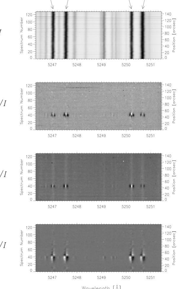
Figure 2.2: Sample spectrum of Stokes $I,Q,U$ and $V$.

In Fig.2.2 a sample Stokes $I,Q,U,V$ spectrum of a facular region near the solar limb is plotted. The 4 analyzed spectral lines are identified. These data were fully reduced following the tedious, but well-tested procedures described by Bernasconi (1997) [76].

2.2.2 Data set of March 2000

In order to improve the statistics and the $\mu$ coverage a second observing run was carried out in March 2000 with the Coud’e - Gregory Telescope in Locarno, Switzerland. This telescope is almost identical to the GCT on Tenerife and the parameters such as spectral resolution, noise level etc. are very similar to those of the 1995 observations.

The second generation, ZIMPOL II polarimeter (Gandorfer & Povel 1997, Povel 1998 [77, 78]) was employed for the polarization analysis and data recording. It simultaneously records three of the four Stokes parameters, either Stokes $I,Q,V$ or $I,U,V$ on a single CCD detector chip. Observations in these two modes were interlaced, such that alternate exposures record Stokes $I,Q,V$ and $I,U,V$, respectively. Exposures of the same Stokes parameters were then added together to reduce noise. Thus the final data set consists of all four Stokes parameters. The only differences with respect to the recordings made in 1995 are that the number of spatial pixels is reduced and that the noise level of Stokes $V$ in the newer data is a factor of $\sqrt{2}$ lower than of Stokes $Q$ and $U$, whereas Stokes $Q$, $U$ and $V$ had the same noise level in the earlier recordings. Due to the superior modulation scheme implemented in ZIMPOL II Stokes $Q$ and $U$ achieve a noise level of $10^{-3}I_{c}$ after roughly the same exposure time during the observations made in 2000 as during the earlier campaign.

These observations were carried out on the day of the equinox, at which time the two mirrors producing oblique reflections of the beam ahead of the modulator package are oriented such that their polarization cross-talk cancels out. Hence for these observations the instrumental cross-talk is essentially zero and no further treatment of the data for this effect is required.

The Sun was very active at the time of these observations with many active regions harboring sunspots and faculae present on the solar disc. Since active regions generally give larger amplitude Stokes signals we concentrated on observing them. A total of 7 exposures were made. The typical seeing during these observations was estimated to be $2-3^{\prime\prime}$, while the spatial pixel size was $1.13^{\prime\prime}$.

Figure 2.3: SOHO MDI intensity image from 22nd March 2000.

2.3 Data analysis

Each exposure gives us the line profiles of the 4 spectral lines in Stokes $I,Q,U$ and $V$ at a set of 94 (128 in the 1995 data) positions on the solar disc. Once the reduction and calibration procedure is completed we select from a given frame those spectra for further analysis for which the $S/N$ ratio for either Stokes $U$ or $V$ in at least one of the four spectral lines is above 12 in the 1995 data and above 15 in the 2000 data.

This criterion gave us a total of 4480 profiles from the four lines and were analysed further. The non-orthogonal wavelet-packets smoothing scheme of Fligge & Solanki (1998) [79] was employed to enhance the $S/N$ ratio by a factor of 1.5 - 2 without significantly affecting the profile shapes.

Then a set of parameters was determined of all Stokes profiles of all 4 spectral lines. Of these parameters only the signed amplitudes of the blue and red wings, $a_{\mbox{\footnotesize{b}}}$ and $a_{\mbox{\footnotesize{r}}}$ (i.e. of the blue and red Zeeman $\sigma$-component) are of relevance for the present study. In Fig. 2 we plot a Stokes $U$ and $V$ profile of the Fe I line at 5250.22Å. $a_{\mbox{\footnotesize{b,r}}}(V)$ and $a_{\mbox{\footnotesize{b,r}}}(U)$ are indicated in the figure. Using these we can form the symmetric and antisymmetric parts of the Stokes $V$ and $U$ profile amplitudes, $V_{\mbox{\footnotesize{s}}}=(a_{\mbox{\footnotesize{b}}}+a_{\mbox{\footnotesize{r}}})/2$, $V_{\mbox{\footnotesize{a}}}=(a_{\mbox{\footnotesize{b}}}-a_{\mbox{\footnotesize{r}}})/2$, $U_{\mbox{\footnotesize{s}}}=(a_{\mbox{\footnotesize{b}}}+a_{\mbox{\footnotesize{r}}})/2$ and $U_{\mbox{\footnotesize{a}}}=(a_{\mbox{\footnotesize{b}}}-a_{\mbox{\footnotesize{r}}})/2$, respectively, which enter Eqs. (2.1) and (2.2). In the following all $V$ and $U$ values and parameters are normalized to the continuum intensity, although this is often not explicitely mentioned.

Figure 2.4: Simultaneously measured profiles of Stokes $V$ and Stokes $U$ of the Fe I line at 5250.22Å.

2.3.1 Stokes asymmetry technique

A measure of the asymmetry of a Stokes profile is given by the ratio $\delta V=V_{\mbox{\footnotesize{s}}}/V_{\mbox{\footnotesize{a}}}$, respectively $\delta U=U_{\mbox{\footnotesize{a}}}/U_{\mbox{\footnotesize{s}}}$ (e.g. Solanki & Stenflo 1984 [64], Martínez Pillet et al. 1997 [68]) In Fig. 2.5 we plot these quantities vs. $|V_{\mbox{\footnotesize{a}}}|$ and $|U_{\mbox{\footnotesize{s}}}|$, respectively. Each point in these plots refers to a Stokes profile of the Fe I 5250.65Å line.

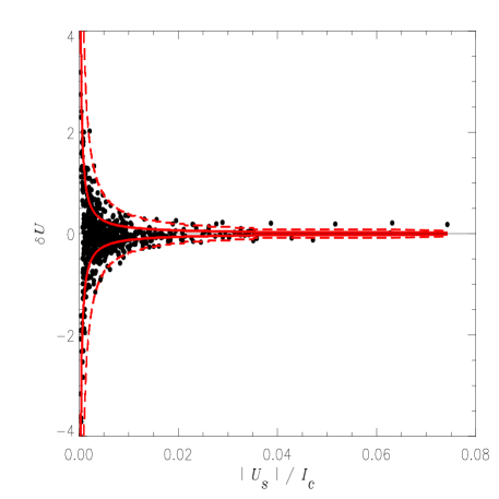
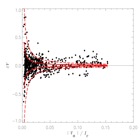
Figure 2.5: Measured amplitude asymmetries for Stokes $U$ and Stokes $V$.

Although our observations cover a range of $\mu$ values, Fig. 2.5 is very similar to corresponding figures based on data obtained near solar disc centre (Grossmann-Doert et al. 1996 [67], Martínez Pillet et al. 1997 [68]), where the influence of gravitational birefringence is expected to be negligible. For large amplitudes ($V_{\mbox{\footnotesize{a}}}$, $U_{\mbox{\footnotesize{s}}}$) the relative asymmetry ($V_{\mbox{\footnotesize{s}}}/V_{\mbox{\footnotesize{a}}}$,$U_{\mbox{\footnotesize{a}}}/U_{\mbox{\footnotesize{s}}}$) is small, while for weaker profiles it shows an increasingly large spread. For the weaker profiles this spread is mainly due to noise as can be judged from the solid and dashed curves in Fig. 2.5, which outline the $1\sigma$ and $3\sigma$ spread expected due to photon noise, respectively. The curves reveal that Stokes profiles with amplitudes ($V_{\mbox{\footnotesize{a}}}$, $U_{\mbox{\footnotesize{s}}}$) smaller than one percent of the continuums intensity are so strongly affected by noise that they are of little use for the present purpose. This leaves us with 1966 individual profiles for further analysis. In Fig.2.6 we plot a histogram of the number of these profiles as a function of $\mu$. The distribution is uneven, being determined by the position on the solar disc of magnetic features at the time of the observations.

Figure 2.6: Histogram of the number of profiles as a function of $\mu$.

The further analysis is made more complicated by the fact that a $V_{\mbox{\footnotesize{s}}}$ and a $U_{\mbox{\footnotesize{a}}}$ signal can be produced not just by gravitational birefringence, but also by radiative transfer processes acting in the dynamic solar atmosphere, as described in Sect. 3. To circumvent this problem we consider all profiles satisfying the criterion that $|V_{\mbox{\footnotesize{a}}}|$ or $|U_{\mbox{\footnotesize{s}}}|\geq 0.01$. For all these profiles $|\delta V_{\mbox{\footnotesize{obs}}}|<0.7$ and $|\delta U_{\mbox{\footnotesize{obs}}}|<0.6$. A similar picture is also obtained at the center of the solar disc. Hence one way to limit $\ell_{\odot}^{2}$ is to require $|\delta V_{\mbox{\footnotesize{src}}}|<1$ and $|\delta U_{\mbox{\footnotesize{src}}}|<1$ for all positions on the solar disc. This condition is strengthened by the fact that $|\delta V_{\mbox{\footnotesize{obs}}}|$ and $|\delta U_{\mbox{\footnotesize{obs}}}|$ decrease with decreasing $\mu$, (Stenflo et al. 1987 [81], Martínez Pillet et al. 1997 [68]), whereas gravitational birefringence increases towards the limb, so that one would expect exactly the opposite behaviour if gravitational birefringence had a significant effect on the Stokes $V$ or $U$ profiles.

In Fig.2.8 we plot the maximum $(U_{\mbox{\footnotesize{a,src}}}/U_{\mbox{\footnotesize{s,src}}})$ value predicted for each of the 4 spectral lines, based on all analysed data, vs. $\ell^{2}_{\odot}$. The horizontal line represents the value $\log(U_{\mbox{\footnotesize{a,src}}}/U_{\mbox{\footnotesize{s,src}}}=1)$, a limit above which this ratio is not observed at $\mu\approx 1$. Clearly, as $\ell^{2}_{\odot}$ increases $(U_{\mbox{\footnotesize{a,src}}}/U_{\mbox{\footnotesize{s,src}}})_{\mbox{\footnotesize{max}}}$ initially remains almost equal to $(U_{\mbox{\footnotesize{a,obs}}}/U_{\mbox{\footnotesize{s,obs}}})_{\mbox{\footnotesize{max}}}$, but begins to increase for $\ell^{2}_{\odot}\mathop{\raise 1.29167pt\hbox{$>$\kern-7.5pt\raise-4.73611pt\hbox{$\sim$}}}(50\,\mbox{km})^{2}$, becoming $\mathop{\raise 1.29167pt\hbox{$>$\kern-7.5pt\raise-4.73611pt\hbox{$\sim$}}}10$ at $\ell^{2}_{\odot}<(100\,\mbox{km})^{2}$ and finally oscillating randomly around $(U_{\mbox{\footnotesize{a,src}}}/U_{\mbox{\footnotesize{s,src}}})_{\mbox{\footnotesize{max}}}$ of 100 - 1000. All 4 spectral lines exhibit a similar behaviour, implying that the influence of noise is very small.The largest effect of gravitational birefringence is exhibited by the two most strongly Zeeman split lines, Cr I 5247.56Å, Fe I 5250.22 Å, which also produce the largest Stokes $V$ and $U$ signals, while the line with the smallest splitting, Fe I 5250.65 Å provides the weakest limit.

It is in principle sufficient to limit $\ell_{\odot}$ by requiring that none of the observed spectral lines has $(U_{\mbox{\footnotesize{a,src}}}/U_{\mbox{\footnotesize{s,src}}})>1$ within the range of allowed $\ell_{\odot}$ values. This gives $\ell^{2}_{\odot}<(57.1\,\mbox{km})^{2}$. A limit obtained similarly from Stokes $V$ is both larger $\ell^{2}_{\odot}<(80.3\,\mbox{km})^{2}$ and less reliable, since we cannot completely rule out $V_{\mbox{\footnotesize{s,src}}}/V_{\mbox{\footnotesize{a,src}}}>1$ to be present, although we expect such profiles to be very rare, among large amplitude profiles.

Fig.2.8 shows the analogous plot for metric affine theories. As in the above case for Moffat’s NGT it can be seen that the strongest limit for gravity-induced birefringence is exhibited in the Cr I 5247.56Å and Fe I 5250.22Å line. We get $k^{2}<(1.1\,\mbox{km})^{2}$ from Cr I 5247.56Å and $k^{2}<(0.9\,\mbox{km})^{2}$ from Fe I 5250.22Å.

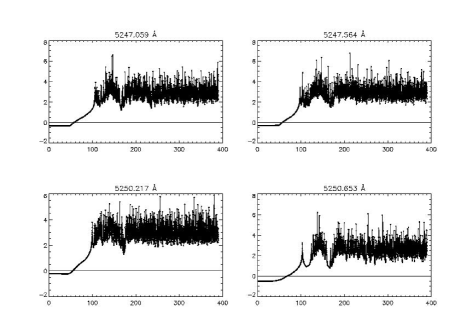
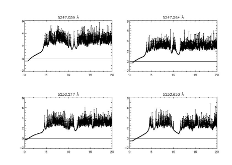
Figure 2.7: Maximum of $(U_{\mbox{\footnotesize{a,src}}}/U_{\mbox{\footnotesize{s,src}}})$, on a logarithmic scale, values for all 4 spectral lines vs. $\ell^{2}_{\odot}$.

Figure 2.8: Maximum of $(U_{\mbox{\footnotesize{a,src}}}/U_{\mbox{\footnotesize{s,src}}})$, on a logarithmic scale, values for all 4 spectral lines vs. the metric affine parameter $k$.

An alternative test is to determine the fraction of profiles with $(U_{\mbox{\footnotesize{a,src}}}/U_{\mbox{\footnotesize{s,src}}})>1$ (Fig.2.9) Fig.2.9 reveals that initially no $U$ profile satisfies the criterion, above $\ell^{2}_{\odot}=(57.5\,\mbox{km})^{2}$ 1.5 % of the profiles does. This number keeps increasing with $\ell_{\odot}$, before finally oscillating around 70% at large $\ell_{\odot}$. Thus 10% of all data points have $(U_{\mbox{\footnotesize{a,src}}}/U_{\mbox{\footnotesize{s,src}}})>1$ for $\ell^{2}_{\odot}=(74.0\,\mbox{km})^{2}$, 20% for $\ell^{2}_{\odot}=(79.4\,\mbox{km})^{2}$. We are not aware of any solar observations of Stokes $U$ with $\delta U>1$ for which instrumental cross-talk is negligible (see Sánchez Almeida & Lites 1992 [70], Skumanich et al. 1990 [82]). $\ell_{\odot}^{2}<(80\mbox{km})^{2}$ is thus a very conservative upper limit.

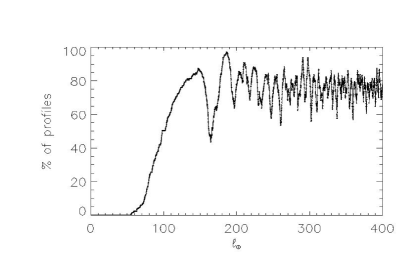
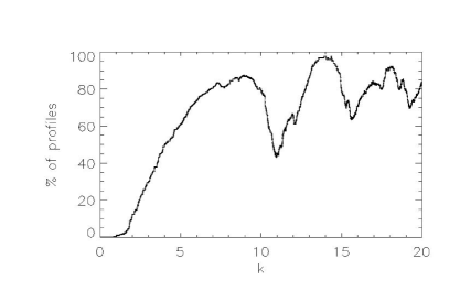
Figure 2.9: Fraction of profiles with $(U_{\mbox{\footnotesize{a,src}}}/U_{\mbox{\footnotesize{s,src}}})>1$ for NGT (top) and MAG (bottom).

The lower picture shows the analogous plot for metric affine theories. Also, initially no profile satisfies the criterion, above $k^{2}=(1.33\,\mbox{km})^{2}$ 1.7 % of the profiles does. This number keeps increasing with $\ell_{\odot}$, before finally oscillating around 70% at large $k$. Thus 10% of all data points have $(U_{\mbox{\footnotesize{a,src}}}/U_{\mbox{\footnotesize{s,src}}})>1$ for $k^{2}=(1.95\,\mbox{km})^{2}$, 20% for $k^{2}=(2.43\,\mbox{km})^{2}$. $k^{2}<(2.5\mbox{km})^{2}$ is thus a very conservative upper limit.

2.3.2 Profile difference analysis

We now apply the technique outlined in Sect. 2.1.2 to our data. Due to the limited number of profiles and their irregular distribution over $\mu$ (see Sect. 2.3.1) any limit on gravitational birefringence will be less tight than what is achievable with ideal data presented in Sect. 2.1.2. In order to be able to compare the present results with literature values we first set limits on the $\ell_{\odot}$-parameter in Moffat s NGT, since earlier work has concentrated on constraining this theory.

In Fig.2.10 we plot

$$\frac{|<|V_{\mbox{\footnotesize{obs}}}|>-<|U_{\mbox{\footnotesize{obs}}}|>|}{<|V_{\mbox{\footnotesize{obs}}}|>+<|U_{\mbox{\footnotesize{obs}}}|>}\quad\mbox{vs.}\quad\ell_{\odot},$$ (2.3)

for different initial phase differences $\Delta\Phi$ between the orthogonal modes of line Fe I 5250.65Å. The averaging has been done over the $\mu$ values at which observations are available.

Figure 2.10: Plot of the observable (Stokes $V$, Stokes $U$) mixture for initial phase differences of $0\pi$, $0.1\pi$, $0.25\pi$ and $0.4\pi$. Note that $\Delta\Phi$ values bigger than $0.5\pi$ give cyclic results.

This line is chosen, since it gives the tightest limits on $\ell_{\odot}^{2}$. The thick horizontal line represents the value obtained from observations. Obviously above $\ell_{\odot}^{2}=(178\,\mbox{km})^{2}$ the curve obtained from theory always lies below the observed value, hence ruling out such $\ell_{\odot}^{2}$ values. Note that it is sufficient to test for $\ell^{2}_{\odot}<(305\,\mbox{km})^{2}$, since this upper limit has been set using independent data and another technique by Solanki & Haugan (1996) [63].

Similarly we can also set a limit on the coupling constant $k$ of the metric affine theories. Using this technique we obtain $k^{2}<(0.69\,\mbox{km})^{2}$ measured in line Fe I 5250.65Å.

2.3.3 Brief history of constraints on $\ell_{\odot}^{2}$

Up to this point we have presented our results with respect to sharp constraints on the coupling constants $\ell_{\odot}^{2}$ and $k^{2}$. In order to get an estimate of the quality of these results compared to previous upper limits we will present here a brief overview on the history of constraints on $\ell_{\odot}^{2}$ achieved with a variety of different techniques.

The first upper bound on the value of the NGT charge $\ell^{2}_{\odot}$ was given by Moffat himself in 1982 [39]. Based on a new determination of the quadrupole moment of the sun he concluded that this result would lead to a deviation of 1.6% from Einstein’s prediction for the precession of the perihelion of Mercury. Moffat claimed that NGT could fit the measured precession with the new quadrupole moment by using a value of $\ell_{\odot}=3.1\cdot 10^{3}\,\mbox{km}$ close to the upper bound of $\ell_{\odot}\leq 2.9\cdot 10^{3}\,\mbox{km}$ obtained in 1982 by using an average value on the available Mercury data.

The next significant improvement was made by Gabriel et al. in 1991 [22]. By using for the first time the NGT prediction of gravity-induced birefringence they presented a quantitative prediction for the phase difference between the orthogonal modes. Consequently, birefringence leads to a depolarization of the Zeeman components of spectral lines emitted from extended, magnetically active regions on the sun. Since the solar-physics data which were available at that time limited the extend of such depolarization, they could only conclude that the Sun’s antisymmetric charge must be less than $(535\,\mbox{km})^{2}$.

This result was based on extremely conservative assumptions regarding the polarization of light emitted by the observed solar feature and an inapplicable requirement regarding the determination of the magnetic filling factor, which is defined as the fraction of the aperture covered by magnetic field. In 1995 Solanki and Haugan [63] improved the limit on $\ell^{2}_{\odot}$ by using more realistic values of the parameters that characterize the solar polarization source and a refined analysis procedure which yielded an upper bound of $\ell^{2}_{\odot}<(305\,\mbox{km})^{2}$.

The current work represents the state of the art with respect to upper limits on gravitational birefringence induced by the nonsymmetric field of the sun. Since the physical consequences of the nonmetric NGT description relevant for our purpose are proportional to $\ell^{4}_{\odot}$ this new constraint on the Sun’s NGT charge is three orders of magnitude smaller than the previous limit by Solanki and Haugan and 7 orders of magnitude smaller than the value favoured initially by Moffat. This gives a further significant restriction to the viability of NGT.

2.4 Possible tests using the Solar Probe spacecraft

       

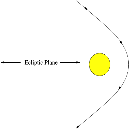
Figure 2.11: Left figure: Sketch of the Solar Probe trajectory near the sun as seen from Earth. Right figures: Expected phase shifts for a signal emitted at $3R_{\odot}$ from the sun. Top: Optical wavelength. Bottom: Soft X-ray.

The possibility of setting strong limits on gravitational birefringence with the tests which we have outlined so far suffered from the major drawback that they all depend strongly on our knowledge of solar magnetic features. For example we have assumed that none of the observed spectral lines has $(U_{\mbox{\footnotesize{a,src}}}/U_{\mbox{\footnotesize{s,src}}})>1$ which is also based on current observations with a certain spatial resolution. At the moment nobody can say if this statement will hold if the instrumental resolution could be highly increased in the future, although simulations of solar magnetoconvection suggest that $U_{\mbox{\footnotesize{a,src}}}<U_{\mbox{\footnotesize{s,src}}}$ remains valid even if the resolution is improved by an order of magnitude.

Taking this into account, it is obvious that drastic improvements of our limits for $\ell^{2}_{\odot}$ could be achieved by using an artificial source for the polarized radiation with well defined properties, placed in close vicinity to the sun. Such a source could possibly be provided by the Solar Probe spacecraft [83], which is part of NASA’s mid-term plans. Designed mainly as a mission to explore the Sun’s Corona, its trajectory (sketched in Fig.a) lies in a plane perpendicular to the ecliptic with a target perihelion distance at 3-4 solar radii. This close perihelion could provide a unique opportunity to look for gravitational birefringence if it is possible to receive a well defined polarized signal from an instrument onboard the spacecraft when it passes near the solar limb.

To see, if we could expect a reasonable gravitational effect in the signal, we simply have to take the case $\mu=0$ in the phase shift formula (1.57) and replace the solar radius $R_{\odot}$ with $(R_{p}+1)\cdot R_{\odot}$ where $R_{p}$ is the perihelion distance of the spacecraft in units of the solar radius. This leads to

$$\big{.}\Delta\Phi\;\big{|}_{\mu=0}=\frac{3\,\ell^{4}_{\odot}\,\pi^{2}}{16\,\lambda\,((R_{p}+1)\cdot R_{\odot})^{3}}$$ (2.4)

Of course this result depends strongly on the wavelength of the signal. The shorter the wavelength the bigger is the possible phase shift that we could expect. This is illustrated in Fig.(2.11b), which shows the phase difference in units of $\pi$ for a range of $\ell_{\odot}$ values with $R_{p}=3$. Optical wavelength is used in the upper diagram and X-ray in the lower. One can see that for optical wavelength a gravitational effect on the polarization of the signal would be extremely difficult to observe under realistic conditions with a certain noise level. Whereas for wavelengths of the order $10^{-10}$m, we could expect a reasonable transformation of linear to circular polarization and vice versa for $\ell^{2}_{\odot}$ values which are clearly below our current upper limit. However, at the moment it is out of reach from the technological point of view, to place a source of polarized X-rays in the near vicinity of the sun. Nevertheless it is worth to keep this promising possibility for very precise tests of the Einstein equivalence principle in mind.

2.4.1 Alternative Spacecraft Trajectories

Figure 2.12: Expected phase shifts for a signal emitted at $3R_{\odot}$ from the sun when the spacecraft passes in front of the solar disc on an alternative trajectory. The wavelengths are the same as in Fig.2.11

Interestingly the planned spacecraft trajectory is also a very suitable one with respect to possible tests of gravity-induced birefringence. This is due to the fact that when the spacecraft reaches its perihelion position the phase shift is maximized by the mimimal distance to the sun, i.e. highest gravitational potential, and also by the maximum distance that the signal could travel through the gravitational field of the sun.

If the craft reaches on a different trajectory its closest position to the sun which is also closer towards earth this would mean a shorter distance for the signal to travel and, hence, a smaller total phase shift. This is shown for a spacecraft passing in front of the visible solar disc at distance $R$ to the sun. The phase shift of a signal with wavelength $\lambda$ emitted at this position is given by

$$\big{.}\Delta\Phi\;\big{|}_{\atop{\mu=0\atop R\rightarrow\infty}}=\frac{\pi\l^{4}_{\odot}}{\lambda}\left(\frac{3\pi}{16R_{0}^{3}}-\frac{R}{2}\left(\frac{1}{2(R_{0}^{2}+R^{2})^{2}}+\frac{3}{4R_{0}^{2}(R_{0}^{2}+R^{2})}\right)-\frac{3}{8R_{0}^{3}}\arctan\frac{R}{R_{0}}\right)\quad.$$ (2.5)

The detailed calculation is given in Appendix B. Fig.2.12 shows the result for the same wavelength as in Fig.2.11 and $\mu=0$. The cumulative phase shift for the alternative trajectory is smaller by a factor of 15 although the distance to the sun is the same in both cases. The crucial point is that in the first case the signal covers a bigger distance within that region of the gravitational field where it is strong enough to induce a reasonable phase shift. This relevant distance has an extend of approximately 5-6 solar radii. A different trajectory where the spacecraft passes the visible limb behind the sun as seen from earth would give no improvement since the phase shift which accumulates from behind the sun up to a position above the poles has an opposite sign compared to the phase shift of a signal which is emitted above the pole, propagating towards earth. This can be seen from equation (B.8) in Appendix B which gives the phase shift for a signal running from the surface up to a distant point $R$. If the signal runs in the opposite direction we have to switch the integration limits which gives a negative sign for the phase shift.

2.5 Discussion and Conclusions

Using two techniques (the Stokes asymmetry technique and the new profile difference technique) we have improved previous limits on $\ell^{2}_{\odot}$ given by Solanki & Haugan (1996) [63] by nearly one order of magnitude. It will be difficult to set much tighter limits on gravitational birefringence than those found here using solar data in the visible spectral range. To obtain a significant improvement on the basis of solar data one would need to observe at shorter wavelengths. The line at the shortest wavelength that is strong enough to provide a hope of detecting Stokes $U$ and $V$ at sufficient $S/N$ is Ly$\alpha$ at 1216Å. The maximum gain that one could expect relative to the current analysis is a factor of

$$\frac{\lambda_{\mbox{\footnotesize{visible}}}}{\lambda_{\mbox{\footnotesize{Ly}}\alpha}}=\frac{5250}{1216}=4.32\quad.$$ (2.6)

Although the idea of a possible utilization of future space missions for enhanced new tests is very appealing because of its high potential for further improvements of the current limits on $\ell^{2}_{\odot}$ and $k^{2}$, the technological realization of such an experiment is currently out of reach. For setting stronger limits on gravitational birefringence or, if birefringence really has a physical relevance, for having the chance of a direct detection of this effect it is therefore more promising to proceed the investigations with more compact astrophysical objects. This will be the content of the following chapters.

Chapter 3 Magnetic White Dwarfs

The conjecture that gravity-induced birefringence is most distinctive for high gravitational potentials suggests itself from the structure of the phase shift formulas in NGT and MAG. For this reason the next logical step in this work is to continue the analysis with suitable, compact objects like magnetic white dwarfs. These stars provide a versatile tool for testing predictions of nonmetric theories of gravity because of their Megagauss magnetic fields and high surface gravity. Currently 65 or $\sim 5$% of all known white dwarfs are classified as isolated magnetic stars with field strengths in the range $3\times 10^{4}-10^{9}$G with the field strength distribution peaking at $1.6\times 10^{7}$G [87].

However, within this small class only a fraction of stars is of interest for our purpose. In addition to wavelength resolved polarimetric data we also need information about the mass and the radius of an object as well as measurements of the magnetic field structure to set strong limits on gravitational birefringence. With these restrictions we are left with just four magnetic white dwarfs which display high levels of circular polarization between 8 and 22 percent: Grw $+70^{\circ}8247$, REJ0317-853, PG2329+267 and 40 Eridani B. The degree of circularly polarized light of wavelength $\lambda$, $(V/F)_{\mbox{\footnotesize{obs}}}$, reaching the observer from any of these stars is to first order simply a function of the strength of the local longitudinal magnetic field [85] and the coupling constant $k^{2}$. Since gravitation theories based on a metric-affine geometry of space-time predict a depolarization of light emitted from extended astrophysical sources we have looked for the largest $k^{2}$ that predicts values of $(V/F)_{\mbox{\footnotesize{obs}}}$ larger than or equal to that observed. This sets an upper limit on $k$. In the case of Grw $+70^{\circ}8247$ such a limit was already set by Solanki et al.[86] based on NGT predictions. We redo the analysis using both an improved model of the magnetic field distribution of the star, as well as the predictions of metric affine theory, which had not been predicted earlier.

However, we encounter a self-consistency problem since the relevant source properties like masses, inclination angles, etc. we use have been determined with models which, of course, neglect the possible influence of birefringence and, so, need not be valid. We circumvent this problem by assuming worst-case properties of the source that minimize depolarization caused by gravity-induced birefringence.

3.1 Polarization Modelling Technique

The search for a possible influence of gravity-induced birefringence on astronomical signals, i.e. the modelling technique which is used to set strong upper limits, depends of course heavily on the amount of appropiate information that we can gain on the source of polarized radiation. This becomes decisively clear in the transition from the techniques which we have used to evaluate the solar observations of the last chapter to the magnetic white dwarfs. Here, a crucial point is basically played by the spatial resolution of the observations, since the individual calculation of the phase shift $\Delta\Phi$ as a function of $\mu$ for a given light source requires, at least theoretically, an infinite resolution of the source.

So, due to the finite spatial resolution of observations, the effect the phase shift has on a light ray depends on whether one observes a pointlike source, e.g. small sunspots, or an extended source like white dwarf magnetospheres. In the case of a pointlike source, all light received from it suffers the same phase shift $\Delta\Phi(\mu_{p})$. Introducing Stokes parameters to describe polarized light, with Stokes $Q$ defined to represent the difference between linear polarization parallel and perpendicular to the part of the stellar limb closest to the source, one therefore finds a crosstalk between Stokes $U$ and Stokes $V$. This crosstalk is such that although the observed values $U_{\mbox{\footnotesize{obs}}}$ and $V_{\mbox{\footnotesize{obs}}}$ differ from the values emitted by the source, $U_{\mbox{\footnotesize{src}}}$ and $V_{\mbox{\footnotesize{src}}}$, the composite degrees of polarization remains equal: $(U_{\mbox{\footnotesize{obs}}}^{2}+V_{\mbox{\footnotesize{obs}}}^{2})^{1/2}=(U_{\mbox{\footnotesize{src}}}^{2}+V_{\mbox{\footnotesize{src}}}^{2})^{1/2}$. If an extended source covering a range of $\mu$ values is observed then light emitted from different points suffers different phase shifts and, so, adds up to an incoherent superposition. Summing over the different contributions, using the additive properties of Stokes parameters yields a reduction of the observed polarization relative to the light emitted from the source: $(U_{\mbox{\footnotesize{obs}}}^{2}+V_{\mbox{\footnotesize{obs}}}^{2})^{1/2}<(U_{\mbox{\footnotesize{src}}}^{2}+V_{\mbox{\footnotesize{src}}}^{2})^{1/2}$. Since the stellar sources of polarization we consider in this chapter are spatially extended, any observed (nonzero) degree of polarization provides a limit on the strength of gravity-induced birefringence that the star’s gravitational field could induce.

It is generally agreed that the polarized radiation from white dwarfs is produced at the stellar surface as a result of the presence of Megagauss dipolar magnetic fields [98, 99]. To first approximation the flux of net circularly polarized light at wavelength $\lambda$ emitted toward the observer from the surface is directly proportional to the strength of the line of sight component of the magnetic field at the stellar surface. Therefore, this net flux can be written as

$$V_{\lambda,\mbox{\footnotesize{src}}}=2\pi\int_{0}^{1}I_{\lambda}(\mu)\cdot w(\mu)\mu\,d\mu\quad,$$ (3.1)

where $I(\mu)$ is the intensity at wavelength $\lambda$. The weightfunction $w(\mu)$ describes the strength of the vertical magnetic field component at position $\mu$. Since our analysis encompasses different white dwarfs with different types of dipole field geometries, $w(\mu)$ is calculated using an oblique dipolar rotator model which is introduced in the next section.

To define a degree of circular polarization, we have to divide (3.1) by the total stellar flux emitted to the observer at wavelength $\lambda$

$$F_{\lambda}=2\pi\int_{0}^{1}I_{\lambda}(\mu)\mu\,d\mu\quad.$$ (3.2)

The function $I_{\lambda}(\mu)$ also describes the limb darkening of the star. Since the surface of a white dwarf cannot be resolved the limb darkening cannot be measured directly. Because the broadband spectrum of Grw +70^∘8247 is well represented by blackbody radiation [100] and radiative equilibrium models [133, 101] it is reasonable to assume a simple law like the one describing the directly observed solar limb darkening. For this, we have chosen to use [103]

$$\frac{I_{\lambda}(\mu)}{I_{\lambda}(\mu=1)}=1+(\mu-1)g+(\mu^{2}-1)h\quad,$$ (3.3)

with

$$0\leq g+h\leq 1$$

for Grw +70^∘8247. Since this kind of a linear interpolation is of a very general form we have taken the limb darkening model of Grw +70^∘8247 as a prototype for the white dwarfs within our sample.

In practise, we have evaluated the degree of circular polarization $(V_{\lambda,\mbox{\footnotesize{src}}}/F_{\lambda})$ numerically for increasing values of $k_{\star}$ and, in the case of Grw +70^∘8247, of $l_{\star}$. In contrast to the earlier work of Solanki, Haugan and Mann [86] (1999) we assume that the light emitted by the source is polarized proportional to ${\bf B}$, i.e. to $w(\mu)$.

3.2 Oblique dipolar rotator model

The model we use was already described by Stift in 1975 [104] from whom we adopted most of our notations.

Starting with the observer’s system where the z-axis is defined by the line-of-sight, a surface point on the visible hemisphere of the star is given by ${\bf z}$. This vector is transformed into the rotation system of the star by the matrix

$$S_{i}=\left(\begin{array}[]{rrr}1&0&0\\ 0&\cos i&\sin i\\ 0&-\sin i&\cos i\end{array}\right)\quad,$$ (3.4)

which is followed by a rotation around the rotational z-axis

$$S_{\phi}=\left(\begin{array}[]{rrr}\cos\phi&\sin\phi&0\\ -\sin\phi&\cos\phi&0\\ 0&0&1\end{array}\right)\quad.$$ (3.5)

The position of the dipole system relative to the rotational system is uniquely described by the three Eulerian angles, e.g. by

$$S=S_{\xi}S_{\zeta}S_{\chi}$$ (3.6)

where $S_{\xi}$ and $S_{\chi}$ are generating rotations around the x-axis and $S_{\zeta}$ around the z-axis. Since the only measurable quantity in observations is the resulting tilt angle $\beta$ between the dipole and rotation axis, the effect of the three Eulerian rotations can be summarized without loss of generality by a rotation with $\beta$ around the x-axis.

Given the offset coordinates of the dipole in the rotation system by ${\bf x}$, we obtain the coordinates of the surface point ${\bf z}$ relative to the dipole system by

$${\bf r}=S_{\beta}(S_{\phi}S_{i}{\bf z}-{\bf x})\quad,$$ (3.7)

so that the field strength in the dipole system is given by

$${\bf B}_{dp}=-\nabla({\bf m}\cdot{\bf r}/r^{3})\quad.$$ (3.8)

From this we get the field strength in the observer’s system through

$${\bf B}_{obs}=S_{i}^{T}S_{\phi}^{T}S_{\beta}^{T}{\bf B}_{dp}$$ (3.9)

where $S_{i}^{T},\,S_{\phi}^{T},\,S_{\beta}^{T}$ are the transpose matrices of $S_{i},\,S_{\phi},\,S_{\beta}$. The longitudinal field component in the observer’s system is then of course the ${\bf B}_{obs,z}$ component of (3.9).

The effective field ${\bf B}_{e}$ for the visible hemisphere is then given by

$${\bf B}_{e}=\int\int{\bf B}_{z}I\,dA\bigg{/}\int\int I\,dA\quad.$$ (3.10)

${\bf B}_{z}$ denotes the line-of-sight component of ${\bf B}_{obs}$, while the limb darkening is described, as above, by the empirical function $I$.

Figure 3.1: Geometrical representation of the dipole- relative to the rotation system of the star with offsets. The rotation axis is inclined to the observer by an angle $i$. In general, the offset dipole is tilted against the rotation axis as described in Fig.3.2.

3.3 Grw +70^∘8247

Within the class of magnetic white dwarfs, Grw +70^∘8247 has played the role of a ”Rosetta stone” in the analysis and interpretation of their spectra. Although the first measurement of circular and linear polarization in the spectrum of a white dwarf [88] gave a strong indication for a magnetic field, the presence of broad absorption features in its blue spectrum remained unexplained until the 1980s. A solution of this puzzle was only given after detailed calculations of hydrogen energy levels at field strengths $B>100$ MG [89, 90, 91, 92] so that, as a result, all spectral features could consistently be explained in terms of stationary lines, i.e. lines whose wavelengths vary only slowly with the field strength, of atomic hydrogen in a centered dipolar magnetic field with a polar field strength of $\sim 320$ MG and a viewing angle (angle between the line of sight and the magnetic axis) $i=0^{\circ}-30^{\circ}$ [133, 93, 94].

In this way it was possible to determine the physical parameters of the stellar atmosphere and of the magnetic field from a best fit of synthetic to observed spectra. The observations can be best explained by an effective temperature of 14,000 K [133, 100] which implies a radius of 0.0076 $R_{\odot}$ (determined from photometry and parallax distance measurements), where $R_{\odot}$ is the solar radius, and a mass of about 1.0 $M_{\odot}$, where $M_{\odot}$ is the solar mass [102]. Since the characteristics of the polarization curve have remained invariant for almost $\sim 25$ yr now [87] we can infer a very long rotation period of much more than 25 years. This slow rotation is fitted into the obique rotator model by setting $\beta=0$, implying a dipole aligned with the rotation axis. Thus at a given point in the observer system with polar coordinates $(r,\theta,\phi)$, the Cartesian field components in the case $i=0^{\circ}$ are simply given by

$$B_{x} = 3B_{d}\sin\theta\cos\theta\cos\phi/2r^{3}\quad,$$ (3.11)

$$B_{y} = 3B_{d}\sin\theta\cos\theta\sin\phi/2r^{3}\quad,$$ (3.12)

$$B_{z} = B_{d}(3\cos^{2}\theta-1)/2r^{3}\quad,$$ (3.13)

where $B_{d}$ denotes the surface polar field strength for the case of a centered dipole. In our case, the z-axis is also the line of sight. Since we focus on measurements of circular polarization, only the longitudinal Zeeman-Effect is relevant for our purpose.

Polarization measurements of Grw +70^∘8247 yielded a level of $-6\pm 0.25$% in the visible spectrum at 449 nm [95, 96, 97]. Since the constraints on $k_{\star}^{2}$ and $l_{\star}^{2}$ are stronger for larger observed degrees of polarization and shorter wavelengths we make use of Hubble Space Telescope spectropolarimetry in the ultraviolet, which revealed high levels of circular (12%) and linear (20%) polarization. This was measured between 130 and 140 nm and is related to the absorption feature at 134.7 nm [97]. To be conservative, we assume a large absolute error of 1% on these measurements, and use a degree of circular polarization of 11% at 134.7 nm.

In 1999 Solanki, Haugan and Mann [86] have used the NGT prediction to set strong upper limits on $l^{2}_{\star}$ of the magnetic white dwarf Grw +70^∘8247 with a very simple model of the magnetic field distribution. Although it became clear in the meantime that NGT suffers from technical problems that render it mathematically inconsistent, we also carry out the analysis based on Eq.(1.57) for Grw +70^∘8247, in order to have a quantitative comparison between the old, unrealistically simple and the improved model incorporating an oblique rotator of the magnetic field.

The results of our analysis can be seen in Fig.(3.4) and Fig.(3.4) Our search for the largest values of $k_{\star}$ and $l_{\star}$ compatible with the observed degree of cicular polarization at 134.7 nm yields the constraints $k^{2}_{\star}\leq(0.074\,\mbox{km})^{2}$ and $l^{2}_{\star}\leq(4.1\,\mbox{km})^{2}$ for a viewing angle $i=0^{\circ}$. This limit on $l^{2}_{\star}$ is to be compared with the former limit $l^{2}_{\star}\leq(4.9\,\mbox{km})^{2}$. These results were obtained for limb darkening coefficients $(g,h)=(0,1)$, which provide the most conservative constraints. Neglecting limb darkening yields $k^{2}_{\star}\leq(0.06\,\mbox{km})^{2}$ and $l^{2}_{\star}\leq(3.7\,\mbox{km})^{2}$ compared with the old constraint $l^{2}_{\star}\leq(4.6\,\mbox{km})^{2}$. For other values of the $(g,h)$ pair the constraint on $k_{\star}$ and $l_{\star}$ falls between these extremes.

For increasing viewing angle $i$ to the dipole axis the maximum degree of circular polarization decreases, due to the dipole field geometry. From this it follows that constraints on $k_{\star}$ become stronger for larger $i$, although the dependence turns out to be weak. E.g. for $i=30^{\circ}$, we obtain the tiny improvement $k^{2}_{\star}\leq(0.072\,\mbox{km})^{2}$ with limb darkening and $k^{2}_{\star}\leq(0.058\,\mbox{km})^{2}$ without limb darkening. Hence the most conservative estimate is for $i=0$, which we adopt.

         

Figure 3.2: Left figure: Projection of the conelike movement of the magnetic pole during the rotational period onto the celestial plane for $\beta\neq 0$. Right figure: Relative orientation of the line-of-sight to the dipole axis and the rotational axis. Adopted from Burleigh, Jordan and Schweizer [107].

   

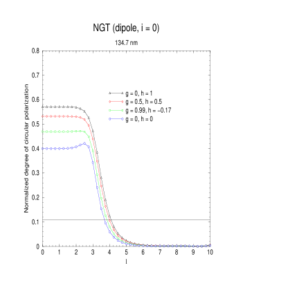
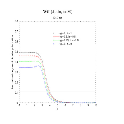
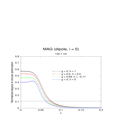
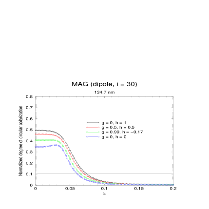
Figure 3.3: Observed degree of circularly polarized light for increasing values of $\ell_{\star}$ from NGT, normalized to full intensity $I=1$. Left figure: Dipole inclination $i=0^{\circ}$. Right figure: Dipole inclination $i=30^{\circ}$. The different curves are for different limb darkening parameters. The horizontal line represents the observed value of 11%.

   

Figure 3.4: Observed degree of circularly polarized light for increasing values of $k_{\star}$ from metric-affine gravity, normalized to full intensity $I=1$. Left figure: Dipole inclination $i=0^{\circ}$. Right figure: Dipole inclination $i=30^{\circ}$. The different curves are for different limb darkening parameters. The horizontal line represents the observed value of 11%.

3.4 RE J0317-853

3.4.1 Introduction

RE J0317-853 is certainly a highly unusual object which sets several records within the class of isolated magnetic white dwarfs. Discovered in 1995 as an extreme-ultraviolet source during the ROSAT Wide Field Camera (WFC) all-sky survey by Barstow et al. [108] (hereafter B95) the analysis of B95 revealed an unusual hot white dwarf with an effective temperature of $\approx 50000$ K and an exceptionally intense dipolar magnetic field of $\approx 340$ MG. B95 also reported nearly identical photometric and polarimetric variations of 725.4 s. Since the most plausible explanation is that these modulations are due to the rotation of the star, this would lead to the fastest rotation period ever measured so far among the isolated magnetic white dwarfs which have typical periods of several hours. Finally, the close proximity of the ordinary, DA white dwarf LB09802, separated by only 16” allowed B95 identify RE J0317-853 as a member of a double degenerate pair, which then enabled them to estimate the mass of RE J0317-853 at $1.35\,M_{\odot}$, close to the Chandrasekhar limit, which makes it the so far most massive known isolated white dwarf with a corresponding radius of only $0.0035\,R_{\odot}$. They found that their data are best matched by a dipole model with a negative offset along the dipole axis of 20% viewed at an angle of $60^{\circ}$. Polarization measurements were not reported by B95.

Ferrario et al. (hereafter F97) modelled phase-averaged spectropolarimetric data of RE J0317-853 in 1997 and obtained a dipole model with a polar field strength of $B_{d}=450$ MG and a negative offset of 35% of the stellar radius along the dipole axis. Their best fits were derived for mean viewing angles to the dipole axis of $30^{\circ}-60^{\circ}$. Furthermore, they reported variations in the wavelength-averaged circular polarization data at a period of $725\pm 10$ s which confirmed the results from B95. More important for our work is that F97 also found circular polarization in the continuum up to a maximum of 8% in the wavelength range from 5600 Å - 5800 Å. To be conservative, we adopted for our purpose the maximum value of 5800 Å and as for the B95 data the maximum limb darkening coefficients $g=0,\,h=1$.

The so far most detailed investigation regarding the magnetic field geometry of RE J0317-853 was published by Burleigh, Jordan and Schweizer in 1999 [107]. Using phase-resolved, far-UV HST Faint Object Spectrograph spectra they obtained the best fit for a dipole with $B_{d}=363$ MG and additional offsets perpendicular to the $z$-axis: $x_{\mbox{\footnotesize{off}}}=0.057,\,y_{\mbox{\footnotesize{off}}}=-0.04$ and $z_{\mbox{\footnotesize{off}}}=-0.22$. In this model the rotation axis is viewed at an angle of $i=50^{\circ}$ to the observer while the relative angle between rotation and dipole axis was found to be $\beta=42^{\circ}$, leading to visible surface field strengths between 140 and 730 MG. In addition they reported the limb darkening coefficients $g=0.3$ and $h=0$. In 1999 Jordan and Burleigh (hereafter JB99 [110]) reported a peak level of circular polarization at $22$% integrated over the wavelength range between 3400 Å and 7000 Å measured in spectropolarimetric data taken with the AAT (Anglo-Australian Telescope). This is up to now the highest level of circular polarization ever recorded for a magnetic white dwarf. Although it seems very likely from the data in JB99 that the real wavelength range in which the high level of circular polarization was measured is between 5600 Å and 5800 Å this conjecture was so far not confirmed by the authors.

3.4.2 Birefringence analysis

Figure 3.5: Successive rotational phases of RE J0317-853 in steps of $0.25\pi$, beginning with $\phi=0.25\pi$ (top left) to $\phi=2\pi$ (bottom right). The dashed line markes the stellar equator whereas the solid line shows the projection of the magnetic equator on the stellar surface. The cross marks the position of the rotation axis and the dot the position of the magnetic pole.

Due to its small radius and high degree of circular polarization, RE J0317-853 is a very suitably object concerning limits on gravitational birefringence. Unfortunately the wavelength range in which the polarization was measured by F97 as well as by JB99 lies in the optical regime and additionaly is up to now not very well isolated in the case of the 22% measurement of JB99 [110]. So, in order to get here conservative and reliable upper limits on gravitational birefringence we use 7000Å which marks the upper end of the measured spectral range. For comparison we also present our estimates in the case of 5800 Å as the upper wavelength end.

For our analysis of the JB99 data we also need information about the magnetic field geometry at that rotation phase, when the highest degree of polarization is emitted towards the observer. Since the highest degree is obtained for the highest average longitudinal magnetic field strength over the visible hemisphere we have plotted in Fig.(3.5) successive rotational phases of RE J0317-853 in steps of $0.25\pi$ based on the reported offset values $x_{\mbox{\footnotesize{off}}}=0.057,\,y_{\mbox{\footnotesize{off}}}=-0.04,\,z_{\mbox{\footnotesize{off}}}=-0.22$, limb darkening coefficients $g=0.3,\,h=0$ from (3.3) and the angles $i=50^{\circ}$ and $\beta=42^{\circ}$ by Burleigh, Jordan and Schweizer [107]. The longitudinal field strength on the surface is colorcoded whereby the blue color denotes positive and the red color negative polarity. It can be seen, that in phase $\phi=0.25\pi$ the different polarities nearly cancel each other so that the disk averaged field strength is approximately zero. During the progression of the rotation the average field strength increases up to $\phi=\pi$ and then subsequently decreases. This is also quantitatively shown in Fig.(3.6).

Figure 3.6: Integrated longitudinal $({\bf B}_{z})$ magnetic field strength of the visible hemisphere for successive rotational phases of RE J0317-853.

So, by using the oblique rotator model, described in Sec. 3.2 we obtain an upper limit of $k^{2}_{\star}\leq(0.038\,\mbox{km})^{2}$ for a wavelength of 7000Å and $k^{2}_{\star}\leq(0.036\,\mbox{km})^{2}$ in the case of 5800 Å. For both wavelengths we have used the limb darkening coefficients $g=0.3$ and $h=0$. The F97 data yielded a result of $k^{2}_{\star}\leq(0.05\,\mbox{km})^{2}$ for $i=30^{\circ}$ and $k^{2}_{\star}\leq(0.051\,\mbox{km})^{2}$ for the case of $i=60^{\circ}$ and $g=0,\,h=1$ with a polarization level of 8% at 5800 Å.

The table below summarises the various upper limits for $k$ obtained for the data from B95, F97 and BJS99.

	$i$	$\beta$	$k$ (km)
F97 (8%)	$30^{\circ}$	$(0^{\circ})$	$0.05$
$x_{\mbox{\footnotesize{off}}}=0$, $y_{\mbox{\footnotesize{off}}}=0$ ,$z_{\mbox{\footnotesize{off}}}=-0.35$	$60^{\circ}$	$(0^{\circ})$	$0.051$
BJS99 (22%)	$50^{\circ}$	$42^{\circ}$	$0.038$
$x_{\mbox{\footnotesize{off}}}=0.057$, $y_{\mbox{\footnotesize{off}}}=-0.04$ ,$z_{\mbox{\footnotesize{off}}}=-0.22$			$0.036$

Tab.3.1: Upper limits on $k$ for the F97 and BJS99 data.

3.5 PG 2329+267

The magnetic nature of the white dwarf PG 2329+267 was discovered in 1995 by Moran, Marsh and Dillon by observing the characteristic Zeeman splitting of Balmer lines [111]. The subsequent analysis revealed a centered dipole inclined at $i=60^{\circ}\pm 5^{\circ}$ to the observer with a polar field strength of appoximately 2.3 MG. Rotation of the star was not reported, so that we take $\beta=0$. The mass was determined at $\approx 0.9\,M_{\odot}$ which means that PG 2329+267 is more massive than typical isolated white dwarfs. The radius was not measured so far, so that we calculated it, using the mass-radius relation given by Weinberg [35]. Asuming a helium star we got $R=0.0156\,R_{\odot}$. This radius would decrease if we asume heavier elements than helium which, in turn would lead to a stronger gravitational birefringence, so that this is certainly a conservative limit on $R$. The results of the circular spectropolarimetric measurements in the H$\alpha$ line are shown in Fig.(3.7). One can see very clear the S-shaped profile in the upper panel, indicating a magnetic field, with a peak level in the $\sigma$ components of approximately 10% at 6530 Å. As in the case of Grw +70^∘8247 we have calculated the observable degree of circular polarization for increasing values of $k$ and for different limb darkening parameters. For $i=55^{\circ}$ we found $k^{2}_{\star}\leq(0.25\,\mbox{km})^{2}$ if limb darkening is neglegted and $k^{2}_{\star}\leq(0.31\,\mbox{km})^{2}$ for maximum limb darkening. In the case of $i=65^{\circ}$ we obtain $k^{2}_{\star}\leq(0.23\,\mbox{km})^{2}$ and $k^{2}_{\star}\leq(0.28\,\mbox{km})^{2}$, respectively.

Figure 3.7: Upper panel: Percentage of circularly polarized light, present in the $H\alpha$ spectrum of PG 2329+267. Lower panel: The normalized spectrum. From: Moran, Marsh and Dhillon (1998) [111].

3.6 40 Eridani B

Figure 3.8: Successive rotational phases of 40 Eridani B in steps of $0.25\pi$, beginning with $\phi=0.25\pi$ (top left) to $\phi=2\pi$ (bottom right). The poles of the grid match those of the magnetic dipole.

40 Eridani B is one of the most famous white dwarfs and represents together with Sirius B the first known examples of this class of degenerate stars. The mass and radius of 40 Eri B were determined by Koester and Weidemann in 1991 [113] and more recently by Shipman et al. [112] with the result of $M=0.501\pm 0.011M_{\odot}$ and $R=0.0136\pm 0.00024R_{\odot}$. Its magnetic field was measured in 1999 by Fabrika et al. [114] using time-resolved Zeeman spectroscopy. From their data they concluded the presence of a centered dipole with an average field strength of several kG. The rotational axis was reported to be inclined at $i\approx 90^{\circ}$ to the observer with a rotation period of about 4 hours. The magnetic axis inclination to the rotational axis is about the same, $\beta\approx 90^{\circ}$. Fig.(3.8) shows successive rotational phases of 40 Eri B using the given parameters. The circular polarization measurements reported by Fabrika et al. [114] in the H$\alpha$ line core (see Fig.3.9 on the next page) yielded a level of 10% at $\approx 6564$ Å. As for REJ0317-853 we have taken the magnetic field geometry of the rotation phase $\phi=\pi$ with the highest average surface field strength for our analysis. With the given parameters we obtained an upper limit $k^{2}_{\star}\leq(0.35\,\mbox{km})^{2}$ neglecting limb darkening and $k^{2}_{\star}\leq(0.44\,\mbox{km})^{2}$ with maximum limb darkening.

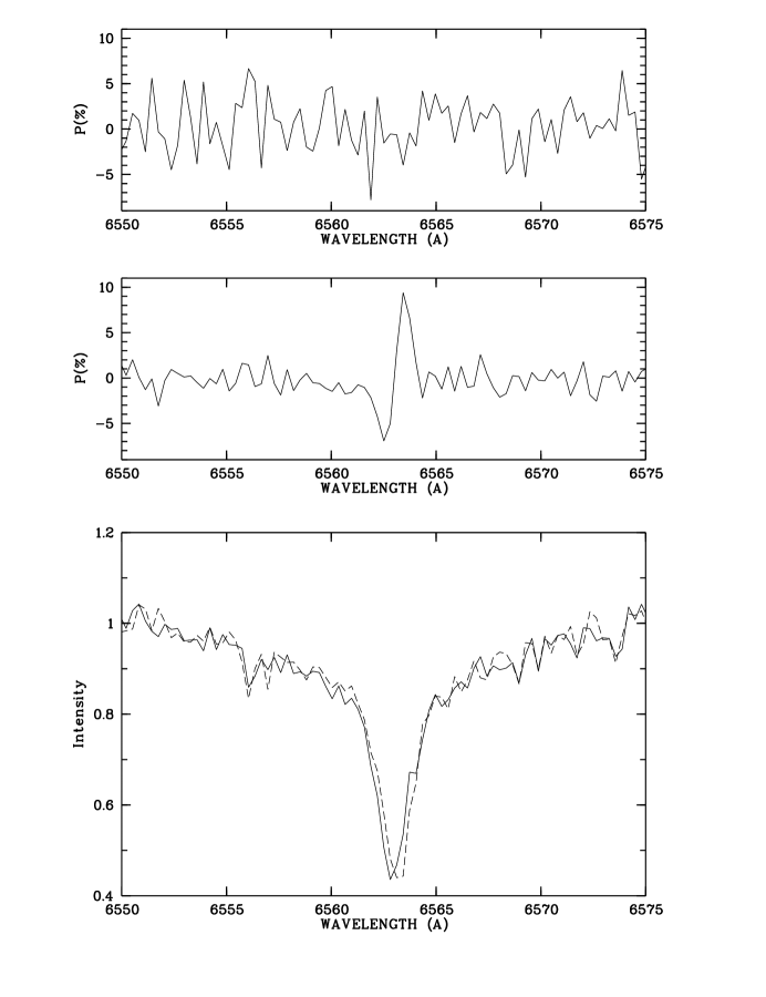
Figure 3.9: Top panel: Polarization obtained from individual spectra of the zero polarization ”cross-over point” at $0.5\pi$ or $1.5\pi$. Bottom: Two spectra of different polarization in the region of the $H\alpha$ line core. The magnetic shift is clearly visible. Middle: The result of the substraction of these spectra, i.e. Stokes $V$. From Fabrika et al. (2000) [114].

3.7 Comparison of the results

After we have obtained several upper limits on $k^{2}$ for various objects (including the sun) it is interesting to ask, whether we can find a correlation between them. For this purpose we have listed in Tab. 3.2 the masses and radii in solar units of the investigated objects, together with the corresponding highest and lowest upper limits on $k^{2}$ obtained from our analysis and their mean values in the fourth column. The last column shows the corresponding ratio $\Phi$ between the Schwarzschildradius $r_{S}=2GM/c^{2}$ of the star and its physical radius $R$, i.e. $\Phi=2GM/(Rc^{2})$.

	$M/M_{\odot}$	$R/R_{\odot}$	$k^{2}$ (km)2	$\overline{k^{2}}$ (km)2	$\Phi=2GM/Rc^{2}\,(10^{-4})$
Sun	1	1	0.69 - 1.95	1.32	0.042
40 Eri B	0.5	0.013	0.35 - 0.44	0.395	1.614
PG 2329	0.9	0.0156	0.23 - 0.28	0.255	2.42
GRW	1	0.0076	0.058 - 0.074	0.066	5.52
RE J0317	1.35	0.0035	0.036 - 0.051	0.0435	16.2

Tab.3.2: Relevant data of considered objects. First and second column: Mass and Radius in solar units. Third column: Range of upper limits on $k^{2}$ obtained from our analysis. Mean values $\overline{k^{2}}$ in the fourth column. The last column gives the ratio $\Phi$ between Schwarzschild and physical radius $\times 10^{-4}$.

The first thing which attracts attention is that the limits on $k^{2}$ decrease for increasing $\Phi$ of the stellar objects. This correlation is graphically shown in Fig. 3.10 on the next page where we plot from Tab. 3.2 the mean value of $k^{2}$ for each object against $\Phi$, marked by solid diamonds. The best fit to this distribution can be found with gaussian linear regression method. This yields

$$k^{2}(\Phi)=1.363982\cdot(\exp(-\Phi^{0.7})+0.04\,\Phi^{-0.18})\quad.$$ (3.14)

The agreement between the values $k^{2}(\Phi)$ of the fittet curve and the measured $\overline{k^{2}}$ are quite good as one can see in Tab. 3.3. Therefore, (3.14) can be interpreted in that way, that it gives approximately those upper limits on $k^{2}$ which one could expect for celestial bodies of mass $M$ and radius $R$ by using the polarization modelling technique used in this chapter. For example an object of about the mass and the size of the earth $(M_{E}=5.97\cdot 10^{24}\mbox{kg},\,R=6.378\cdot 10^{6}\mbox{m})$ would give $k^{2}_{E}\mathop{\raise 1.29167pt\hbox{$<$\kern-7.5pt\raise-4.73611pt\hbox{$\sim$}}}(1.771501\,\mbox{km})^{2}$, while a supermassive black hole similar to the one suspected in the center of our galaxy with $M_{BH}=2.5\cdot 10^{6}M_{\odot}$ and a Schwarzschildradius of $r_{S}=2GM/c^{2}=2.969\cdot 10^{9}\mbox{m}$ would give $k^{2}_{BH}\mathop{\raise 1.29167pt\hbox{$<$\kern-7.5pt\raise-4.73611pt\hbox{$\sim$}}}(0.010396\,\mbox{km})^{2}$. Finally we note that this would also be the upper limit for any other object which has reached its Schwarzschildradius, since $k^{2}_{\star}(\Phi)$ depends only on the ratio $r_{S}/R_{\star}$.

Figure 3.10: Mean value of $k^{2}$ plotted against the corresponding ratio $\Phi$ in units of $10^{-4}$. The distribution can be fitted by a smooth curve, given in the text. The different ranges of the $k^{2}$ values are of about the same size as the symbols and therefore omitted.

	$k^{2}(\Phi)$	$\overline{k^{2}}$	Deviation from $\overline{k^{2}}$ in %
Sun	1.320012	1.320	$9\cdot 10^{-4}$
40 Eri B	0.387055	0.395	2.01
PG 2329	0.259636	0.255	1.81
GRW	0.090102	0.066	36.5
RE J0317	0.034262	0.0435	21.23

Tab.3.3: Comparison of $k^{2}(\Phi)$ values from the fitted curve with the measured mean values $k^{2}$. The last column gives the relative deviation in percent of the fitted from the measured values.

3.8 Discussion and Conclusions

We have used spectropolarimetric observations of the white dwarfs Grw +70^∘8247, RE J0317-853, PG 2329+267 and 40 Eridani B to impose new strong constraints on gravitational birefringence. To improve earlier investigations of Grw +70^∘8247 we employed a dipole model for the magnetic field structure which leads to, on average, an 18% sharper limit.

However, for all white dwarfs we have considerd our constraints on $k_{\star}$ and $l_{\star}$ strongly depend on the sophisticated form of the weight function $w(\mu)$. At the moment, $w(\mu)$ only gives very conservative results from a simple relation between the magnetic field strength at a certain position on the visible stellar disc and the emitted degree of cicular polarization. So, the next step to enhance $w(\mu)$ could consist of calculating numerically the theoretical degree of circular polarization for each point on the stellar disc by using simulations of radiative transfer in stellar atmospheres. A further, clear improvement on the constraint on $k_{\star}$ should be possible within this approach.

The possibiliy, given by (3.14) to calculate approximate values for upper limits on $k^{2}$ depending on the ratio between the Schwarzschild and physical radius is certainly a useful result. Those values could be used as a guideline for the birefringence analysis of other objects. However, the constant numerical values in (3.14) possibly have to changed slightly when measured $k^{2}$ values of other objects has to be fitted into this scheme.

Chapter 4 Cataclysmic Variables

The method which we have used up to now for setting strong upper limits on gravity-induced birefringence is very limited. As mentioned before, this is mainly due to the lack of a reliable atmospheric model for magnetic white dwarf stars which could provide realistic estimates for the emitted degree of polarized radiation as a function of field strengths and opacities.

In this chapter we circumvent this restriction by focussing our attention on magnetic white dwarfs which are members in close interacting binary systems. These are systems where two stars move around the common center-of-mass in a close orbit so that matter can fall along a ballistic stream from one star to the other. An important subclass of these cataclysmic variables are the AM-Her type binary systems where the white dwarf posses a strong magnetic field so that matter is prevented from forming an accretion disc and, instead, impacts directly on the stellar surface near the magnetic poles. During this process highly polarized cyclotron radiation is emitted whose rotational modulation provides a unique opportunity not only for setting upper limits on gravity-induced birefringence but perhaps also for the very first direct observation of this effect.

We therefore begin this chapter with a brief introduction into the basic physics of close interacting binary systems. The characteristics of the polarized radiation are determined by the various parameters like the temperature structure and height of the shock front, formed when the accreting matter hits the stellar surface, as well as by the electron number density of the heated plasma and the angular extend of the emission region. A realistic estimate of the emitted degree of polarization therefore depends heavily on the quality of the shock front model. With this underlying physical structure, the theory of radiative transfer of polarized radiation in the case of cyclotron emission is reviewed. Although the theory is well known for decades now, we add a new feature by modifying the resulting Stokes vector when we allow for gravity-induced birefringence.

Using this theoretical framework we present phase dependent light and polarization curves for the AM-Her system VV Puppis which are compared with polarimetric data taken by Cropper & Warner in 1986 [135]. Although the observed asymmetries are in agreement with our numerical curves, the flat topped character seen in observations cannot be achieved numerically. However, by allowing for sufficiently strong birefringence we obtain a good conformity with the observations.

4.1 Basic model of interacting binaries

Approximately $50-60$% of all stars are assumed to be members of binary systems. By involving nearly the whole spectrum of stars from red giants to black holes as possible binary components, these systems often provide examples of astrophysical processes which are among the most exciting currently known. From a more practical point of view the most precise mass determinations in astronomy are available from binary systems where the period of revolution is precisely measurable due to mutual occultations.

The physics of binary systems depends of course on the masses of the involved stars and, more importantly, on their spatial separation. If the distance between both components is big enough so that they can interact at every evolutionary stage only gravitationally without any related mass transfer, then each member of the binary will pass through its individual development without being disturbed by its companion. An example for this is Sirius with the white dwarf Sirius B as the second star. However, the situation becomes more interesting if the stars move so close to each other that tidal effects are no longer negligible. In this chapter we are interested in such systems which consist of a white dwarf as the primary component and an, evolutionary younger and more massive, secondary component which can be represented by a main sequence or a red giant star. If both stars are not too close, their initial spherical shapes becomes teardrop-shaped with the tip pointing towards the companion. Basically a mass transfer stream between the components can now be initialized in two ways, i.e. either by an evolutionary expansion of the secondary component or by a continuous decrease of the distance between the stars. In both cases, the secondary component begins to fill its Roche lobe (the volume surrounding an object within matter is gravitationally bound to it) and matter is transfered to the primary component via the inner Lagrange point L1. The mechanism of how exactly the distance between the stars could be further decreased is not fully understood at the moment. One possibility is that they already originated in close proximity or that due to friction of the surrounding material from both components the rotational energy of the system was partially converted into internal energy.

Once the mass transfer has started, the angular momentum of the system prevents the stream from falling directly onto the white dwarf surface. Instead the material forms, in most cases, an accretion disc where the gas slowly spirals inwards while, again by friction, the gravitational energy is converted into thermal energy. Finally, the matter falls onto the white dwarf from the inner edge of the disc. However, this is not a continuous process since the material is mostly accumulated in the accretion disc until the disc becomes unstable and, then, is suddenly deflated accompanied by a huge brightening of the disc due to conversion of gravitational to thermal energy. Such an event is also known as a dwarf nova. Such close binary systems which interact by means of a mass transfer stream are called cataclysmic variables.

For our purpose, the most interesting among them are those where the white dwarf posseses a ultrastrong magnetic field of the of the order $10\mathop{\raise 1.29167pt\hbox{$<$\kern-7.5pt\raise-4.73611pt\hbox{$\sim$}}}B\mathop{\raise 1.29167pt\hbox{$<$\kern-7.5pt\raise-4.73611pt\hbox{$\sim$}}}60$ megagauss (MG), which prevents the formation of a normal accretion disc and leads, instead, to a well-defined accretion flow from the secondary component to near the magnetic pole(s) of the white dwarf. These objects are often called AM-Her systems, after the prototype AM-Herculi discovered in 1923.

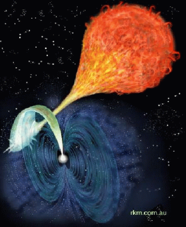
Figure 4.1: Artist impression of an Am-Her type system.

The name ”Polar” for AM-Hers and related systems was introduced by Krzeminski & Serkowski in 1977 [117] because of the strong and variable circular $(\sim 10\%-30\%\,\cite[cite]{[\@@bibref{}{cw86,tap77}{}{}]})$ and linear polarization which is typical for these objects. Certainly this attribute makes the polars very appealing for utilizing them for possible measurements of gravity-induced birefringence. Therefore, the next sections will give some insight into the basic physical processes responsible for the emission of polarized radiation. This, in turn provides the basis for a critical analysis of the observed polarization properties with respect to gravity-induced birefringence.

Figure 4.2: Schematic representation of the accretion pattern in AM Hers (adopted from Wickramasinghe & Ferrario [87]).

4.2 Mass transfer and shock models

The basic model which has been developed for AM-Her type systems is briefly sketched in Fig.4.2. It is mainly based on X-ray observations [118], modelling of the continuum and emission-line radiation from magnetically confined accretion funnels [119], and polarized emission from shocks [120].

For an ordinary, nonmagnetic primary component the matter streams from the secondary star and accumulates in a disc before impacting on the white dwarf surface. On the other hand the detailed accretion mechanisms are much more complicated and even controversial (e.g. [121]) if the primary component posseses a strong magnetic field. However, it is generally accepted that after the material has left the companion star near the inner Lagrangian point, a stream is formed which falls freely towards the white dwarf on a ballistic trajectory. If the magnetic field of the accreting object is strong enough $(\mathop{\raise 1.29167pt\hbox{$>$\kern-7.5pt\raise-4.73611pt\hbox{$\sim$}}}1$MG) the increasing magnetic pressure will begin to dominate the material flow at some distance from the white dwarf in a region called the coupling region. Here, the radial velocity component is reduced and the flow aquires first toroidal and then poloidal velocity components as the stream couples onto the field lines. From that point the material falls again freely towards the accreting object in magnetically confined funnels that connect the coupling region with the white dwarf surface. Finally a static shock above one or both magnetic poles slows and heats the infalling material before it settles on the surface with a temperature of $kT\approx 10$keV.

4.2.1 The shock region

The shock region can be regarded as the main source of emission in the optical and the X-ray wave band. Calculations of the circular polarization light curve presented in this chapter are therefore based on a sophisticated model of the emission region, first invented by Wickramasinghe & Megitt in 1985 [123].

The first attempts to model the shock fronts of AM-Her type systems, given by Meggitt & Wickramasinghe in 1982 [124], were based on the assumptions of constant temperature accretion columns. Although successful in explaining some of the gross properties like the continuum energy distribution, this model, based on cyclotron opacity, failed to predict the correct degree of polarization (the predicted values were a factor of about 2-3 higher than observed). The model which is discussed here can be regarded as a further development of this early model since it includes a temperature structure (shock front) as well as free-free opacity as a pure absorption process.

Assuming that the ionized material falls freely towards the magnetic poles, it moves a radial distance $r$ with the velocity

$$V(r)=\left(\frac{2GM}{r}\right)^{1/2}=5.2\times 10^{8}\left(\frac{M}{M_{\odot}}\right)^{1/2}\left(\frac{10^{9}\mbox{\footnotesize{cm}}}{R}\right)\left(\frac{R}{r}\right)^{1/2}\mbox{\footnotesize{cm}}\,s^{-1}\quad,$$ (4.1)

where $M$ and $R$ are the mass and the radius in (cm) of the white dwarf respectively. Before the material settles down on the surface, the density is increased in a strong shock by a factor 4 and the velocity decreases by the same factor across the shock front. In the case that this shock is formed near the white dwarf surface, the shock temperature is given by

$$T_{S}=\frac{3\mu m_{H}GM}{8kR}=6\times 10^{8}\mu\left(\frac{M}{M_{\odot}}\right)\left(\frac{10^{9}\mbox{\footnotesize{cm}}}{R}\right)\mbox{K}\quad,$$ (4.2)

where $\mu$ denotes the mean molecular weight. The postshock electron density is

$$N_{e}=3.8\times 10^{17}\left(\frac{F_{s}}{10^{2}\mbox{\footnotesize{g cm}}^{-2}s^{-1}}\right)\left(\frac{M}{M_{\odot}}\right)^{-1/2}\left(\frac{R}{R_{\odot}}\right)^{1/2}\mbox{\footnotesize{cm}}^{-3}\quad,$$ (4.3)

where $F_{s}$ is the specific accretion rate. In this context it is important to note that the scope of this model only allows accretion within a small fraction of the stellar surface namely on a point like structure. This restriction will later be removed by a more general approach that also allows for more extended shock regions.

The bulk of the translational energy is carried by the ions which achieve a Maxwellian velocity distribution by ion-ion collisions at a distance $h_{\mbox{\tiny{ion}}}\sim V_{\mbox{\tiny{ion}}}t_{\mbox{\tiny{ion}}}$, where $t_{\mbox{\tiny{ion}}}$ denotes the ion-ion collision time scale [125], while the electrons are mainly heated by Coulomb collisions with the ions. The electron temperature usually differs from the ion temperature and both vary with height in the shock [126, 127]. As the gas then settles on the stellar surface it is cooled by bremsstrahlung and cyclotron radiation. In the case that cyclotron radiation dominates, the electrons cool faster than they can be heated by collisions with ions, with the consequence that ions and electrons have different temperatures, so that the gas in the ”two-fluid” regime. However, it is important to note that the accretion flow in AM-Her systems is not continuous. Occasionally these systems drop to low states of reduced brightness which could be explained by interruptions or reductions in the material stream. The reason for this accretion modulation is not fully understood at the moment, but it may be related to solar-type magnetic activity in connection with starspots of the secondary component [122].

4.2.2 Extended emission regions

Figure 4.3: Orientation of the dipole axis $d$ and the spin axis $l_{s}$ relative to the symmetry axis $l_{p}$ of the emission region and the line-of-sight.

The idea that the emission regions are pointlike sources located at the diametrically opposite magnetic poles is insufficient and often contradicted by observations. For example the asymmetries seen in polarization light curves of most systems or the wavelength dependence of intensity and polarization in AM-Her itself are hardly reproduced by these models. Therefore, Wickramasinghe & Ferrario [132, 133] introduced emission regions which extend across and above the stellar surface. Consequently, this new concept allowed for field spread, density and temperature structure, and for displacement from the magnetic poles.

The field geometry is that of a centered dipole. Using a cartesian coordinate system, the spin axis $l_{s}$ is inclined with respect to the line-of-sight by an angle $i$ in the $y-z$-plane, while the symmetry axis of the emission region $l_{p}$ is identified with the positive $z$-axis making an angle $\Delta$ with respect to the spin axis. The emission region itself extends over a spherical cap which subtends an angle $2\alpha$ at the center of the star. In this coordinate system, the dipole axis has a polar angle $\Theta_{B}$ with $l_{p}$ and an azimuthal angle $\Phi_{B}$ with respect to a line perpendicular to $l_{p}$ in the same plane as $l_{p}$ and $l_{s}$. We can therefore identify this line with the (positive) $y$-axis of the cartesian system in the direction $l_{p}\times(l_{p}\times l_{s})$. The relative orientations of the various axes are shown in Fig.4.3.

For our purpose, the best agreement with observations was achieved by assuming uniform electron temperature $T_{e}$ and fixed electron number density $N_{e}$. The emission region has a constant radial thickness $H$ so that the characteristics of the emission region can be summarized by the optical depth parameter

$$\Lambda_{H}=2.01\times 10^{8}(H/10^{8}\mbox{\footnotesize{cm}})(N_{e}/10^{16}\mbox{\footnotesize{cm}}^{-3})(3\times 10^{7}G/B)$$ (4.4)

in the radial direction [133]. Of course $\Lambda_{H}$ varies over the emission region due to changes in $B$. The magnetic field strength $B$ in the above expression is evaluated at the magnetic pole.

4.3 Cyclotron radiation and birefringence

Since the cyclotron emission is highly polarized, the AM-Her systems provide an exellent opportunity to test for gravity-induced birefringence. For this purpose we have used a FORTRAN program, written by D.T. Wickramasinghe which calculates the Stokes vector of cyclotron emission in the ’point source’ approximation of Wickramasinghe and Meggitt [123] using a fixed electron temperature $T_{e}$ and a fixed optical depth parameter $\Lambda$. This section will present the underlying mathematical formalism with the additional new feature of a gravity-induced alteration of the Stokes vector. Extended emission regions, introduced in the previous section, are easily obtained from this concept as a homogeneous composite of pointlike sources.

Consider an electron in helical motion in a uniform magnetic field directed along the z-axis in a cartesian coordinate system. The energy emitted per unit solid angle $\Omega$ making an angle $\theta$ with the magnetic field and per frequency interval $d\omega$ is given by

$$\epsilon_{0}d\omega\,d\Omega=\frac{e^{2}\omega^{2}}{2\pi c}\sum_{n=1}^{\infty}F_{n}\delta_{n}(y)$$ (4.5)

where $\epsilon_{0}$ is also the coefficient of spontaneous emission, with

$$F_{n}=(\cot\theta-\beta_{\|}\mbox{cosec}\,\theta)^{2}J^{2}_{n}(n\xi)+\beta_{\perp}^{2}J^{{}^{\prime}2}_{n}(n\xi)$$ (4.6)

where $J_{n}$ is the Bessel function of order $n$ and $J_{n}^{{}^{\prime}}(n\xi)\equiv dJ_{n}(n\xi)/d(n\xi)$ [128]. Further, $\beta_{\|}$ and $\beta_{\perp}$ are the parallel and perpendicular components of the dimensionless velocity $\beta=v/c$, so that we define $\xi=\beta_{\perp}\sin\theta/(1-\beta_{\|}\cos\theta)$. The argument of the $\delta$ function is

$$y=n\omega_{c}/\gamma-\omega(1-\beta_{\|}\cos\theta)$$ (4.7)

where $\omega_{c}=eB/mc$ is the electron cyclotron frequency and $\gamma=(1-\beta^{2})^{-1/2}$ the usual Lorentz factor. From this one can easily see, that the radiation spectrum consists of spectral lines occuring at frequencies

$$\omega=\frac{n\omega_{c}}{\gamma(1-\beta_{\|}\cos\theta)}\quad,$$ (4.8)

which also gives a relation between $\gamma$ and harmonic number $n$.

In order to describe a uniform plasma with temperature $T$ and electron number density $N$, one has to introduce a relativistic Maxwellian distribution in (4.5) and integrate over $\beta_{\|}$

$$\epsilon_{I}\,d\omega\,d\Omega=\frac{e^{2}\omega^{2}}{4\pi c}\frac{N\mu}{K_{2}(\mu)}\sum_{n=1}^{\infty}\int_{-1}^{1}F_{I}\exp(-\mu\gamma)(\gamma^{4}/n\omega_{c})d\beta_{\|}\,d\omega\,d\Omega$$ (4.9)

where the dimensionless electron temperature $\mu=mc^{2}/kT$ serves as the argument of the modified Bessel function of the second kind, $K_{2}(\mu)$.

To obtain the emission coefficients $\epsilon_{Q}$ and $\epsilon_{V}$ for Stokes $Q$ and Stokes $V$, one defines a coordinate system where the z-axis serves as the line-of-sight and the uniform magnetic field lies in the x-z plane, making an angle $\theta$ with the z-axis. Then, the complex Jones vector for the electric field of the radiation of a single electron is proportional to ([128])

$$\left(\begin{array}[]{c}(\cot\theta-\beta_{\|}\mbox{cosec}\,\theta)J_{n}(n\xi)\\ -i\beta_{\perp}J^{{}^{\prime}}_{n}(n\xi)\\ 0\end{array}\right)\quad.$$ (4.10)

The emission coefficients $\epsilon_{Q}$ and $\epsilon_{V}$ for the Stokes parameters $Q$ and $V$ are obtained by replacing $F_{I}$ in (4.9) with

$$F_{Q}=(\cot\theta-\beta_{\|}\mbox{cosec}\,\theta)^{2}J^{2}_{n}(n\xi)-\beta_{\perp}^{2}J^{{}^{\prime}2}_{n}(n\xi)$$ (4.11)

and

$$F_{V}=-2(\cot\theta-\beta_{\|}\mbox{cosec}\,\theta)J_{n}(n\xi)\beta_{\perp}J^{{}^{\prime}}_{n}(n\xi)$$ (4.12)

respectively, while $\epsilon_{U}=0$. Since $0\leq\xi\leq 1$ the Bessel function $J_{n}$ and its derivative can be replaced with the Wild-Hill approximations [105] which are more easy to implement in a computer program

$$J_{n}(n\xi) \approx \frac{\xi^{n}\exp(nw)}{\sqrt{2\pi n}(1+w)^{n}}[w^{3}+0.5033/n]^{-1/6}$$ (4.13)

$$J^{{}^{\prime}}_{n}(n\xi) \approx \frac{\xi^{n-1}\exp(nw)}{\sqrt{2\pi n}(1+w)^{n}}[w^{3}+1.193/n]^{1/6}[1-1/5n^{2/3}]$$ (4.14)

with $w=\sqrt{1-\xi^{2}}$. The cyclotron absorption coefficients are given by Kirchhoff’s law, since the electrons are in thermal equilibrium, i.e.

$$\epsilon_{I}=\kappa_{\mbox{\tiny{cyc}}}B_{\omega},\quad\epsilon_{Q}=q_{\mbox{\tiny{cyc}}}B_{\omega},\quad\epsilon_{V}=v_{\mbox{\tiny{cyc}}}B_{\omega},$$ (4.15)

with the Rayleigh-Jeans law

$$B_{\omega}=\omega^{2}kT/4\pi^{3}c^{2}\quad.$$ (4.16)

In contrast to the first model, given by Meggitt & Wickramasinghe in 1982 [124] the new scheme also includes free-free opacity as a pure absorption process. The corresponding opacities are

$$\kappa_{\mbox{\tiny{ff}}} = \frac{\omega_{p}^{2}(2\omega^{4}+2\omega^{2}\omega_{c}^{2}-3\omega^{2}\omega_{c}^{2}\sin^{2}\theta+\omega_{c}^{4}\sin^{2}\theta)}{2c\omega^{2}(\omega^{2}-\omega_{c}^{2})^{2}}\,\nu_{c}$$ (4.17)

$$q_{\mbox{\tiny{ff}}} = \frac{\omega_{p}^{2}\omega_{c}^{2}\sin^{2}\theta(\omega_{c}^{2}-3\omega^{2})}{2c\omega^{2}(\omega^{2}-\omega_{c}^{2})^{2}}\,\nu_{c}$$ (4.18)

$$u_{\mbox{\tiny{ff}}} = 0$$ (4.19)

$$v_{\mbox{\tiny{ff}}} = \frac{2\omega_{p}^{2}\omega\omega_{c}\cos\theta}{c\omega^{2}(\omega^{2}-\omega_{c}^{2})^{2}}\,\nu_{c}$$ (4.20)

with the plasma frequency $\omega_{p}=(4\pi N_{e}e^{2}/m)^{1/2}$ and the approximately collision frequency $\nu_{c}=3.63N_{e}T^{-3/2}\ln(2.95\times 10^{11}T/\omega)$. It is assumed that the opacity can be treated as a sum of cyclotron and free-free components, hence

$$\kappa=\kappa_{\mbox{\tiny{cyc}}}+\kappa_{\mbox{\tiny{ff}}},\quad q=q_{\mbox{\tiny{cyc}}}+q_{\mbox{\tiny{ff}}},\quad v=v_{\mbox{\tiny{cyc}}}+v_{\mbox{\tiny{ff}}}\quad.$$ (4.21)

The transfer equation now becomes

$$\frac{d}{ds}\left(\begin{array}[]{c}I\\ Q\\ U\\ V\end{array}\right)=\left(\begin{array}[]{c}\epsilon_{I}\\ \epsilon_{Q}\\ 0\\ \epsilon_{V}\end{array}\right)+\left(\begin{array}[]{cccc}-\kappa&-q&0&-v\\ -q&-\kappa&-f&0\\ 0&f&-\kappa&-h\\ -v&0&h&-\kappa\end{array}\right)\left(\begin{array}[]{c}I\\ Q\\ U\\ V\end{array}\right)$$ (4.22)

with the Faraday mixing coefficients

$$f = (\omega_{p}^{2}/c\omega_{c})\cos\theta/(\omega^{2}/\omega^{2}_{c}-1)$$ (4.23)

$$h = (\omega_{p}^{2}/c\omega_{c})\sin^{2}\theta/2(\omega^{3}/\omega^{3}_{c}-\omega/\omega_{c})\quad.$$ (4.24)

For uniform conditions these coefficients are constant along a ray. In order to solve the transfer equation (4.22) set

$$m = 0.5(f^{2}+h^{2}),\,n=0.5(q^{2}+v^{2}),\,p=qf-vh,\,r=qh+vf,$$ (4.25)

$$R = [(m+n)^{2}-p^{2}]^{1/2},\,a_{1}=(m+n+R)/p,\,a_{3}=1/a_{1},$$ (4.26)

$$\lambda = (n-m+R)^{1/2},\,\mu=(m-n+R)^{1/2},$$ (4.27)

$$b_{1} = (f-qa_{1})/\lambda,\,b_{3}=(f-qa_{3})/\mu$$ (4.28)

$$c_{1} = -(h+va_{1})/\lambda,\,c_{3}=-(h+va_{3})/\mu\quad.$$ (4.29)

Setting all intensities equal to zero at $s=0$, the Stokes parameters of the radiation after passing through a distance $s$ are (see [124])

$$I/B_{\omega} = 1-(p/2R)(a_{1}\cosh\lambda s-a_{3}\cos\mu s)\exp(-\kappa s),$$ (4.30)

$$Q/B_{\omega} = -(p/2R)(b_{1}\sinh\lambda s-b_{3}\sin\mu s)\exp(-\kappa s),$$ (4.31)

$$U/B_{\omega} = (p/2R)(\cosh\lambda s-\cos\mu s)\exp(-\kappa s),$$ (4.32)

$$V/B_{\omega} = -(p/2R)(c_{1}\sinh\lambda s-c_{3}\sin\mu s)\exp(-\kappa s)\quad.$$ (4.33)

The question of how gravitational birefringence could be implemented in this scheme depends heavily on the shock height above the stellar surface where the polarized radiation is emitted. Since the phase shift $\Delta\Phi$ in (1.61) is proportional to $1/R$ where $R$ denotes the radial distance from the stellar center, an emission region which is extended of approximately one stellar radius above the surface would require an integration process along the shock height where a gravitationally modified transfer equation has to be solved for each plane parallel slab. An upper limit on the shock height is given in the ’single-fluid’ approximation when bremsstrahlung is the dominating cooling mechanism. In this case the height $h_{\mbox{\tiny{br}}}$ is simply proportional to the product between the free-fall velocity $V_{\mbox{\tiny{ff}}}$ (the index ’ff’, of course, must not be confused with the index for free-free absorption) and the specific cooling time $t_{\mbox{\tiny{ff}}}$ for electrons due to bremsstrahlung. The explicit expression for $h_{\mbox{\tiny{br}}}$, given by Wickramasinghe & Ferrario [87] is

$$h_{\mbox{\tiny{br}}}=9.6\times 10^{7}\left(\frac{10^{16}\mbox{\footnotesize{cm}}^{-3}}{N_{e}}\right)\left(\frac{M}{M_{\odot}}\right)\left(\frac{10^{9}\mbox{\footnotesize{cm}}}{R}\right)\,\mbox{\footnotesize{cm}}\quad.$$ (4.34)

Assuming a white dwarf mass of $M_{\odot}$ with a corresponding radius of $0.014\,R_{\odot}$ this yields a height of $\sim 10^{8}$cm with $N_{e}=10^{15}$. Since we focus on a ’two-fluid’ model when the electrons are cooled by cyclotron radiation, this means that we have for the cooling time $t_{\mbox{\tiny{cyc}}}\ll t_{\mbox{\tiny{ff}}}$ and, therefore, $h_{\mbox{\tiny{cyc}}}\ll h_{\mbox{\tiny{br}}}$. For this reason it is justified to view the polarization as emitted from near the surface because $h_{\mbox{\tiny{cyc}}}\ll 10^{2}$km is certainly a sufficient upper limit. We can therefore assume that birefringence acts directly on (4.32) and (4.33) according to

$$\left(\begin{array}[]{c}U_{\mbox{\tiny{grav}}}\\ V_{\mbox{\tiny{grav}}}\end{array}\right)=\left(\begin{array}[]{cc}\cos\Delta\Phi&0\\ 0&\cos\Delta\Phi\end{array}\right)\left(\begin{array}[]{c}U_{\mbox{\tiny{cyc}}}\\ V_{\mbox{\tiny{cyc}}}\end{array}\right)\quad.$$ (4.35)

Our objective is to include birefringence given by these equations in the calculations of synthetic polarization light curves from AM-Her type systems. In this way we can set sharp upper limits on this effect with a new method, independent from techniques presented in chapter two.

4.4 Polarimetry of VV Puppis

VV Puppis serves as a key system for our purpose of either detecting weak gravitational birefringence or setting strong upper limits on it by means of gravitationally modified polarization curves. We therefore present here some of the most important results that have been achieved for this system within the last decades and which provide the basis for the subsequent analysis.

VV Puppis was discovered in 1931 by van Gent [129] as a faint $(V=14.5-18)$ variable with a period of 100 min. Sinusoidal variations in radial velocity of the H and He II line, correlated with the 100 min photometric variation led Herbig in 1960 to the conclusion that the observations could best be explained by means of a binary system where the emission lines originate on the brighter (primary) component [130]. Herbig also concluded that changes in the shape of the light curve could have its origin in variations of the emission area on the visible stellar surface which can be realized by self eclipses of the relevant area due to rotation. This picture was refined in 1977 by Tapia’s discovery of strong linear and circular polarization with a maximum of $\sim 16$%[116] in each polarization state of the optical light curve, confirming the suggestion by Bond and Wagner (IAUC 3049) that this object is similar to the ”original” AM-Her system. Two years later, Visvanathan and Wickramasinghe identified a series of absorption features in the spectrum with the 6th, 7th and 8th harmonics of cyclotron absorption in a nearly uniform magnetic field of $\sim 3\cdot 10^{7}$G. This discovery renewed the general interest in astrophysical cyclotron emission models, since it was the first detection of resolvable cyclotron harmonics in the optical spectrum of a stellar object. However, these results had an uncertainty of one harmonic in the identification since the observed features did not have well defined cores. As a consequence the corresponding uncertainty in $B$ was $\sim 20$%. Concerning the visibility of cyclotron harmonics, numerical computations, based on the calculations presented in section 4.3 revealed that very special conditions are required to produce consistency with the observed spectrum [132].

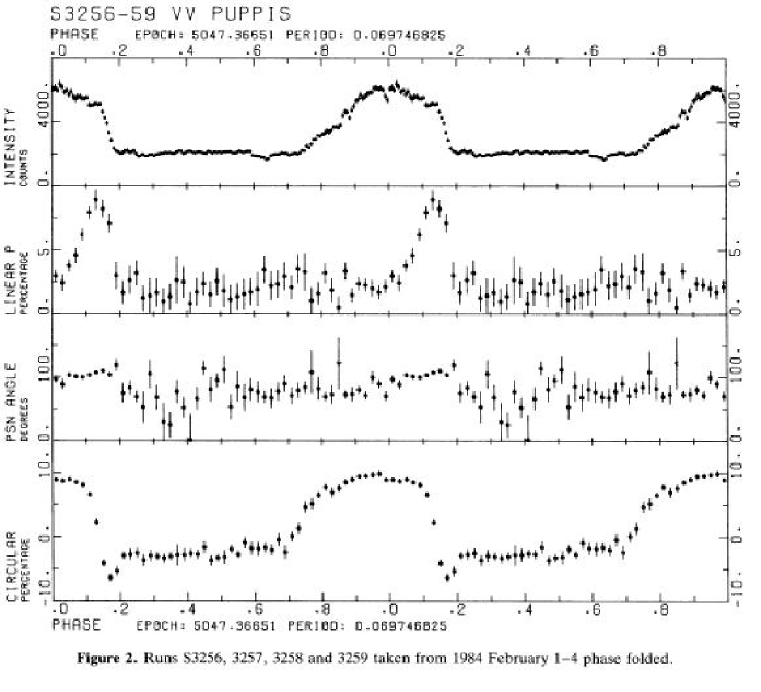
Figure 4.4: Intensity and polarization light curves of VV Puppis. From: Copper & Warner (1986) [135].

For the shock front model related to VV Puppis one can therefore conclude a viewing angle $i\sim 70^{\circ}-90^{\circ}$ with respect to the magnetic field, low optical depths $\Lambda\sim 10^{5}$ and high temperatures of $T\sim 10$ keV in a magnetic field of $\sim 3\cdot 10^{7}$G. The fact that VV Puppis is the only stellar object to show resolvable cyclotron harmonics in its optical spectrum is difficult to explain, although it might be possible that magnetic field broadening often renders the features undetectable [132].

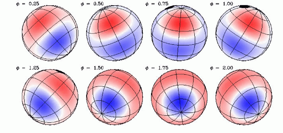
Figure 4.5: Visualization of the longitudinal magnetic field components of VV-Puppis during successive rotational phases. The black spot which is visible from $\phi\approx 0.75$ to $\phi\approx 1.25$ markes the position of an emission region with size $\alpha=10^{\circ}$ and displacements $\Phi_{B}=90^{\circ}$, $\Theta_{B}=30^{\circ}$ from the dipolar axis.

Fig.4.4 shows phase dependend, wavelength averaged polarization curves of VV Puppis from Cropper & Warner (1986) [135]. As one can see, the light curves are strongly modulated at the orbital period and the accreting pole is visible only for $\sim 40$% of the period. A common feature is the slow rise after eclipse egress and a more rapid decline before eclipse ingress. Although linear polarization is present during the entire bright phase, with a second, lower peak at phase 0.7, the strong linear polarization peak of $\sim 9$% is expected to be caused by a magnetic field configuration that can be seen only briefly at a viewing angle of $\sim 90^{\circ}$ with respect to the line-of-sight. In this case linear polarization due to cyclotron radiation is strongest and would therefore explain the observed feature. The circular polarization reaches a maximum value of $\sim 10$% during the bright phase after a more gradual rise. The steeper descent of the circular polarization is followed by a sign reversal and a short dip, lasting 0.05 of a cycle. One of the most important results is that VV Puppis shows steady negative circular polarization throughout the entire eclipse phase, which could be explained by accretion onto a second region of the white dwarf [136], that is visible at all rotation phases [137]. However, the negative polarization dip at eclipse ingress is probably related to the shape of the primary accretion region. This conjection is supported by synthetic light curves of only one accretion region as we will later show.

On the basis of the light curves in Fig.4.4, Cropper & Warner reported for the system geometry an inclination of $i=77^{\circ}\pm 7^{\circ}$ and a magnetic colatitude of $\Delta=155^{\circ}\pm 6^{\circ}$. In 1987 Wickramasinghe & Ferrario used $i=75^{\circ}$ and $\delta=150^{\circ}$ for the calculation of phase dependent light curves of a displaced accreting pole. Fig.4.5 shows a visualization of the longitudinal magnetic field component during a rotation cycle of VV Puppis. The emission region with size $\alpha=10^{\circ}$ has an azimuthal and polar angle of $\Phi_{B}=90^{\circ}$ and $\Theta_{B}=30^{\circ}$, respectively, marked by the black spot. One can see that in this configuration the emission region merely grazes the limb during the bright phase, which is extraordinarily useful for our purpose, since gravitational birefringence is most pronounced for sources located at the stellar limb. Further, the asymmetry in the linear pulse and the sign reversal in circular polarization, prior to eclipse ingress can now be explained by means of the system geometry. Calculating the angles $\theta$ between the field directions in the spot and the line-of-sight one finds, that the angles are mostly greater than $90^{\circ}$ at eclipse ingress and mostly less than $90^{\circ}$ at eclipse egress. The observed reversal in the sign of circular polarization occurs just shortly before eclipse ingress when $\theta>90^{\circ}$ while the stronger linear pulse as well as the maximum intensity occurs at $\theta\approx 90^{\circ}$ as expected from the beaming properties of cyclotron radiation.

4.4.1 Gravitationally modified lightcurves

The programm which we have developed for calculations of gravitationally modified polarization curves is based on a FORTRAN routine written by D.T. Wickramasinghe which calculates cyclotron emission in the ”point source” approximation of Wickramasinghe & Meggitt [123] for fixed optical depth parameter $\Lambda$ and fixed electron temperature. Since the point source approximation is insufficient to account for most of the observed polarization curve characteristics as explained in section 4.2.2, our code describes an extended emission region as a composition of $\sim 3\times 10^{2}$ point sources, depending on the size of the emission region. This emission region is placed on a rotating sphere according to the coordinate system described in sect. 4.2.2, so that the polarization values (circular and linear) taken at each rotational phase yields the final polarization curve.

We first present light curves without gravitational modification in order to have a comparison to the observed curves of Cropper & Warner [135]. Fig.4.6 shows the phase dependent polarization and light curves for two different models. While both models have the same inclination $i=75^{\circ}$ and magnetic colatitude $\Delta=150^{\circ}$ for the position of the spot, the left column shows the curves for polar cap size $\alpha=5^{\circ}$ and a dipole axis orientation with $\theta_{B}=10^{\circ}$ and $\Phi_{B}=90^{\circ}$. The curves in the right column have $\alpha=10^{\circ}$, $\theta_{B}=30^{\circ}$ and $\Phi_{B}=90^{\circ}$. We take note that these curves are in good agreement with the curves presented by Wickramasinghe & Ferrario in 1988 [133] (hereafter WF88) for extended emission regions using similar parameters. At this point it is important to note, that these curves (including those in WF88 [134]) require an additional constant background of unpolarised light in order to reproduce observations at least approximately. This constant, unpolarized continuum probably comes from a component of the binary system which is always visible, like the accretion stream, white dwarf photosphere or something similar - up to now the genuine origin is unknown as well as how to correctly estimate it. Currently the only restriction is placed by the observed polarization levels and, so, the continuum has to be introduced by hand to get the observed levels right.

Since our code only allows for emission from one pole, the circular polarization curve does not show a constant negative polarization throughout the hole period which is seen in the observations. Basic characteristics like the asymmetry in the linear pulse and the negative dip in circular polarization prior to eclipse ingress stand comparison to what is observed by Cropper & Warner. Nevertheless we note that the observations shows a more gradual rise in intensity and polarization whereas the rapid declines are in agreement with our models.

These ”pure” curves (without any birefringence influence) could possibly better fitted to observations by a different geometrical shape of the emission region. While the present curves are based on a cylindrical symmetric source, a more elongated, arc-like structure could perhaps account for the observed gradual rise. Observational hints for arc-like emission regions has been presented by Beuermann et al. in 1987 [138] and also by Cropper [139]. We will come to this point again after the discussion of the gravitationally modified polarization curves. In accordance with WF88 we emphasize that the characteristics of the polarization curves depend sensitively on $\Phi_{B}$ for a given $\alpha$ and $\theta_{B}$. For instance, for $\Phi_{B}=0^{\circ}$ we obtain no polarization reversals while for $\Phi_{B}=180^{\circ}$ we observed two symmetrical reversals at eclipse ingress and eclipse egress.

Figure 4.6: Phase dependent circular polarization curve of VV Puppis for an emission region centered at latitude $\Delta=150^{\circ}$. The orbital inclination is $i=75^{\circ}$ and $\omega/\omega_{c}=6.2$. The curves in the left column correspond to $\alpha=5^{\circ}$ and $\theta_{B}=10^{\circ},\,\Phi_{B}=90^{\circ}$, while the right column corresponds to $\alpha=10^{\circ}$ and $\theta_{B}=30^{\circ},\,\Phi_{B}=90^{\circ}$.

One of the main problems that these curves and also the curves presented by WF88 have is the sinusoidal form of the circular polarization and intensity, in contrast to what is observed. For this reason it is certainly interesting to see how gravity-induced birefringence modifies the circular polarization curve. Fig.4.7 on the next page shows the phase dependent circular polarization using the same system parameters as in Fig.4.6 and $M_{\star}=0.4\,M_{\odot}$, $R_{\star}=0.014\,R_{\odot}$ but this time additionally with increasing values of the metric-affine coupling constant $k$. As expected, for $k^{2}=0$ the curves are identical with the unmodified polarization regime while for a sufficiently big $k^{2}$, the light is almost completely depolarized. In between these two ”boundary” states, one can adjust $k^{2}$ to a value $(0.13\,\mbox{km})^{2}\leq k^{2}\leq(0.14\,\mbox{km})^{2}$ so that the circular polarization curve is nearly flatten as seen in observations. At the same time, the negative dip which arises prior to eclipse ingress is only marginally influenced by birefringence, although it but also decreases somewhat with increasing $k^{2}$.

In order to see if this range for $k^{2}$ is in agreement with upper limits, derived with the methods of the chapter 3, we have made two consistency checks. By using the oblique dipolar rotator technique we got an upper limit of $k^{2}_{VV\,Pup}\leq(0.35\,\mbox{km})$ for VV Puppis without limb darkening and $k^{2}_{VV\,Pup}\leq(0.42\,\mbox{km})$ with maximum limb darkening and an observed polarization level of 10%. These limits are similar to those of 40 Eridani B from the previous chapter, i.e. $k^{2}_{40\,Eri\,B}\leq(0.35\,\mbox{km})$ and $k^{2}_{40\,Eri\,B}\leq(0.44\,\mbox{km})$, respectively with $M_{40\,Eri\,B}=0.5M_{\odot}$ and $R_{40\,Eri\,B}=0.0136\,R_{\odot}$ comparable to $M_{VV\,Pup}=0.4M_{\odot}$ and $R_{VV\,Pup}=0.014\,R_{\odot}$. The other white dwarfs of chapter 3 have higher masses and/or smaller radii so that their upper values on $k^{2}$ are correspondingly lower. The same is true for the $k^{2}$ value of the sun. However, one has to note that this dipolar rotator technique assumes that the emitted degree of polarization is direct proportional to the longitudinal magnetic field strength, whereas we have seen that this relation becomes much more complicate in the case of cyclotron radiation. It is therefore more reliable to use the ”plain” model proposed by Solanki, Haugan and Mann in 1999 [86] which assumes that the polarized radiation is emitted homogeneously over the visible stellar surface. Since this is a rather conservative restriction the resulting upper limit is congruously $k^{2}\leq(0.4\,\mbox{km})^{2}$. Nevertheless it is important that the range of $k^{2}$-values for VV Puppis is consistent with the limits from the dipolar rotator model as well as with the plain model.

Since the amount of Stokes $U$ in the linear polarization signal is always $\mathop{\raise 1.29167pt\hbox{$<$\kern-7.5pt\raise-4.73611pt\hbox{$\sim$}}}5$% the linear polarization curve is hardly affected by gravity-induced birefringence which only acts on Stokes $V$ and Stokes $U$ as one can see in Fig.4.8. Nevertheless, the first smaller peak becomes sharper and more pronounced for $\alpha=5^{\circ}$ while for $\alpha=10^{\circ}$ the peak is washed out.

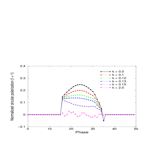
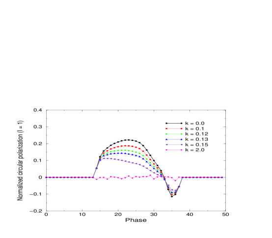
Figure 4.7: Gravitationally modified, phase dependent cicular polarization curves. The physical parameters are the same as in Fig.4.6. Upper curves: $\alpha=5^{\circ}$, $\theta_{B}=10^{\circ},\,\Phi_{B}=90^{\circ}$. Lower curves: $\alpha=10^{\circ}$, $\theta_{B}=30^{\circ},\,\Phi_{B}=90^{\circ}$.

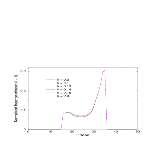
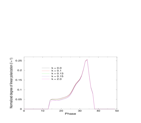
Figure 4.8: Gravitationally modified, phase dependent linear polarization curves. The physical parameters are the same as in Fig.4.6. For comparison the same $k$-values as for circular polarization have been plotted. Upper curves: $\alpha=5^{\circ}$, $\theta_{B}=10^{\circ},\,\Phi_{B}=90^{\circ}$. Lower curves: $\alpha=10^{\circ}$, $\theta_{B}=30^{\circ},\,\Phi_{B}=90^{\circ}$.

4.5 Comparison of the results

Finally, we want to check how the limits on $k^{2}$ for VV-Puppis, obtained by lightcurve fitting and the polarization modelling technique from chapter 3 fit into the empirical scheme, given by (3.14). For this purpose, Fig. 4.9 shows again the curve from Fig. 3.10 additionally with the $k^{2}_{VV\,Pup}$ values, obtained in this chapter.

Figure 4.9: $k^{2}(\Phi)$ curve of chapter 3 together with the VV Puppis limits. The upper star $(0.6|0.385)$ marks the limit obtained by the polarization modelling technique. The lower star $(0.6|0.15)$ marks the limit from lightcurve fitting. A better fit to the VV Puppis value is provided by the dashed curve.

The limit which is obtained by the polarization modelling technique deviates slightly from the curve. Nevertheless the fitting can be improved with a minimally different function

$$k^{2}(\Phi)=1,026262\cdot(\exp(-\Phi^{1.1})+0.1\,\Phi^{-0.18})\quad,$$ (4.36)

which yields the dashed line in the above figure. The bigger deviation of the lower point $(0.6|0.15)$ from the curve is not surprising, since its intention is not to serve as an upper but as a lower limit on $k^{2}$. Certainly more datapoints measured at different celestial bodies are needed to see which curve can best approximate the upper limits on $k^{2}$.

4.6 Conclusions

The main difference between the results of this chapter and those of chapter 3 is obvious. While for ”ordinary” magnetic white dwarfs we merely set upper limits on $k^{2}$ we now additionally have to assume a lower bound on $k^{2}$ in order to link the presented theory of cyclotron radiation in AM-Her type systems with observations. However one has to be very careful when making an interpretation of these results since the underlying model of interacting binary systems is afflicted by many uncertainties:

1. The fact that a constant unpolarized continuum background has to be introduced by hand to reproduce observations is unsatisfactory. A certain aspect of the physics of binary systems is therefore probably not understood and although it is rather unlikely that this aspect could lead to a modification of the present lightcurves similar to the gravitationally modified curves, it cannot be completely ruled out.

2. More importantly, Wickramasinghe & Ferrario [140] have shown that an arc-shaped emission region is also able to replace the sinusoidal shape seen in the circular polarization curve by a flat top.

At a first glance, the second point seems to discard any claim for a lower bound on $k^{2}$. Indeed, we are here confronted with two alternative models which try to explain the same observed polarization properties with different approaches. Currently there is no reliable and convincing possibility to judge in favour of one or the other approach. Although the agreement of the conventional approach with observations seems to be very appealing, the new question which now arises is, if the assumption of an arc-shaped emission region for VV-Puppis is justified any longer, taking into account the new results from gravitational birefringence. One of the main arguments supporting the arc-shaped emission regions is the flat top character of the calculated circular polarization curve as well as the correctly predicted degree of polarization - both also provided by gravity-induced depolarization. Concerning future projects it is therefore highly desirable to look for specific predictions of the conventional model which do not involve polarized radiation and are, as a result, not affected by birefringence.

However, as an important conclusion of this chapter we can say that, as long as gravitational birefringence cannot be excluded, the interpretation of polarized radiation from compact astrophysical objects is always afflicted with many uncertainties since the real nongravitational source properties may be hidden behind a birefringent curtain.

Chapter 5 Future Projects

Since astronomical tests of the Einstein equivalence principle with respect to gravitational birefringence are a relatively new area of research, we are left with several promising but so far unexplored ideas which have the potential not only for setting sharp upper limits on this effect but also for possible direct detections. We present in this chapter a selection of two elaborated but not yet finished examples where gravity-induced birefringence could either serve as a possible important contribution for a satisfying interpretation of current data or could show up as a new effect in atomic spectra under certain conditions.

The first example is concerned with the problem of circular polarization from active galactic nuclei (AGN). Under the reasonable assumption that synchrotron radiation is the main source for polarized radio emission, the degree of circular polarization measured in those AGN is on average an order of magnitude higher than expected from synchrotron theory. The suggested classical solution in terms of circular repolarization is not free from contradictions which leads to the conclusion that a gravity-induced crosstalk between linearly and circularly polarized light could provide an important contribution for solving this puzzle. The second example is concerned with gravitational red shift measurements in nonmetric theories of gravity. While in metric theories of gravity the ticking rates of (atomic) clocks are independent on their internal structure, i.e. the red shift is universal, this universality is violated for clocks which are affected by nonmetric gravitational fields. Defining three atomic clocks by different transitions of hydrogen one gets three different red shift predictions which could be tested in astronomical spectra of compact objects or under well defined laboratory conditions.

In the last part of this chapter we briefly discuss two further ideas for promising future projects. We suggest to compare the polarization properties of multiple images generated by gravitational lenses to look for traces of gravity-induced alterations due to the propagation of light through different gravitational potentials. The last issue picks up the current controversy about an intrinsic anisotropy of space time where the underlying data could be explained in terms of cosmological birefringence.

5.1 Circular Polarization of AGN

Active galactic nuclei (AGN) are characterized by a huge variety of high energy phenomena and nonthermal radiation processes which cannot be ascribed to normal stellar activity. Instead it is commonly accepted, that the main central engine is driven by a super-massive black hole, whose strong gravitational field in combination with magnetic fields and relativistic jets feeds the processes which supply the kind of radiation which is central to our current investigation. Of special interest are in this regard the compact, extragalactic radio sources which belong to the class of active galaxies. Typical representatives are Quasars and BL Lac objects, named after the prototype BL-Lacertae with strong, variable polarization and weak emission lines (Blazar). A further important example is provided by our own galaxy with the central radio source in Sagittarius A*. The optical brightness of all these objects is often clearly exceeded by emission in the radio regime with a nonthermal spectrum and non-zero degrees of polarization.

The most plausible, dominant mechanism for such radio emission in AGN is usually considered to be synchrotron radiation from an ensemble of relativistic electrons. Concerning the often differently used notations it is important to mention, that usually the name cyclotron radiation is reserved for emission from low-energy electrons whereas synchrotron radiation traditionally describes emission from highly relativistic electrons because it was first observed in 1948 in electron synchrotrons. While it is usual to use the notion ’cyclotron radiation’ with respect to magnetic white dwarfs without regarding different energies, the traditional distinction between cyclotron and synchrotron radiation is used in most of the relevant literature concerning AGN and therefore also used here.

Our special interest in this context applies to the origin of circular polarization observed in only a few AGNs. Analysis of the collation of circular polarization data presented by Weiler and De Pater in 1983 [141] revealed that out of 50 radio galaxies and 43 quasars, circular polarization was detected for only 6 radio galaxies and 15 quasars. Although at a first glance it seems very likely that a synchrotron process has to be considered as the source, the small degrees of circular polarization observed in many AGN has a frequency dependence and time variability that is not consistent with the simple predictions based on the intrinsic polarization of synchrotron emission (see [142] also for a huge list of references). Likewise the observed degrees of circular polarization are often indeed small but nevertheless too high for a simple synchrotron source. It was therefore suggested that the circular polarization is due to a propagation effect where the elliptic eigenmodes of a relativistic plasma effects cyclic conversion of linear polarization into circular polarization [143]. However, this approach is again not free of difficulties so we suggest that a conversion mechanism due to gravitational birefringence might solve these problems and contribute a significant fraction to the observed circular polarization.

In the following we give a brief overview on some of the relevant data, mainly focussed on observations of the galactic center in Sagittarius A* (Sgr A*) and discuss the conventional, propagation induced polarization mechanisms. We outline the idea how gravity-induced birefringence could account for the observed polarization.

5.1.1 Polarization properties of synchrotron emission

Following the current understanding, the radio emission of AGN is mainly produced by highly relativistic electrons which move on helical paths along magnetic field lines. A single electron moving with the synchro-cyclotron frequency $\omega_{c}$ emitts its radiation in a narrow cone of half-angle $\gamma^{-1}$ along the instantaneous trajectory, where $\gamma$ denotes the usual Lorentz factor. For a distant observer this gives a continuous spectrum with a peak at the frequency $\omega_{m}\propto\gamma^{3}\omega_{c}$. Considering an isotropic and homogeneous ensemble of relativistic electrons within a magnetic field having a power-law energy distribution such that the particle density between $E$ and $E+dE$ can be written as $N(E)\,dE\propto E^{-\Gamma}dE$, one finds that the total intensity observed from the source is $I(\nu)\propto a(\Gamma)(B\sin\theta)^{(\Gamma+1)/2}\nu^{-(\Gamma-1)/2}$, where $a(\Gamma)$ is a slowly varying function of $\Gamma$ and $\theta$ denotes the pitch angle with respect to the magnetic field. The spectral energy distribution, i.e. the dependence of intensity $I_{\nu}$ or flux $F_{\nu}$ on the frequency can often be approximated by a power law $I_{\nu}\propto\nu^{-\alpha}$ at least over limited frequency ranges. The exponent $\alpha$, called the spectral index is related to $\Gamma$ by $\Gamma=2\alpha+1$.

In the optically thin case, the polarization plane is perpendicular to the projected magnetic field with a linear polarization degree of $m_{L}=(\Gamma+1)/(\Gamma+7/3)$. In the optically thick regime, the total intensity spectrum reaches a $\nu^{5/2}$ dependency, while the degree of linear polarization now becomes $m_{L}=3/(6\Gamma+13)$, with the electric vector being maximum parallel to the projected field. The degree of linear polarization can reach theoretically up to $\sim 70$% but this high level is only rarely observed. Currently, there are two accepted mechanisms which can cause depolarization: Unresolved inhomogenities within the source and the presence of Faraday rotation internal to the source. The last point will be discussed in more detail later.

Besides linear polarization, the theory of synchrotron radiation predicts that there should also be a small amount of circular polarization [148]. Considering again a single electron gyrating in a magnetic field ${\bf B_{0}}$ which is directed along ${\bf k}$, the circular polarization is right-handed when the direction of motion passes close to the line-of-sight (LoS) on the opposite side of ${\bf B_{0}}$, while it is left-handed if it passes close to the LoS on the same side as ${\bf B_{0}}$. Therefore, in an ensemble of electrons with an isotropic distribution of pitch angles one finds approximately as many electrons contributing to right- and left-handed polarization within the emission cone so that, to first order, the circular polarization cancels out, leaving the emission linearly polarized. However, Legg & Westfold [148] proposed that the total emission from an ensemble of gyrating electrons could have a net circular polarization if the number of electrons contributing to the observed radiation with right- and left-handed polarization is not equal. For an isotropic distribution of electrons, Legg & Westfold showed that this condition is satisfied. The standard equation for the degree of circular polarization for an optically thin, homogeneous synchrotron source as given by Melrose in 1971 [151] reads

$$m_{c}=\frac{\cot\theta}{3}\left(\frac{\nu}{3\nu_{B}\sin\theta}\right)^{-1/2}f(\alpha)\approx\cot\theta/\gamma\quad,$$ (5.1)

with $\theta$: angle between the field and the line of sight; $\nu$: emission frequency in Hz and $\nu_{B}$ is the electron gyrofrequency. $f(\alpha)$ is a weak function of the spectral index $\alpha$; for optically thick emission in the limit of strong Faraday rotation, $f(\alpha)$ varies monotonically between 0.6 and 2.0 for $\alpha$ between 0 and 2 [151]. Using typical source parameters like $B\approx 1$mG, $\sin\theta\approx 1$ and $\nu=1$GHz one can expect a level of $m_{c}\approx 0.1$%. Usually, $m_{c}$ is smaller than 0.1% in AGN with only few cases for which CP approaches 0.5% [150]. In an optically thick source the degree of CP remains similar, only modified by a term of order unity dependent on the distribution of relativistic electrons [151]. Equation (5.1) implies that CP is mainly produced by particles with low Lorentz factor $\gamma$, or by emission nearly parallel to the magnetic field (small $\theta$). Furthermore, it is important to note that CP produced by a synchrotron process is expected to show a $\nu^{-1/2}$ dependence as can be seen from (5.1).

5.1.2 Observations

This section will present a brief summary of the most important results concerning circular polarization measurements in AGN over the last few years. We do not lay claim to completeness and we apologies for omissions.

Sagittarius A*

Studies of stellar proper motion in the vicinity of the nonthermal radio source Sagittarius A* [144] revealed a highly compact object with a mass of $\sim 2.5\times 10^{6}M_{\odot}$ on a scale less than 0.01 pc. Hence, the most conservative interpretation for this is given today by a super-massive black hole with a synchrotron emission region, fed through accretion.

The first detection of CP radiation from Sgr A* was made by Bower, Falke, & Backer in 1998 [145]. Using the Very Large Array (VLA) they measured an average fractional polarization of $m_{c}=-0.36\%\pm 0.05\%$ at 4.8 GHz and of $m_{c}=-0.26\%\pm 0.06\%$ at 8.4 GHz, respectively. The average spectral index $(m_{c}\propto\nu^{\alpha})$ was $\alpha=-0.6\pm 0.3$. Since the special off-axis design makes the VLA a poor instrument for CP measurements, it is important that this result was later confirmed by Sault and Macquart [146] who used two archival and one new ATCA (Australia Telescope Compact Array) observation.

Multifrequency observations of CP and LP in Sagittarius A* were reported recently in 2002 by Bower et al. [147]. They obtained 13 epochs of VLA observations at 1.4, 4.8, 8.4 and 15 GHz in summer 1999 and 11 epochs from ATCA at 4.8 and 8.5 GHz in the same year. Their measured mean fractional polarizations are given in the following table, together with data taken from the VLA archives.

Data from	1.4 GHz	4.8 GHz	8.4 GHz	15 GHz
	(%)	(%)	(%)	(%)
VLA 1999	-0.21 $\pm$ 0.10	-0.31 $\pm$ 0.13	-0.34 $\pm$ 0.18	-0.62 $\pm$ 0.26
ATCA 1999	…	-0.37 $\pm$ 0.08	-0.27 $\pm$ 0.10	…
VLA archive	…	-0.31 $\pm$ 0.13	-0.36 $\pm$ 0.10	…

Tab. 5.1: Mean fractional circular polarization from Bower et al. 2002 [147].

For the low frequencies they repoted a spectral index $\alpha\approx-0.5$ while for higher frequencies the spectrum was best matched by $\alpha\approx 1.5$. Changes in CP were accompanied by small changes in the total intensity, suggesting that the processes driving these phenomena are fundamentally linked. Concerning LP, Bower et al. reported no detection with an upper limit of 0.2% at 8.4 GHz, less than 0.2% at 22 GHz and less than $\sim 1\%$ at 112 GHz. Aitken et al. [149] have claimed 10% of LP at $\nu>150$GHz, on the basis of low-resolution James Clerk Maxwell Telescope (JCMT) observations, but this detection is so far not confirmed.

Quasars and BL Lacs

A recent ATCA-survey by Rayner et al. [150] for CP in radio-loud Quasars, BL Lacs and Radio Galaxies has revealed fractional CP at 5 GHz between 0.05% and 0.5% in 11 out of 13 sources at a spatial resolution of 2 arcsec. Also, VLBI measurements from Homan & Wardle in 1999 [152] yielded localized CP of 0.3% up to 1% in the jet-cores of 3C273, PKS 0528+134 and 3C279 (1%), while a few cases may be as high as the local linear polarization. Brunthaler et al. [153] measured CP in the compact radio jet of the nearby spiral galaxy M81*. They reported a value of $m_{c}=0.54\%\pm 0.06\%\pm 0.07\%$ at 8.4 GHz and $m_{c}=0.27\%\pm 0.06\%\pm 0.07\%$ at 4.8 GHz with an error separation into statistical and systematic terms. Similar to Sgr A* they detected no LP im M81* at a level of 0.1%.

5.1.3 Problem

Although LP observed in AGN is generally accepted as being produced by a synchrotron process, the correct interpretation of the high levels of CP in AGN is still unclear. The theoretically predicted degree of LP due to synchrotron emission is about 70% - a level which is rarely observed so that several depolarization mechanisms like Faraday rotation or strongly tangled magnetic fields have been discussed in order to explain that the observed LP is often at least an order of magnitude lower. By taking these various mechanisms into account, the low LP is not really a surprise. But, what is a surprise are the high levels of CP given these stringent limits on LP. Applying the same depolarization mechanisms also to CP, the observed levels should also be an order of magnitude lower than the predicted 0.1% from equation (5.1). Additionally, one must take into account that the $m_{c}\propto\nu^{-1/2}$ dependence as expected from synchrotron emission is generally not observed [142]. For this reasons it is commonly recognized, that simple synchrotron models cannot account for the full polarization characteristics without depolarization or repolarization, discussed later here, in the source or the accretion region. We will therefore briefly recall the circular repolarization mechanism, first invented by Pacholczyk in 1970 [154] where CP is explained as being due to a propagation effect. We point out some difficulties of this approach and suggest a perhaps more suitable propagation effect: Gravitational birefringence.

Circular repolarization

For a given polarization mode with Stokes parameters $I$, $Q$, $U$ and $V$ it is possible to define a second polarization mode with the same $I$ but opposite $Q$, $U$ and $V$ as an equivalent solution of the Maxwell equations. While these so-called orthogonal modes can travel independently with the same propagation velocity through empty space and homogeneous isotropic media, in astrophysical magnetized plasmas, however different polarization modes have different propagation velocities. In such a plasma for a given propagation direction with respect to the magnetic field, one can always find two such eigenmodes which travel through this medium with different propagation velocities, but without changing their polarization vector. Such a medium with two refractive indices is called birefringent. In general, birefringence will be elliptical, i.e. the eigenmodes have linear and circular contributions. The transfer equation for a Stokes vector, subjected to magnetooptical effects due to different refractive indices in an anisotropic medium without absorption is of the form (Melrose & McPhedran 1991 [106], p.188)

$$\frac{d}{ds}\left(\begin{array}[]{c}I\\ Q\\ U\\ V\end{array}\right)=\left(\begin{array}[]{cccc}0&0&0&0\\ 0&0&-\rho_{V}&\rho_{U}\\ 0&\rho_{V}&0&-\rho_{Q}\\ 0&-\rho_{U}&\rho_{Q}&0\end{array}\right)\left(\begin{array}[]{c}I\\ Q\\ U\\ V\end{array}\right)$$ (5.2)

with

$$\rho_{Q}=-\Delta k\frac{T^{2}-1}{T^{2}+1}\cos(2\psi),\quad\rho_{U}=-\Delta k\frac{T^{2}-1}{T^{2}+1}\sin(2\psi),\quad\rho_{V}=-\Delta k\frac{2T}{T^{2}+1}\quad.$$ (5.3)

Here, $s$ denotes the distance along the ray path, $\Delta k$ the difference in wavenumber between the eigenmodes and $\psi$ the polarization angle. $T$ is the axial ratio of the polarization ellipse of one of the eigenmodes. Regarding the physical relevance, we basically distinguish between circularly and linearly polarized eigenmodes.

In the first case, circular polarization implies a polarization ellipse with an axial ratio equal to unity, i.e. $|T_{\pm}|=1$, ’+’ and ’-’ denoting the orthogonal modes. Hence, $\rho_{Q}=\rho_{U}=0$, so that (5.2) reduces to

$$\frac{d}{ds}\left(\begin{array}[]{c}Q\\ U\end{array}\right)=\rho_{V}\left(\begin{array}[]{cc}0&-1\\ 1&0\end{array}\right)\left(\begin{array}[]{c}Q\\ U\end{array}\right)\quad.$$ (5.4)

Here, the transfer equation leaves $I$ and $V$ unaffected, while $U$ and $Q$ changes only such that the polarization angle $\psi=1/2\arctan U/Q$ rotates according

$$\frac{d\psi}{ds}=\frac{1}{2}\rho_{V}\quad,$$ (5.5)

which is commonly known as Faraday rotation. Otherwise, if the natural modes are linearly polarized this corresponds to $T=0$ or $T=\infty$ so we get from (5.2)

$$\frac{d}{ds}Q=\rho_{U}V\,,\quad\frac{d}{ds}U=-\rho_{Q}V\quad.$$ (5.6)

This means that if the natural modes are linear or also elliptical then radiation that is initially linearly polarized develops a circularly polarized component as the polarization changes in a periodic manner along the ray path [155]. Following Kennett & Melrose [143] we can therefore write

$$V(\nu) = U_{0}(\nu)\sin(\lambda^{3}\mbox{RRM}),$$ (5.7)

RRM $$= 3\times 10^{4}\left(\frac{L}{1\,\mbox{pc}}\right)\left\langle{\cal E}_{L}\left(\frac{n_{r}}{1\,\mbox{cm}^{-3}}\right)\left(\frac{B}{1\,\mbox{G}}\right)^{2}\sin^{2}\theta\right\rangle\mbox{rad m}^{-3}$$ (5.8)

The relativistic rotation measure RRM describes quantitatively the strength of circular repolarization, namely the phaseshift $\Delta\Phi$ between the two natural modes, depending on the special details of the distribution of relativistic particles and the local magnetic field ${\bf B}$. $n_{r}$ denotes the particle density, $L$ the path length within the source region and ${\cal E}_{L}$ the minimum Lorentz factor of the plasma.

5.1.4 Gravitational birefringence and repolarization

Although the conditions required for the observed circular polarization of some synchrotron sources due to circular repolarization are indeed not impossible, they are rather very restrictive. We present two situations in which this mechanism might operate, point to some difficulties and discuss the possible alternative mechanism of gravitational birefringence which could circumvent several problems.

In the first situation where circular repolarization might operate, the relativistic particles dominate within the plasma, so that the natural modes are linearly polarized. Requiring either $\mbox{RRM}\lambda\sim 1$ in a small part of the source or $\mbox{RRM}\lambda\sim 10^{-3}$ over a large part leads to significant circular polarization, comparable to the degree emitted from synchrotron radiation. However, the frequency dependence is more like $m_{c}\propto\omega^{-3}$ than $m_{c}\propto\omega^{-1/2}$ predicted for a uniform, optically thin synchrotron source [143]. The second situation assumes that the plasma is a mixture of cold and relativistic particles causing the natural modes to have a small circular component. The relative phase shift $\Delta\Phi$ between the two natural modes is then determined by the cold plasma, and provided that $\Delta\Phi\ll 1$, the resulting circular polarization is of the order of the eccentricity of the modes. This situation implies $m_{c}\propto\omega^{-1}$.

Even though these scenarios seem to be quite realistic, the existing data do not appear consistent with $m_{c}\propto\omega^{-a}$ with either $a=0.5$ or $a=1$ [143]. Another problem concerns the ratio of linear to circular polarization. For a homogeneous optically thin synchrotron source and a highly relativistic plasma one expects $m_{l}/m_{c}\mathop{\raise 1.29167pt\hbox{$>$\kern-7.5pt\raise-4.73611pt\hbox{$\sim$}}}100$ [158] while Ryle and Brodie [157] reported sources with even $m_{l}/m_{c}\mathop{\raise 1.29167pt\hbox{$>$\kern-7.5pt\raise-4.73611pt\hbox{$\sim$}}}1$. This problem is also known as the ”circular polarization excess”.

To summarize up we can say, that despite the different possibilities which have been discussed so far, the mechanism for the production of circular polarization in AGNs is still not known with absolute certainty. The question therefore arises if gravity-induced birefringence could serve as an important source for circular polarization which could solve some of the problems, mentioned above. Such a gravitational conversion of linearly to circularly polarized light might be possible for rays emitted from the same pointlike source and is independent of the special conditions within the plasma, e.g. the amount of cold electrons and the optical thickness of the source. However, one obstacle is that the birefringence models we have used up to now are appropriate for stars with spherical symmetry where one can, in principle, assign to each pointsource on the surface a heliocentric angle $\theta=\arccos\mu$. Consequently, the quality of our limits on birefringence strongly depends on the amount of available information about the source. It is clear that the situation is now quite different in the case of an active galactic nuclei. Of course a first primitive ansatz could consist in putting the nuclei inside an imaginary sphere and locate the relativistic jet as the source of linearly polarized light at the limb of this sphere. Using the metric-affine phase shift formula (1.61) with the parameters of Sagittarius A*, e.g. $M_{SgrA}=2.5\times 10^{6}\,M_{\odot}$, $\lambda=6\times 10^{-2}m$ and $R_{SgrA}=0.01$pc we get a phase shift of $\Delta\Phi=0.056\times 10^{-11}\,k^{2}$. It is currently not possible to decide, whether this value of $\Delta\Phi$ is sufficient to convert a reasonable amount of linearly into circularly polarized light because of the complete lack of a reliable estimate for $k^{2}$ of a supermassive black hole. Furthermore it is currently unclear how the observed wavelength is correlated to the emission radius. A further important aspect which could test for a possible influence of birefringence is the frequency dependence of the polarized radiation, described by the spectral index. As already mentioned above, the synchrotron model as well as the circular repolarization model fail to predict the correct frequency dependence. The hope is, that a combined model which incorporates repolarization as well as birefringence might be able to provide here a better fit to the observations.

5.2 Gravitational redshift measurements

Since electromagnetism was the only fundamental interaction besides gravity that was known in 1915 and for which this generalization was relevant, Einstein himself suggested the first test of this new principle by showing that an electromagnetic wave propagating between points with different gravitational potentials as a consequence must suffer a red shift. Therefore, measurements of the gravitational redshift belong to the first classical tests of the EEP.

In every metric theory of gravity, the frequencies of two identical atomic clocks at rest at different locations ${\bf x_{1}}$ and ${\bf x_{2}}$ in a static gravitational potential differ according to

$$z=\frac{\nu_{1}-\nu_{2}}{\nu_{2}}=\sqrt{\frac{g_{00}({\bf x_{1}})}{g_{00}({\bf x_{2}})}}-1\quad,$$ (5.9)

so that for weak gravitational fields, e.g. $g_{00}=1+2\Phi\,(c\equiv 1)$, where $\Phi$ is the Newtonian gravitational potential to first order, this yields

$$z=\Phi({\bf x_{1}})-\Phi({\bf x_{2}})\quad.$$ (5.10)

Since the derivation of (5.10) is only based on the validity of the weak equivalence principle and the conservation of energy, this prediction is independent of the special form of the field equations of a certain theory and therefore valid for every metric theory of gravity. Congruously, this result was put in the form of a conjecture by Will [159]:

Universal gravitational redshift conjecture (UGR): Any complete, self-consistent, and relativistic theory of gravity that embodies the universality of gravitational redshift is neccesarily a metric theory.

A simple plausibility argument supporting this statement can be given by means of the metric postulates (see Sec.1.2.3, p.7). Since in a local free-falling reference frame the physical laws are those of special relativity, the frequencies of free-falling atoms are functions only of the universal atomic constants and therefore independent of the external gravitational field. Consequently, a comparison of the frequencies of the free-falling atoms involves only a comparison of their space-time trajectories, but since these trajectories are universal, the measured red shift is universal. Nonmetric theories of gravity violate, per definition, one or more of the metric postulates and therefore do not predict a universal redshift. On the contrary, Will [159] has shown that in nonmetric theories of gravity the ticking rates of atomic clocks in a gravitational field and, so, the gravitational redshift are affected in a manner that depends on their internal structure. By applying the gravitationally modified Dirac equation in the $TH\epsilon\mu$ formalism to the hydrogen atom, he found that the predicted redshifts of clocks, defined by transitions between principal levels, between fine-structure levels and between two hyperfine levels are given by

$$z_{P} = T^{-1/2}(T\epsilon^{2}/H)-1$$ (5.11)

$$z_{F} = T^{-1/2}(T\epsilon^{2}/H)^{2}-1$$ (5.12)

$$z_{H} = T^{-1/2}(T\epsilon^{2}/H)(\epsilon/\mu)-1\quad,$$ (5.13)

with one clock being far away from the gravitational potential $(\Phi({\bf x_{1}})=0,\,{\bf x_{1}}\to\infty)$. In order to explore the physical consequences of these predictions, we focus attention in a first step on weak gravitational fields $(\Phi\mathop{\raise 1.29167pt\hbox{$<$\kern-7.5pt\raise-4.73611pt\hbox{$\sim$}}}10^{-5})$ so that the results can be used for tests within the solar system $(\Phi\sim 10^{-6})$ and also in good approximation for white dwarfs. In the weak field limit, the functions $T$, $H$, $\epsilon$ and $\mu$ are expanded in power series in $\Phi$ according to [6]

$$T = 1-2\alpha\Phi+2\beta\Phi^{2}+\cdots$$ (5.14)

$$H = 1+2\gamma\Phi+\frac{3}{2}\delta\Phi^{2}+\cdots$$ (5.15)

$$\epsilon = 1+\epsilon_{1}\Phi+\epsilon_{2}\Phi^{2}+\cdots$$ (5.16)

$$\mu = 1+\mu_{1}\Phi+\mu_{2}\Phi^{2}+\cdots\quad.$$ (5.17)

By requiring that $\alpha=1$ we achieve that $T=1-2\Phi$ to first order, so that the theory is in agreement with Newtonian gravitation at lowest order. Now, the redshift predictions (5.11)-(5.13) take the form

$$z_{P} = (1-2\Gamma_{0})\Phi+\left(\frac{3}{2}-\beta-\Gamma_{P}\right)\Phi^{2}$$ (5.18)

$$z_{F} = (1-4\Gamma_{0})\Phi+\left(\frac{3}{2}-\beta-\Gamma_{F}\right)\Phi^{2}$$ (5.19)

$$z_{H} = (1-4\Gamma_{0}+\Upsilon_{1})\Phi+\left(\frac{3}{2}-\beta-\Gamma_{H}\right)\Phi^{2}$$ (5.20)

where

$$\Gamma_{0} = 1+\gamma-\epsilon_{1}$$ (5.21)

$$\Gamma_{1} = \frac{3}{2}\delta-4\gamma^{2}-2\epsilon_{2}-2\beta+2\epsilon_{1}^{2}+\gamma\epsilon_{1}+\mu_{1}-5\gamma+\epsilon_{1}-1$$ (5.22)

$$\Upsilon_{1} = 2(\gamma+1)-(\epsilon+\mu)$$ (5.23)

$$\Upsilon_{2} = \frac{3}{2}\delta-2\beta+4(\gamma+1)-\epsilon_{1}\mu_{1}-(\epsilon_{2}+\mu_{2})$$ (5.24)

$$\Gamma_{P} = \Gamma_{1}+3(\gamma+1)\Gamma_{0}-3\Gamma_{0}^{2}+\Gamma_{0}+\Upsilon_{1}$$ (5.25)

$$\Gamma_{F} = 2\Gamma_{P}-4\Gamma_{0}^{2}$$ (5.26)

$$\Gamma_{H} = 2\Gamma_{P}-4\Gamma_{0}^{2}-\Upsilon_{2}+(2\gamma+1)\Upsilon_{1}+\Upsilon_{1}(4\Gamma_{0}-\Upsilon_{1})$$ (5.27)

The exact expression for the $\Gamma$’s and $\Upsilon$’s are different for different nonmetric theories. In metric theories of gravity, all $\Gamma$’s and $\Upsilon$’s vanish identically. In a further project we would therefore like to derive the values of these parameters for metric-affine gravity and see how the validity of this theories could be constrained by experiments. Since the possible measurable differences in the predictions between universal gravitational redshift and those of nonmetric theories becomes more pronounced the stronger the involved gravitational fields are, it is obvious to use redshift measurements of solar spectral lines or of white dwarf lines for such tests. On the Sun Manganese lines show rich hyperfine structure which could be used for setting strong limits on nonmetric theories of gravity. Unfortunately in the case of white dwarfs these measurements are seriously complicated by extreme pressure broadening which currently renders the signals of finestructure and hyperfine structures hardly detectable.

A possible alternative could be provided by measurements of various redshifts under controlled laboratory conditions. Measuring the energy levels of hydrogen in gravitational potentials different from those on the earth’s surface, for example onboard the International Space Station (ISS), give the chance of revealing differences in the levels of hydrogen to those of standard textbooks. Since the relevant parameters which could influence the measurements can be determined with high accuracy, the probability of detecting possible deviations is not insignificant.

5.3 Further ideas

The consequences of the idea that gravitational birefringence might have an important impact on the interpretation of astronomical polarimetric data are so far a rather unexplored topic. We have shown that gravity-induced depolarization has the potential to bridge the gap between former AM-Her models and observations and that it also might help to solve the puzzle of circular polarization from active galactic nuclei. However, since we are involved in a relatively new area of research, many other systems or issues in astrophysics may also be better understandable in terms of gravity-induced birefringence or could, at least, provide strong upper limits on this effect. We therefore provide here two brief examples of such systems which it might be worth to turn one’s attention to and which we have not yet explored as deeply as the foregoing topics in this chapter.

Gravitational lensing: In a gravitational lense system, light emitted by a distant astronomical object is deflected by the gravitational field of a massive object (star, galaxy, cluster of galaxies) which lies along the line of sight, allowing for multiple source images. Depending on the relative orientations of source, lens and observer multiple source images correspond to different trajectories of the light around the lense. Consequently, light rays of different images could have propagated through different gravitational potentials, so that the polarizations of these images becomes different if gravitational birefingence is not negligible, taking into account the time delay. A systematic survey of the polarization properties in gravitational lens systems therefore not only has the potential for strong upper limits on this effect but also for a direct detection of birefringence in principle.

Polarization rotation over cosmological distances: We have already shown in this chapter that gravity-induced birefringence might help to understand the polarization properties of active galactic nuclei. Since many of these objects are at high redshifts, the polarization properties of light could therefore also be altered by propagating over cosmological distances in a nonmetric background gravitational field.

Recently, several authors claimed to have found a systematic rotation of the plane of polarization of light emitted by distant radio galaxies[160, 161, 162]. By measuring the angle $\theta(\lambda)$ between a fixed reference direction in space and the plane of polarization of a radio wave of wavelength $\lambda$, they found that their data could be fitted by

$$\theta(\lambda)=\alpha\lambda^{2}+\chi\quad.$$ (5.28)

The linear dependence of the angle $\theta$ on $\lambda^{2}$ is a characteristic feature of Faraday rotation. The fitting parameter $\alpha$ depends upon the magnetic field and the electron density along the line of sight. Therefore, the angle $\chi$ describes the orientation of the polarization plane after Faraday rotation is taken out, i.e. the orientation of the plane before the rotation. Now, Nodland and Ralston [162] claimed that the observed $\chi$ angles could be reproduced by assuming that the polarization plane of a wave emitted by a galaxy is initially oriented at a fixed angle relative to the galaxy’s major axis, and then undergoes a rotation, specified by an angle $\beta$, that depends on the direction of the galaxy in the sky. Defining an angle $\gamma$ between the line of sight to the galaxy and a fixed direction is space they found

$$\beta=\frac{1}{2}\Lambda^{-1}r\cos\gamma\quad,$$ (5.29)

where $r$ is the distance to the galaxy and $\Lambda$ denotes a rotation measure. This dependency of $\beta$ on a fixed direction in space, provided by $\gamma$, is an indication of anisotropy. The importance of this effect lies in the fact that it can probe the fundamental structure of space time at very early times and over length scales commensurate with the size of the universe. Because of the clear importance that the confirmation of an intrinsic anisotropy of space would have, much effort have been put into explaining these results. At least three mechanisms have been proposed which can lead to this cosmological birefringence

• Modification of conventional electrodynamics by introducing pseudoscalar axion fields [163].

• Modified dispersive Maxwell equations due to semi-classical space time with polymer-like structure at microscales in loop quantum gravity [164].

• Rotation of the polarization plane due to a nonmetric gravitational background field.

The polarization rotation therefore serves as a test for alterations of various basic physical theories which should be thoroughly studied to analyse the distinguishing features and measurable differences between them with the hope of finding true modifications of fundamental physics. A high priority in this list of possible alterations should be given to the coupling of torsion to electromagnetism which appears natural in the framework of metric-affine gauge theories of gravity. The main advantage of this approach is that its predictions are already testable and even perhaps verifiable in other, more accessible branches of astrophysics, as was presented in this thesis.

It is important to note that the importance of further tests of these different modifications is unaffected by the current controversy over the correctness of the interpretation of the data [165, 166, 167]. Even if Nodland and Ralston [162] could be proven wrong, these studies can be useful to uncover the source of any polarization rotation effect in the future.

Chapter 6 Conclusions

The main purpose of this thesis was the development of new astronomical tests of the Einstein equivalence principle (EEP) in terms of gravity-induced birefringence. So, the very first question we had to answer in the beginning was how justified it is to proceed with testing a principle which belongs to the physical predictions with the most accurate empirical underpinning. However, this principle was invented at a time when physicists discussed about the existence of atoms and, so, it is obvious that the Einstein and also the Weak equivalence principle are blind to the microscopic structure of matter. Regarding all kinds of charges and spins in modern quantum field theory it would be more than remarkable if this statement holds up for all times. Therefore the desired unification of quantum mechanics with general relativity provides the strongest clue for violations of the Einstein equivalence principle as was shown in chapter one.

An appropiate framework for developing and analysing experimental tests of the EEP is given by lagrangian based nonmetric theories of gravity. Within this class we have focused our attention on two prototypical representatives, the nonsymmetric gravitation theory (NGT) and the metric-affine gauge theory of gravity (MAG), both build upon a non-Riemannian geometry of space time. While it was known for several years that NGT predicts violations of EEP in terms of gravitational birefringence where the strength of birefringence is detemined by a material dependent coupling constant $\ell^{2}$ we have shown that this is also the case for MAG. The latter couples torsion to the electromagnetic field in the $\chi g$-formalism, giving rise to a new coupling constant $k^{2}$. In this context it is important to note that the question of how the electromagnetic field exactly couples to gravity, in particular to torsion, is an age-old, still unresolved problem. Certainly, there may be other couplings than those we have proposed, which might seem no less natural so that a lot of work is left for the future. However, our objective of constraining possible EEP violations in these theories is therefore equivalent with setting strong limits on $\ell^{2}$ and $k^{2}$.

The search for traces of gravity-induced birefringence in polarized light from an astronomical object is promising only if we have a sufficient knowledge about its source properties so that we can compare the observed polarization signal with its theoretically predicted ’original’ properties without any birefringence influence. For this reason we have used in our first project polarization measurements in solar spectral lines where the underlying theory about the generation of polarization profiles within the solar photosphere is well developed. Using the Stokes asymmetry technique and the new profile difference technique, our new limits on $\ell^{2}_{\odot}$ are 3 - 7 orders of magnitude smaller than previous results. Since birefringence is most pronounced for short wavelengths these limits could be improved with the same methods by using UV polarization measurements where we can expect a maximum gain relative to the current analysis of a factor 4. Currently, however, it is not possible with our methods to decide whether the observed asymmetries of solar Stokes profiles are partially due to gravitational birefringence since possible influences must be less than or equal to the asymmetries induced by nongravitational mechanisms.

At this point a very important issue must be mentioned: Conventional models which try to explain the creation of Stokes profiles in the solar atmosphere are not axiomatic models from first principles. Instead the main guideline is the agreement with observations to which the model has to be fitted. Consequently, the predictions of these models which are based on interpretations of polarized signals must not be valid if gravitational birefringence has a non negligible influence.

The limits on $k^{2}$ were the first so far made and therefore could not be compared with other, older values. Although the idea of a possible utilization of future space missions is very appealing because of its high potential for further improvements of our current limits, the technological realization of such an experiment is currently out of reach.

In our second project we have used polarization measurements from isolated magnetic white dwarfs to constrain birefringence. By using a dipole model for the magnetic field geometry we were able to sharpen previous results, given by Solanki, Haugan and Mann for GRW $+70^{\circ}8247$ by $\sim 18$%. In addition to GRW we found three other white dwarfs which complied with our restriction of available wavelength resolved polarimetric data and also of known mass, radius and magnetic field geometry. The resulting limits indicate, that $k^{2}$ for a particular star only depends on the ratio between its Schwarzschild radius and the physical, stellar radius. Whether $k^{2}$ also depends on the chemical composition of a celestial body like $\ell^{2}$ cannot be decided conclusively. The source of the torsion field is not specified in most papers concerning metric-affine gravity and, therefore, they do not make firm predictions of differences between the torsion fields generated by, for example, different kinds of stars. It is certainly possible that such differences exist. For this reason it would be interesting to compare limits on $k^{2}$ obtained from a large sample of stars with different chemical abundances.

The polarization characteristics of AM-Her systems provide a fundamentally different analysis for our purpose. By calculating the gravitationally modified polarization curves for VV Puppis we could achieve a good agreement with observations only for a nonzero $k^{2}$. However, since other models which assume different source properties are able to achieve the same good conformity with observations, gravitational birefringence can only serve currently as one possibility among other more conventional approaches.

This thesis represents the first systematic, extensive search for gravitational birefringence in astrophysical spectropolarimetric data. Therefore several promising projects are left for further investigations. In this regard, one the most interesting open question is concerned with the origin of circular polarization from active galactic nuclei. Gravity-induced birefringence seems to be the ideal candidate since its influence is not afflicted by entangled magnetic fields or different compositions with respect to the amount of relativistic or cool electrons in hot plasmas, which are the main sources of problems for the conventional repolarization approach. Nevertheless, red shift measurements, gravitational lenses and the question of intrinsic cosmic anisotropy have also the potential for making major progress in this field of research.

The quest for possible violations of the Einstein equivalence principle still remains an open problem. Although we have several theoretically convincing arguments as well as experimentally gained hints, the results are so far not conclusive. However, the results of this thesis have shown that this possibly could change, not too far away in the future.

Appendix A Gravity-induced birefringence in the $\chi g$-formalism

In this chapter the propagation of polarized light is investigated under the assumption of a relatively weak gravitational background field, that vary on length and time scales which are large compared to the light’s wavelength. Since the electromagnetic lagrangian density of special relativity has the form (1.12) with $\chi^{\alpha\beta\gamma\delta}=\frac{1}{2}(\eta^{\alpha\gamma}\eta^{\beta\delta}-\eta^{\alpha\delta}\eta^{\beta\gamma})$ it is possible to find a quasi-Lorentzian coordinate system in the weak-field limit where $\chi^{\alpha\beta\gamma\delta}$ has the form

$$\chi^{\alpha\beta\gamma\delta}=\frac{1}{2}(\eta^{\alpha\gamma}\eta^{\beta\delta}-\eta^{\alpha\delta}\eta^{\beta\gamma})+\delta\chi^{\alpha\beta\gamma\delta}$$ (A.1)

with $\delta\chi^{\alpha\beta\gamma\delta}\ll 1$.

The amplitude and phase representation of a plane, electromagnetic wave is given by

$${\bf E}={\bf A}_{E}e^{i\Phi},\quad{\bf B}={\bf A}_{B}e^{i\Phi}\quad.$$ (A.2)

The main feature of this representation is that the temporal and spatial derivatives of the vector amplitudes ${\bf A}_{E}$ and ${\bf A}_{B}$ are small compared to derivatives of the rapidly varying phasefunction $\Phi$. Since the gravitational background field varies only slowly in space and time too, its derivatives are also small compared to derivatives of $\Phi$. By considering the propagation of a high-frequency electromagnetic wave this means that all derivatives other than those of the phasefunction can be ignored. Therefore, locally the gravitational field is treated as a homogeneous medium, which is known as the high-frequency approximation. So, the electromagnetic field equations which follow from (1.12) are

$$\chi^{\alpha\beta\gamma\delta}F_{\gamma\delta,\beta}=0\quad.$$ (A.3)

Defining electric and magnetic fields in the usual way as $F_{0i}\equiv E_{i}$ and $F_{jk}\equiv\epsilon_{jkl}B_{l}$ together with the decomposition (A.1) one gets the modified Maxwell equations describing electromagnetic fields in a background gravitational field. Written in a somehow more transparent way this reads as

$$\nabla\cdot{\bf E}+\mbox{terms proportional to $\delta\chi$ and {\bf E} or {\bf B}}$$ (A.4)

and

$$\nabla\times{\bf B}-\frac{\partial{\bf E}}{\partial t}+\mbox{termes proportional to $\delta\chi$ and {\bf E} or {\bf B}}\quad.$$ (A.5)

The homogeneous Maxwell equations are unaltered

$$\nabla\times{\bf E}+\frac{\partial{\bf B}}{\partial t}=0$$ (A.6)

and

$$\nabla\times{\bf B}=0\quad.$$ (A.7)

The objective target of the following analysis is the derivation of the eikonal equation which describes the propagation of a locally plane electromagnetic wave and, therefore, provides information about the local coordinate velocities of wave propagation. For this purpose (A.2) is inserted into the field equations (A.4) - (A.7) neglegting all derivatives other than those of the phase function $\Phi$. Denoting $k_{\mu}$ as the gradient of this function

$$k_{\mu}\equiv\partial\Phi\equiv(\partial\Phi/\partial t,\nabla\Phi)\equiv(-\omega,{\bf k})$$ (A.8)

the homogeneous Maxwell equations yield

$${\bf A}_{B}=\frac{{\bf k}\times{\bf A}_{E}}{\omega}$$ (A.9)

and

$${\bf k}\cdot{\bf A}_{B}=0$$ (A.10)

respectively. While the latter of these implies that the magnetic field vector of a locally plane wave is transverse to the direction in which the wave propagates, it follows from (A.4) that

$${\bf k}\cdot{\bf A}_{E}=\mbox{Terme proportional zu $\delta\chi$ und ${\bf A}_{E}$ oder ${\bf A}_{B}$}$$ (A.11)

i.e. electric field vector is transverse to the direction of propagation if and only if no gravitational field is present! Together with equation (A.9) this implies for $A_{E}$ expressed via the two independent components of $A_{B}$

$${\bf A}_{E}=-\frac{\omega}{k^{2}}{\bf k}\times{\bf A}_{B}+\mbox{terms proportional to $\delta\chi$ and ${\bf A}_{B}$}$$ (A.12)

so that this equation together with(A.5) and (A.9) implies the eikonal equation

$$\left(1-\frac{\omega^{2}}{k^{2}}\right){\bf A}_{B}=\mbox{terms proportional to $\delta\chi$ and ${\bf A}_{B}$}\quad.$$ (A.13)

Since the magnetic amplitude ${\bf A}_{B}$ can be regarded as the superposition of two independent polarized components with the coordinate phase velocity $\omega/k$, finding the two independent polarization states is equivalent to solve a two-dimensional eigenvalue problem. For this purpose one makes a decomposition of $\delta\chi^{\alpha\beta\gamma\delta}$ in a set of SO(3) tensor objects

$$\xi^{ij} = -\delta\chi^{0i0j}$$ (A.14)

$$\gamma^{ij} = \frac{1}{2}\epsilon^{jlm}\delta\chi^{0ilm}$$ (A.15)

$$\zeta^{ij} = \frac{1}{4}\epsilon^{ilm}\epsilon^{jpq}\delta\chi^{lmpq}$$ (A.16)

where $\epsilon^{ijk}$ is the Levi-Cività antisymmetric symbol. This decomposition of $\delta\chi^{\alpha\beta\gamma\delta}$ is now rotated from the original, quasi-Lorentzian coordinate system $(t,x,y,z)$ into a new system where the background gravitational field is represented to a set of $(t,x^{\prime},y^{\prime},z^{\prime})$ coordinates and the light propagates in the $z^{\prime}$-direction. In this representation ${\bf A}_{B}$ has only $x^{\prime}$ and $y^{\prime}$ components so that equation (A.13) reduces to a system of two equations

$$\left(1-\frac{\omega^{2}}{k^{2}}\right)A^{1^{\prime}}_{B} = {\cal A}A^{1^{\prime}}_{B}-{\cal B}A^{2^{\prime}}_{B}$$ (A.17)

$$\left(1-\frac{\omega^{2}}{k^{2}}\right)A^{2^{\prime}}_{B} = -{\cal B}A^{1^{\prime}}_{B}+{\cal C}A^{2^{\prime}}_{B}\quad.$$ (A.18)

The matrix which defines the structure of the right-hand sides of (A.17) and (A.18) is real valued and symmetric when $\delta\chi^{\alpha\beta\gamma\delta}$ is real. The coefficients ${\cal A}$, ${\cal B}$ and ${\cal C}$ depend on the location in space-time and on the direction in which the wave propagates. This can be expressed in terms of the tensor components $\xi^{i^{\prime}j^{\prime}}$, $\zeta^{i^{\prime}j^{\prime}}$ and $\gamma^{i^{\prime}j^{\prime}}$ in the $(t,x^{\prime},y^{\prime},z^{\prime})$ coordinate system. In particular Haugan & Kauffmann [20] has shown

$${\cal A} = \xi^{2^{\prime}2^{\prime}}-2\gamma^{2^{\prime}1^{\prime}}-\zeta^{1^{\prime}1^{\prime}}$$ (A.19)

$${\cal B} = \xi^{1^{\prime}2^{\prime}}+(\gamma^{2^{\prime}2^{\prime}}-\gamma^{1^{\prime}1^{\prime}})+\zeta^{1^{\prime}2^{\prime}}$$ (A.20)

$${\cal C} = \xi^{1^{\prime}1^{\prime}}+2\gamma^{1^{\prime}2^{\prime}}-\zeta^{2^{\prime}2^{\prime}}\quad.$$ (A.21)

The eigenvalues of (A.17) and (A.18) are given by

$$\lambda_{\pm}=\frac{{\cal A}+{\cal C}}{2}\pm\frac{1}{2}\sqrt{({\cal A}-{\cal C})^{2}+4{\cal B}^{2}}\quad.$$ (A.22)

From this it follows that the corresponding eigenvectors define the polarization states which propagate with well-defined phase velocities

$$c_{\pm}=1-\frac{1}{2}\lambda_{\pm}+O(\delta\chi^{2})$$ (A.23)

Denoting the fractional difference between $c_{+}$ and $c_{-}$ by $\delta c/c$ one gets a local, dimensionless observable

$$\frac{\delta c}{c}=\frac{1}{2}\sqrt{({\cal A}-{\cal C})^{2}+4{\cal B}^{2}}\quad.$$ (A.24)

Therefore, during the propagation of wave with circular frequency $\omega$ this effects yields an accumulated phase shift

$$\Delta\Phi=\omega\int\frac{\delta c}{c}\;dt+O(\delta\chi^{2})$$ (A.25)

e.g. the difference in the local velocities leads to a change in the relative phase between the two independent components which in turn implies an alteration of the initial polarization state Since this analysis revealed that the speed of an electromagnetic wave depends on its orientation within the background gravitational field this implies that gravity-induced birefringence is a direct consequence of a violation of EEP.

This scheme is now applied to the special case of metric-affine gravity. As explained in the introduction the nonmetricity independent, tensorial part of the torsion as spherically symmetric solution of the metric-affine field equations was given by Tresguerres in 1995 [57, 58]

$$T^{\alpha}=k_{0}\left[\frac{1}{r}(\theta^{0}-\theta^{1})+\left(\frac{m}{r^{2}}-\frac{\Lambda r}{3\chi}-\frac{\kappa b_{4}N_{0}^{2}}{\chi r^{3}}\right)(\theta^{0}+\theta^{1})\right]\wedge\theta^{\alpha}$$ (A.26)

with the dilatation charge $N_{0}$, the torsion mass $m^{\prime}$ and $k_{0}=1$ for $\alpha=0,1$ and $k_{0}=-1/2$ for $\alpha=2,3$. Setting

$$A\equiv\left(\frac{m}{r^{2}}-\frac{\Lambda r}{3\chi}-\frac{\kappa b_{4}N_{0}^{2}}{\chi r^{3}}\right)$$ (A.27)

this gives

$$T^{0} = \left[\frac{1}{r}\,\theta^{0}\wedge\theta^{1}-A\,\theta^{0}\wedge\theta^{1}\right]=\left(\frac{1}{r}-A\right)\,\theta^{0}\wedge\theta^{1}$$ (A.28)

$$T^{1} = \left[\frac{1}{r}\,\theta^{0}\wedge\theta^{1}+A\,\theta^{0}\wedge\theta^{1}\right]=\left(\frac{1}{r}+A\right)\,\theta^{0}\wedge\theta^{1}$$ (A.29)

$$T^{2} = -\frac{1}{2}\left[\frac{1}{r}\left(\theta^{0}\wedge\theta^{2}-\theta^{1}\wedge\theta^{2}\right)+A\left(\theta^{0}\wedge\theta^{2}+\theta^{1}\wedge\theta^{2}\right)\right]$$ (A.30)

$$= -\frac{1}{2}\left(\frac{1}{r}+A\right)\theta^{0}\wedge\theta^{2}+\frac{1}{2}\left(\frac{1}{r}-A\right)\theta^{1}\wedge\theta^{2}$$ (A.31)

$$T^{3} = -\frac{1}{2}\left[\frac{1}{r}\left(\theta^{0}\wedge\theta^{3}-\theta^{1}\wedge\theta^{3}\right)+A\left(\theta^{0}\wedge\theta^{3}+\theta^{1}\wedge\theta^{3}\right)\right]$$ (A.32)

$$= -\frac{1}{2}\left(\frac{1}{r}+A\right)\theta^{0}\wedge\theta^{3}+\frac{1}{2}\left(\frac{1}{r}-A\right)\theta^{1}\wedge\theta^{3}$$ (A.33)

which can be expressed in terms of the most general structure of the torsion in the case of spherical symmetry [57]

$$T^{0} = \alpha(r)\,\theta^{0}\wedge\theta^{1}$$ (A.34)

$$T^{1} = \beta(r)\,\theta^{0}\wedge\theta^{1}$$ (A.35)

$$T^{2} = \gamma_{(1)}\,\theta^{0}\wedge\theta^{2}+\gamma_{(3)}\,\theta^{1}\wedge\theta^{2}$$ (A.36)

$$T^{3} = \gamma_{(1)}\,\theta^{0}\wedge\theta^{3}+\gamma_{(3)}\,\theta^{1}\wedge\theta^{3}$$ (A.37)

with $\gamma_{(2)}=\gamma_{(4)}=0$. According to (1.59) and equation (3.11) in [57] together with the usual scalar-valued two-form $F$, representing the electromagnetic field one can write

$$T_{0}\wedge F = \alpha\,\theta^{0}\wedge\theta^{1}\wedge F=\alpha\,F_{23}\,\theta^{0}\wedge\theta^{1}\wedge\theta^{2}\wedge\theta^{3}$$

$$-T_{1}\wedge F = \beta\,\theta^{0}\wedge\theta^{1}\wedge F=\beta\,F_{23}\,\theta^{0}\wedge\theta^{1}\wedge\theta^{2}\wedge\theta^{3}$$

$$-T_{2}\wedge F = \gamma_{(1)}\,\theta^{0}\wedge\theta^{2}\wedge F+\gamma_{(2)}\,\theta^{0}\wedge\theta^{3}\wedge F+$$

$$\gamma_{(3)}\,\theta^{1}\wedge\theta^{2}\wedge F+\gamma_{(4)}\,\theta^{1}\wedge\theta^{3}\wedge F$$

$$= \gamma_{(1)}\,F_{13}\,\theta^{0}\wedge\theta^{2}\wedge\theta^{1}\wedge\theta^{3}+\gamma_{(2)}\,F_{12}\,\theta^{0}\wedge\theta^{3}\wedge\theta^{1}\wedge\theta^{2}+$$

$$\gamma_{(3)}\,F_{03}\,\theta^{1}\wedge\theta^{2}\wedge\theta^{0}\wedge\theta^{3}+\gamma_{(4)}\,F_{02}\,\theta^{1}\wedge\theta^{3}\wedge\theta^{0}\wedge\theta^{2}$$

$$= [\gamma_{(2)}\,F_{12}-\gamma_{(1)}\,F_{13}+\gamma_{(3)}\,F_{03}-\gamma_{(4)}\,F_{02}]\,\theta^{0}\wedge\theta^{1}\wedge\theta^{2}\wedge\theta^{3}$$

$$= [\gamma_{(2)}\,B_{3}+\gamma_{(1)}\,B_{2}+\gamma_{(3)}\,B_{3}-\gamma_{(4)}\,E_{2}]\,\theta^{0}\wedge\theta^{1}\wedge\theta^{2}\wedge\theta^{3}$$

$$-T_{3}\wedge F = -\gamma_{(2)}\,\theta^{0}\wedge\theta^{2}\wedge F+\gamma_{(1)}\,\theta^{0}\wedge\theta^{3}\wedge F$$

$$-\gamma_{(4)}\,\theta^{1}\wedge\theta^{2}\wedge F+\gamma_{(3)}\,\theta^{1}\wedge\theta^{3}\wedge F$$

$$= -\gamma_{(2)}\,F_{13}\,\theta^{0}\wedge\theta^{2}\wedge\theta^{1}\wedge\theta^{3}+\gamma_{(1)}\,F_{12}\,\theta^{0}\wedge\theta^{3}\wedge\theta^{1}\wedge\theta^{2}$$

$$-\gamma_{(4)}\,F_{03}\,\theta^{1}\wedge\theta^{2}\wedge\theta^{0}\wedge\theta^{3}+\gamma_{(3)}\,F_{02}\,\theta^{1}\wedge\theta^{3}\wedge\theta^{0}\wedge\theta^{2}$$

$$= [\gamma_{(2)}\,F_{13}+\gamma_{(1)}\,F_{12}-\gamma_{(4)}\,F_{03}-\gamma_{(3)}\,F_{02}]\,\theta^{0}\wedge\theta^{1}\wedge\theta^{2}\wedge\theta^{3}$$

$$= [-\gamma_{(2)}\,B_{2}+\gamma_{(1)}\,B_{3}-\gamma_{(4)}\,E_{3}-\gamma_{(3)}\,E_{2}]\,\theta^{0}\wedge\theta^{1}\wedge\theta^{2}\wedge\theta^{3}\quad.$$

Since the lagrangian density we refer to reads

$$\delta{\cal L}_{\mbox{\small EM}}=k^{2}\,{}^{*}(T_{\alpha}\wedge F)^{*}(T^{\alpha}\wedge F)$$ (A.38)

this leads to

$${}^{*}(T_{\alpha}\wedge F)^{*}(T^{\alpha}\wedge F) = [^{*}T^{0}\wedge F]^{2}-[^{*}T^{i}\wedge F]^{2}$$

$$= (\alpha\,B_{1})^{2}-(\beta\,B_{1})^{2}-(\gamma_{(2)}\,B_{3}+\gamma_{(1)}\,B_{2}+\gamma_{(3)}\,E_{3}-\gamma_{(4)}\,E_{2})^{2}-$$

$$(\gamma_{(1)}\,B_{3}-\gamma_{(2)}\,B_{2}-\gamma_{(4)}\,E_{3}-\gamma_{(3)}\,E_{2})^{2}$$

$$= (\alpha^{2}-\beta^{2})B^{2}_{1}-(\gamma_{(2)}^{2}\,B_{3}^{2}+2\gamma_{(1)}\gamma_{(2)}\,B_{2}B_{3}+2\gamma_{(2)}\gamma_{(3)}\,B_{3}E_{3}-$$

$$2\gamma_{(2)}\gamma_{(4)}\,B_{3}E_{2}+\gamma_{(1)}^{2}\,B_{2}^{2}+2\gamma_{(1)}\gamma_{(3)}\,B_{2}E_{3}-2\gamma_{(1)}\gamma_{(4)}\,B_{2}E_{2}+$$

$$\gamma_{(3)}^{2}\,E_{3}^{2}-2\gamma_{(3)}\gamma_{(4)}\,E_{2}E_{3}+\gamma_{(4)}^{2}\,E_{2}^{2})-(\gamma_{(1)}^{2}\,B_{3}^{2}-2\gamma_{(1)}\gamma_{(2)}\,B_{2}B_{3}-$$

$$2\gamma_{(1)}\gamma_{(4)}\,B_{3}E_{3}-2\gamma_{(1)}\gamma_{(3)}\,B_{3}E_{2}+\gamma_{(2)}^{2}\,B^{2}_{2}+2\gamma_{(2)}\gamma_{(4)}\,B_{2}E_{3}+$$

$$2\gamma_{(2)}\gamma_{(3)}\,B_{2}E_{2}+\gamma_{(4)}^{2}\,E_{3}^{2}+2\gamma_{(3)}\gamma_{(4)}\,E_{2}E_{3}+\gamma_{(3)}^{2}\,E_{2}^{2})$$

$$= (\alpha^{2}-\beta^{2})B^{2}_{1}-(\gamma_{(1)}^{2}+\gamma_{(2)}^{2})B_{3}^{2}+2(\gamma_{(1)}\gamma_{(4)}-$$

$$\gamma_{(2)}\gamma_{(3)})B_{3}E_{3}+2(\gamma_{(1)}\gamma_{(3)}+\gamma_{(2)}\gamma_{(4)})B_{3}E_{2}-$$

$$(\gamma_{(1)}^{2}+\gamma_{(2)}^{2})B_{2}^{2}-2(\gamma_{(1)}\gamma_{(3)}+\gamma_{(2)}\gamma_{(4)})B_{2}E_{3}+$$

$$2(\gamma_{(1)}\gamma_{(4)}-\gamma_{(2)}\gamma_{(3)})B_{2}E_{2}-(\gamma_{(3)}^{2}+\gamma_{(4)}^{2})E_{3}^{2}-(\gamma_{(3)}^{2}+\gamma_{(4)}^{2})E_{2}^{2}$$

Rearranging the terms yields

$${}^{*}[T_{\alpha}\wedge F]^{*}[T^{\alpha}\wedge F] = (\alpha^{2}-\beta^{2})B_{1}^{2}-(\gamma_{(1)}^{2}+\gamma_{(2)}^{2})[B_{2}^{2}+B_{3}^{2}]-(\gamma_{(3)}^{2}+\gamma_{(4)}^{2})$$

$$[E_{2}^{2}+E_{3}^{2}]+2(\gamma_{(1)}\gamma_{(4)}-\gamma_{(2)}\gamma_{(3)})[B_{2}E_{2}+B_{3}E_{3}]+$$

$$2(\gamma_{(1)}\gamma_{(3)}+\gamma_{(2)}\gamma_{(4)})[B_{3}E_{2}-B_{2}E_{3}]$$

which can be written in terms of matrix elements

$${}^{*}(T_{\alpha}\wedge F)^{*}(T^{\alpha}\wedge F) = \zeta_{11}\,B_{1}^{2}+\zeta_{22}\,B_{2}^{2}+\zeta_{33}\,B_{3}^{2}-\xi_{22}\,E_{2}^{2}-\xi_{33}\,E_{3}^{2}+2\gamma_{22}\,E_{2}B_{2}+$$

$$2\gamma_{33}\,E_{3}B_{3}+2\gamma_{32}\,E_{3}B_{2}+2\gamma_{23}E_{2}B_{3}\quad.$$

The symmetries of $\delta\chi^{\alpha\beta\gamma\delta}$ implies that $\xi^{ij}$ and $\zeta^{ij}$ are symmetric.

The explicit matrices are

$$\xi^{ij}=\left(\begin{array}[]{ccc}0&0&0\\ 0&(\gamma_{(3)}^{2}+\gamma_{(4)}^{2})&0\\ 0&0&(\gamma_{(3)}^{2}+\gamma_{(4)}^{2})\end{array}\right)$$ (A.39)

$$\zeta^{ij}=\left(\begin{array}[]{ccc}(\alpha^{2}-\beta^{2})&0&0\\ 0&-(\gamma_{(1)}^{2}+\gamma_{(2)}^{2})&0\\ 0&0&-(\gamma_{(1)}^{2}+\gamma_{(2)}^{2})\end{array}\right)$$ (A.40)

and

$$\gamma^{ij}=\left(\begin{array}[]{ccc}0&0&0\\ 0&(\gamma_{(1)}\gamma_{(4)}-\gamma_{(2)}\gamma_{(3)})&(\gamma_{(1)}\gamma_{(3)}+\gamma_{(2)}\gamma_{(4)})\\ 0&-(\gamma_{(1)}\gamma_{(3)}+\gamma_{(2)}\gamma_{(4)})&(\gamma_{(1)}\gamma_{(4)}-\gamma_{(2)}\gamma_{(3)})\end{array}\right)$$ (A.41)

The expressions ${\cal A}-{\cal C}$ and ${\cal B}$ from (A.22) can now be expressed in terms of the spherical components of the tensors $\xi^{ij},\,\zeta^{ij}$ and $\gamma^{ij}$. In terms of components in the $(t,x^{\prime},y^{\prime},z^{\prime})$ coordinate system Haugan & Kauffmann [20] have shown that

$${\cal A}-{\cal C}=\frac{2}{\sqrt{6}}((\xi^{(2)}_{2^{\prime}}+\xi^{(2)}_{-2^{\prime}})+2i(\gamma^{(2)}_{2^{\prime}}-\gamma^{(2)}_{-2^{\prime}})+(\zeta^{(2)}_{2^{\prime}}+\zeta^{(2)}_{-2^{\prime}}))$$ (A.42)

and

$${\cal B}=-\frac{1}{\sqrt{6}}(i(\xi^{(2)}_{2^{\prime}}-\xi^{(2)}_{-2^{\prime}})+2(\gamma^{(2)}_{2^{\prime}}+\gamma^{(2)}_{-2^{\prime}})+i(\zeta^{(2)}_{2^{\prime}}-\zeta^{(2)}_{-2^{\prime}}))\quad.$$ (A.43)

Only $l=2$ components appear. Expressions for ${\cal A}-{\cal C}$ and ${\cal B}$ in terms of components in the original $(t,x,y,z)$ coordinate system follow from the transformation law for spherical tensor components [156], e.g.

$$\xi^{(l)}_{m^{\prime}}={\cal D}^{(l)}_{m^{\prime}m}(\phi,\theta,\psi)\xi^{(l)}_{m}$$ (A.44)

where $\phi,\,\theta$ and $\psi$ are the Euler angles specifying the rotation from $(t,x,y,z)$ to $(t,x^{\prime},y^{\prime},z^{\prime})$ and the rotation matrix ${\cal D}$ given in terms of spherical harmonics. It is now useful to introduce a local quasi-Lorentzian $(t,x,y,z)$ coordinate system at each point of the light ray’s path oriented so that the $x$ axis lies in the ray’s plane because the spherical tensors introduced above are simple in these local coordinate systems. Specifically, $\xi^{(2)}_{m},\,\zeta^{(2)}_{m}$ and $\gamma^{(2)}_{m}$ are nonzero only for $m=0$.

At each of these points along the ray path, the local $(t,x,y,z)$ coordinate system is rotated about the $y$ axis through an angle $\theta$ to obtain a local $(t,x^{\prime},y^{\prime},z^{\prime})$ system so that now the ray runs in the $z^{\prime}$ direction. The local value of $\delta c/c$ in (A.24) is expressed in terms of ${\cal A}-{\cal C}$ and ${\cal B}$ which are, in turn, according to (A.42) and (A.43) expressed in terms of $\xi^{(2)}_{\pm 2},\,\zeta^{(2)}_{\pm 2}$ and $\gamma^{(2)}_{\pm 2}$. Since the Euler angles of the rotation from $(t,x,y,z)$ to $(t,x^{\prime},y^{\prime},z^{\prime})$ are $\theta$ and $\phi=\psi=0$, the transformation law (A.44) implies

$$\xi^{(2)}_{\pm 2}=\sin^{2}\theta\xi_{0}^{(2)}\quad,$$ (A.45)

with the same relationship between $\zeta^{(2)}_{\pm 2}$ and $\zeta^{(2)}_{0}$ and between $\gamma^{(2)}_{\pm 2}$ and $\gamma^{(2)}_{0}$. Again, according to Haugan & Kauffmann the form of (A.42) and (A.43) and the transformation law (A.44) implies that ${\cal B}$ is proportional to $\gamma^{(2)}_{0}$ while ${\cal A}-{\cal C}$ is proportional to $(\xi^{(2)}_{0}+\zeta^{(2)}_{0})$. In order to get explicit values for $\delta c/c$ one can express $\xi_{0}^{(0)},\,\xi_{0}^{(2)},\,\zeta_{0}^{(0)},\,\zeta_{0}^{(2)}$ and $\gamma^{(0)}_{0},\,\gamma^{(2)}_{0}$ by the matrix elements $\xi^{ij},\,\zeta^{ij}$ and $\gamma^{ij}$

$$\xi_{0}^{(0)} = \xi^{11}+\xi^{22}+\xi^{33}=2(\gamma_{(3)}^{2}+\gamma_{(4)}^{2})$$

$$\xi_{0}^{(2)} = \xi^{11}-\frac{1}{2}(\xi^{22}+\xi^{33})=-(\gamma_{(3)}^{2}+\gamma_{(4)}^{2})$$

$$\zeta_{0}^{(0)} = \zeta^{11}+\zeta^{22}+\zeta^{33}=(\alpha^{2}-\beta^{2})-2(\gamma_{(1)}^{2}+\gamma_{(2)}^{2})$$

$$\zeta_{0}^{(2)} = \zeta^{11}-\frac{1}{2}(\zeta^{22}+\zeta^{33})=(\alpha^{2}-\beta^{2})+(\gamma_{(1)}^{2}+\gamma_{(2)}^{2})$$

$$\gamma^{(0)}_{0} = \gamma^{11}+\gamma^{22}+\gamma^{33}=2(\gamma_{(1)}\gamma_{(3)}-\gamma_{(2)}\gamma_{(4)})$$

$$\gamma^{(2)}_{0} = \gamma^{11}-\frac{1}{2}(\gamma^{22}+\gamma^{33})=-(\gamma_{(1)}\gamma_{(4)}-\gamma_{(2)}\gamma_{(3)})\quad.$$

Since, according to (A.36,A.37) we have $\gamma_{(2)}=\gamma_{(4)}=0$ and, therefore, ${\cal B}=0$. So, in this case we have

$${\cal A}-{\cal C}=\frac{4}{\sqrt{6}}(\xi_{0}^{(2)}+\zeta_{0}^{(2)})\sin^{2}\theta\quad.$$ (A.46)

Using the expressions (A.28)-(A.33) one gets

$$\xi_{0}^{(2)} = -\frac{1}{4}\left(\frac{1}{r^{2}}-\frac{2A}{r}+A^{2}\right)$$ (A.47)

$$\zeta_{0}^{(2)} = -\frac{4A}{r}+\frac{1}{4}\left(\frac{1}{r^{2}}+\frac{2A}{r}+A^{2}\right)$$ (A.48)

which yields

$$\xi_{0}^{(2)}+\zeta_{0}^{(2)}=-\frac{4A}{r}+\frac{A}{r}=-\frac{3A}{r}=-\frac{3m}{r^{3}}\quad.$$ (A.49)

In this equations we have dropped the last two terms in (A.27) since the dilatation charge $N_{0}$ vanishes if the nonmetricity field does and the small observed value of the cosmological constant $\Lambda$ means that effects of its term can be neglected on galactic and smaller scales. Together with (A.26) and $k^{2}$ from (A.38) this yields

$${\cal A}-{\cal C}=-\frac{12\,k^{2}\,m}{\sqrt{6}\,r^{3}}\sin^{2}\theta\quad.$$ (A.50)

Therefore the fractional difference between the velocities of the two polarization states is given by

$$\frac{\delta c}{c}=-\sqrt{6}\frac{k^{2}m}{r^{3}}\sin^{2}\theta\quad.$$ (A.51)

For the total phase shift $\Delta\Phi$ which accumulates between the source and the observer one now has to calculate

$$\omega\int\frac{\delta c}{c}\,dt=-\sqrt{6}\omega k^{2}m\int\frac{\sin^{2}\theta}{r^{3}}\,dt\quad.$$ (A.52)

Using the definitions explained in Fig.B1 with the ray parametrization ${\bf x}(t)={\bf b}+{\bf k_{0}}t$ and $\sin^{2}\theta(t)=b^{2}/R^{2}(t)\,\,(R(t)\equiv r)$, we can write

$$\Delta\Phi=-\sqrt{6}\omega k^{2}\,mR_{0}^{2}(1-\mu^{2})\int\limits_{t_{0}=R_{0}\mu}^{\infty}\frac{dt}{(R_{0}^{2}(1-\mu^{2}))^{5/2}}$$ (A.53)

where we have used $R(t)=\sqrt{b^{2}+t^{2}}$ and $b=R(t)\sqrt{(}1-\mu^{2})$ with $\mu=\cos\theta(t)$. $R_{0}$ denotes the radius of the star.

The integral could be solved with the substitution

$$\overline{R}=at^{2}+bt^{2}+c,\quad a=1,\,b=0,\,c=R_{0}^{2}(1-\mu^{2})\quad.$$ (A.54)

So that we have

$$I_{5} = \left.\int\limits_{t_{0}=R_{0}\mu}^{\infty}\frac{dt}{\sqrt{\overline{R}^{5}}}=\frac{4t}{3(4R_{0}^{2}(1-\mu^{2}))(R_{0}^{2}(1-\mu^{2})+t^{2})^{3/2}}\right|_{R_{0}\mu}^{\infty}+\frac{8}{12R_{0}^{2}(1-\mu^{2})}I_{3}$$

$$I_{3} = \int\limits_{t_{0}=R_{0}\mu}^{\infty}\frac{dt}{\sqrt{\overline{R}^{3}}}=\frac{4t}{4R^{2}_{0}(1-\mu^{2})(R_{0}^{2}(1-\mu^{2})+t^{2})^{1/2}}\Bigg{|}_{t_{0}=R_{0}\mu}^{\infty}=\frac{1}{R_{0}^{2}(1+\mu)}\quad.$$

Evaluating the above term for $I_{5}$ yields

$$I_{5}=-\frac{\mu}{3R_{0}^{4}(1-\mu^{2})}+\frac{2}{3R_{0}^{4}(1-\mu^{2})(1+\mu)}\quad,$$ (A.55)

so that the accumulated phase shift becomes

$$\Delta\Phi = -\sqrt{6}\,\omega k^{2}\,m\omega R_{0}^{2}(1-\mu^{2})I_{5}$$

$$= \sqrt{\frac{2}{3}}\frac{k^{2}m\omega}{R_{0}^{2}}\left(\mu-\frac{2}{1+\mu}\right)\quad.$$

Finally we get

$$\Delta\Phi=\sqrt{\frac{2}{3}}\,\frac{2\pi\,k^{2}\,m}{\lambda\,R_{0}^{2}}\left(\frac{(\mu+2)(\mu-1)}{\mu+1}\right)$$ (A.56)

Whether $k^{2}$ also depends on the chemical composition of a celestial body like $\ell^{2}$ cannot be decided conclusively. The source of the torsion field is not specified in most papers concerning metric-affine gravity and, therefore, they do not make firm predictions of differences between the torsion fields generated by, for example, different kinds of stars. It is certainly possible that such differences exist.

Appendix B Tests using the Solar Probe spacecraft

Figure B.1: Schematic representation of used definitions.

In this chapter we derive the formula which gives the accumulated phase shift between a point, located at a distance $R$ from the sun and an observer in an infinite distance. The principles of this calculation are mainly based on the calculation that Gabriel et al. [22] used to derive the phase shift formula (1.57).

We consider a ray which originate on the Sun’s surface and use the ray parametrization ${\bf x}(t)={\bf b}+{\bf k_{0}}t$. As usual the unit vector ${\bf k_{0}}$, for convenience not explicitly shown in the figure specifies the direction of the (unperturbed) ray. By demanding that ${\bf k_{0}}\cdot{\bf b}=0$ we define ${\bf b}$ as the impact vector which connects the center of the sun with the closest point on the ray. Those points on the ray which are inside the Sun for the case ${\bf b}<R_{0}$ are irrelevant in the calculation. The integration

$$\Delta\Phi(\mu)=\frac{1}{2}\omega\int\limits_{t_{0}=R_{0}\mu}^{\infty}\Omega\sin^{2}\theta(t)\,dt$$ (B.1)

begins at the Sun’s surface, $t_{0}=(R_{0}^{2}-b^{2})^{1/2}=R_{0}\cos\theta_{0}\equiv R_{0}\mu$ with $b=\tilde{R}(t)\sin\theta(t)$. The integration extends to an infinite observer in $t_{1}=\infty$. For convenience we use for the speed of light $c\equiv 1$ in our calculations. Using the NGT relation $\Omega=\frac{\ell^{4}_{\odot}}{\tilde{R}^{4}(t)}$ this yields

$$\Delta\Phi(\mu)=\frac{1}{2}\omega\int\limits_{t_{0}=R_{0}\mu}^{\infty}\Omega\sin^{2}\theta(t)\,dt=\frac{\pi\ell^{4}_{\odot}}{\lambda}\int\limits_{t_{0}=R_{0}\mu}^{\infty}\frac{R_{0}^{2}(1-\mu^{2})}{(R_{0}^{2}(1-\mu^{2})+t^{2})^{3}}\,dt\quad.$$ (B.2)

This integral could be solved with the substitution

$$\overline{R}=at^{2}+bt^{2}+c,\quad a=1,\,b=0,\,c=R_{0}^{2}(1-\mu^{2})\quad.$$ (B.3)

So that we have

$$\int\frac{dt}{\overline{R}^{3}}=\frac{2at+b}{\Delta}\left(\frac{1}{2\overline{R}^{2}}+\frac{3a}{\Delta\cdot\overline{R}}\right)+\frac{6a^{2}}{\Delta^{2}}\left(\frac{2}{\sqrt{\Delta}}\arctan\frac{2at+b}{\sqrt{\Delta}}\right)$$ (B.4)

with

$$\Delta=4ac-b^{2}$$ (B.5)

This solution is valid as long as $\Delta>0$, i.e. $4R_{0}^{2}(1-\mu^{2})>0$ which is always fulfilled. Performing the integration in (B.4) yields

$$\int\limits_{t_{0}=\mu R_{0}}^{\infty}\frac{dt}{\overline{R}^{3}} = \frac{2t}{4R_{0}^{2}(1-\mu^{2})}\left(\frac{1}{2(R_{0}^{2}(1-\mu^{2})+t^{2})^{2}}\;+\right.$$

$$\left.\frac{3}{4R_{0}^{2}(1-\mu^{2})(R_{0}^{2}(1-\mu^{2})+t^{2})}\right)+\frac{6}{16R_{0}^{4}(1-\mu^{2})^{2}}$$

$$\left(\frac{1}{R_{0}(1-\mu^{2})^{1/2}}\left.\arctan\frac{t}{R_{0}(1-\mu^{2})^{1/2}}\right)\right|_{\mu R_{0}}^{\infty}$$

$$= \frac{3\pi}{16R_{0}^{5}(1-\mu^{2})^{5/2}}-\frac{R_{0}\mu}{2R_{0}^{2}(1-\mu^{2})}\left(\frac{1}{2R_{0}^{4}}+\frac{3}{4R_{0}^{4}(1-\mu^{2})}\right)$$

$$-\frac{6}{16R_{0}^{5}(1-\mu^{2})^{5/2}}\arctan\frac{\mu}{(1-\mu^{2})^{1/2}}$$

$$= \frac{3\pi}{16R_{0}^{5}(1-\mu^{2})^{5/2}}-\frac{\mu}{4R_{0}^{5}(1-\mu^{2})}$$

$$-\frac{3\mu}{8R_{0}^{5}(1-\mu^{2})^{2}}-\frac{3}{8R_{0}^{5}(1-\mu^{2})^{5/2}}\arcsin\mu$$

so that we get the usual function for the phase shift between the solar surface and an observer in infinite distance

$$\Delta\Phi(\mu)_{\mu R_{0}\to\infty} = \frac{\pi\ell^{4}_{\odot}}{\lambda}R_{0}^{2}(1-\mu^{2})\int\limits_{t_{0}=\mu R_{0}}^{\infty}\frac{dt}{\overline{R}^{3}}$$

$$= \frac{\pi\ell^{4}_{\odot}}{\lambda R_{0}^{3}}\left(\frac{3\pi}{16(1-\mu^{2})^{3/2}}-\frac{\mu}{4}-\frac{3\mu}{8(1-\mu^{2})}\right.$$

$$\left.-\frac{3}{8(1-\mu^{2})^{3/2}}\arcsin\mu\right)$$

The phase shift which is accumulated between the solar surface and $R$ is given by

$$\Delta\Phi(\mu)_{\mu R_{0}\to R} = \frac{\pi\ell^{4}_{\odot}}{\lambda}R_{0}^{2}(1-\mu^{2})\int\limits_{t_{0}=\mu R_{0}}^{R}\frac{dt}{\overline{R}^{3}}$$

$$= \frac{\pi\ell^{4}_{\odot}}{\lambda}\left(\frac{R}{2}\left(\frac{1}{2(R_{0}^{2}(1-\mu^{2})+R^{2})^{2}}\right.\right.$$

$$\left.\left.+\frac{3}{4R_{0}^{2}(1-\mu^{2})(R_{0}^{2}(1-\mu^{2})+R^{2})}\right)\right.$$

$$\left.+\frac{3}{8(1-\mu^{2})^{2}R_{0}^{3}}\arctan\frac{R}{R_{0}(1-\mu^{2})^{1/2}}-\frac{\mu}{4R_{0}^{3}}\right.$$

$$\left.-\frac{3\mu}{8(1-\mu^{2})R_{0}^{3}}-\frac{3}{8R_{0}^{3}(1-\mu^{2})^{3/2}}\arcsin\mu\right)$$

One can see that, if the signal travels in the opposite direction from $R$ towards $t_{0}=\mu R_{0}$ we have to switch the integration limits which gives a negative sign for the phase shift.

At last, we get the phase shift between $R$ and the infinite distant observer by substracting (B) from (B).

$$\Delta\Phi(\mu)_{\mu R\to\infty} = \frac{\pi\ell^{4}_{\odot}}{\lambda}R_{0}^{2}(1-\mu^{2})\left\{\int\limits_{t_{0}=\mu R_{0}}^{\infty}\frac{dt}{\overline{R}^{3}}\quad-\quad\int\limits_{t_{0}=\mu R_{0}}^{R}\frac{dt}{\overline{R}^{3}}\right\}$$

$$= \frac{\pi\ell^{4}_{\odot}}{\lambda}\left(\frac{3\pi}{16(1-\mu^{2})^{3/2}R_{0}^{3}}-\frac{R}{2}\left(\frac{1}{2(R_{0}^{2}(1-\mu^{2})+R^{2})^{2}}+\right.\right.$$

$$\left.\left.\frac{3}{4R_{0}^{2}(1-\mu^{2})(R_{0}^{2}(1-\mu^{2})+R^{2})}\right)-\frac{3}{8R_{0}^{3}(1-\mu^{2})^{3/2}}\right.$$

$$\left.\arctan\frac{R}{R_{0}(1-\mu^{2})^{1/2}}\right)$$

Since for our purposes the best spacecraft position is given when it passes the solar limb, we can focus on the case $\mu=0$ which yields

$$\big{.}\Delta\Phi\;\big{|}_{\atop{\mu=0\atop R\rightarrow\infty}} = \frac{\pi\ell^{4}_{\odot}}{\lambda}\left(\frac{3\pi}{16R_{0}^{3}}-\frac{R}{2}\left(\frac{1}{2(R_{0}^{2}+R^{2})^{2}}+\frac{3}{4R_{0}^{2}(R_{0}^{2}+R^{2})}\right)\right.$$

$$\left.-\frac{3}{8R_{0}^{3}}\arctan\frac{R}{R_{0}}\right)$$

Thanks

Von Dezember 1999 bis November 2002 hatte ich die Gelegenheit am Max-Planck-Institut für Aeronomie die hier vorliegende Dissertation zu verfassen. Mein besonderer Dank gilt hierfür meinem Betreuer Herrn Prof. Dr. Sami K. Solanki dessen stets freundliche, unkomplizierte und geduldige Art ein angenehmes und kreatives Klima geschaffen haben wie es besser kaum sein kann. Seine Intuition und Erfahrung haben dieser Arbeit in zahlreichen Diskussionen wichtige Impulse geliefert und sie so entscheidend mitgeprägt. Einzigartig sind sein erfolgreiches Bemühen um das Zustandekommen internationaler Kontakte und die Unterstützung bei der Teilnahme an nationalen und internationalen Konferenzen - Danke!

Danken möchte ich ebenso Herrn Prof. Dr. Bengt Petersson für die Betreuung dieser Dissertation seitens der Universität Bielefeld, für sein stetes Interesse an den Ergebnissen dieser Arbeit sowie seiner freundlichen Unterstützung bei der Abwicklung der Prüfungsformalitäten.

I am grateful to Prof. Dr. Mark P. Haugan from the Purdue University, Indiana, USA for his constant important advice and assistance. Due to his long experience in theoretical gravitational physics and his pioneering feats on the subject of the Einstein equivalence principle he has provided the basis for this Ph.D. project which would have been impossible without him.

I am also grateful to Prof. Dr. Dayal T. Wickramasinghe from the Australian National University, Canberra, Australia for his invaluable advice with respect to the physics of cataclysmic variables. His sympathetically support and profound knowledge on the subject of magnetic white dwarfs and related systems has not only provided the basis for many interesting results in this thesis but also increased the motivation for continuing the research in this field.

Stellvertretend für all diejenigen welche an der Aufnahme sowie der ersten Verarbeitung der Solaren Polarimetriedaten beteiligt waren, möchte ich Frau Dr. Katja Stucki und Herrn Dr. Achim Gandorfer von der ETH Zürich für ihre wertvolle Arbeit danken.

Ein grosser Dank geht an meinen ehemaligen Bürokollegen Dr. Stefan Ploner für seine freundliche Unterstützung bei der Einarbeitung in die Anwendung der IDL Software. Die zahlreichen interessanten Diskussionen im Büro und in den Restaurants der Umgebung werden mir in guter Erinnerung bleiben.

Danken möchte ich ebenso den Herren Prof. Dr. Manfred Schüssler, Dr. habil. Dieter Schmidt sowie den Drs. Volkmar Holzwarth, Matthias Rempel, Peter Vollmöller und Alexander Vögler sowie der Arbeitsgruppe 15:00 Uhr (Kaffeerunde) für Diskussionen über physikalische und nicht-physikalische Themen die eine angenehme Abwechslung in den Arbeitstag brachten.

Stellvertretend für alle Mitarbeiter des Instituts welche bei Organisatorischen Angelegenheiten stets behilfreich waren, moechte ich mich bei Frau Barbara Wieser für ihre wertvolle, sympathische Hilfe bedanken.

Ein letztes, besonderes Dankeschön geht an meine Freundin Katrin David welche in den letzten Wochen und Monaten vor der Prüfung nicht besonders viel von mir hatte, dies aber stets mit grossem Verständnis mitgetragen hat.

Curriculum Vitae

Name:
Oliver Preuß

Date of birth:
24th. June 1968

Citizenship:
German

Appointments:
12.99 - now : Ph.D. - Student of Prof. Dr. Sami K. Solanki at the : Max-Planck-Institut für Aeronomie, Katlenburg-Lindau 1997 - 1999 : University of Bielefeld. Tutor for student courses

University:
1997 - 1999 : Diploma thesis at the Department of Theoretical Physics, University of Bielefeld. Title: ”Untersuchung der Phasenstruktur in modifizierter 3-dimensionaler Simplizialer Quantengravitation mit Hilfe der Strong-Coupling-Entwicklung” 1992 - 1999 : Study of Physics, University of Bielefeld

Alternative Service:
1991 - 1992 : German Red Cross (DRK) Bielefeld Hospital Rosenhöhe

Education:
1988 - 1991 : Westfalenkolleg Bielefeld, general matriculation standard 1985 - 1988 : Vocational training as turner, FAG Kugelfischer 1979 - 1985 : Secondary school, Realschule Halle/Westf. 1974 - 1979 : Primary school Langenheide, Werther/Westf.

Bibliography

- [1] Galileo Galilei; Discorsi e Dimostrazioni Matematiche Intorno a Due Nuove Scienze; (Appresso gli Elsevirii, Leida: 1638) (Discourses and Mathematical Demonstrations Concerning Two New Sciences, Elsevier Press, Leiden: Netherlands, 1638)
- [2] Isaac Newton; ”Philosophiae Naturalis Principia Mathematica (Mathematical Principles of Natural Philosophy and his System of the World)”, London 1686
- [3] A. Einstein; ”Zur allgemeinen Relativitätstheorie”; Preuss.Akad.Wiss. Berlin, Sitzungsberichte, 778-786 (1915)
- [4] ESA Future Science projects: The STEP Mission and Spacecraft - Webpage: http://www.estec.esa.nl/spdwww/future/html/step.htm
- [5] L.I. Schiff, ”On experimental tests of the general theory of relativity.”; Am.J.Phys. 28, 340-3
- [6] A.P. Lightman, D.L. Lee, ”Restricted Proof that the Weak Equivalence Principle Implies the Einstein Equivalence Principle”, Phys.Rev.D 8 364 (1973)
- [7] R.H. Dicke, Experimental relativity. In ”Relativity, Groups and Topology”, ed. C. DeWitt and B. DeWitt, pp. 165-313, Gordon and Breach, New York (1964)
- [8] K. Jr. Nordvedt, ”Quantitative relationship between clock gravitational redshift violations and non-universality of free-fall rates in non-metric theories.”, Phys.Rev. D 11, 245-7
- [9] M.P. Haugan, ”Energy conservation and the principle of equivalence.”, Ann.Phys. (N.Y.). 118, 156-86
- [10] E.A. Milne, ”Kinematic Relativity”, Oxford University Press, Oxford (1948)
- [11] P. Kustaanheimo, V.S. Nuotio, ”Relativistic Theories of Gravitation. I. One-body problem.”, Dep. of Applied Mathematics, University of Helsinki, unpublished (1967)
- [12] K.S. Thorne, D.L. Lee, A.P. Lightman, ”Foundations for a Theory of Gravitation Theories”, Phys.Rev. D 7,12, 3563 (1973)
- [13] R. Y. Chiao, ”Conceptual tensions between quantum mechanics and general relativity: Are there experimental consequences, e.g., superconducting transducers between electromagnetic and gravitational radiation?”, Chapter for the Wheeler Volume of August 9, 2002; appeared at gr-qc/0208024
- [14] P.C.W. Davis, private communication in gr-qc/0208024. L.Viola, R. Onofrio, Phys.Rev. D 55, 455 (1997). G.Z. Adunas, E. Rodriguez-Milla, D.V. Ahluwalia, Gen. Rel. and Gravitation 33, 183 (2001)
- [15] C. Rovelli, ”Notes for a brief history of quantum gravity”, Presented at the 9th Marcel Grossmann Meeting in Roma, July 2000, available at gr-qc/0006061
- [16] S. Carlip,”Quantum Gravity: a Progress Report”, Rep. Prog. Phys. 64 (2001) 885 gr-qc/0108040
- [17] V.W. Hughes, H.G. Robinson, V. Beltran-Lopez; ”Upper limit for the anisotropy of inertial mass from nuclear resonance experiments”; Phys.Rev.Lett. 4, 342-4 (1960)
- [18] R.W.P. Drever; ”A search for anisotropy of inertial mass using a free precession technique”; Phil.Mag. 6,683-7 (1961)
- [19] C.W. Stubbs, E.G. Adelberger, F.J. Raab, J.H. Gundlach, B.R. Heckel, K.D. McMurry, H.E. Swanson, R. Watanabe; ”Search for an intermediate-range interaction”; Phys.Rev.Lett. 58, 1070 (1987)
- [20] M.P. Haugan, T.F. Kauffmann; ”New test of the Einstein equivalence principle and the isotropy of space”; Phys.Rev.D 52, 3168 (1995)
- [21] M.D. Gabriel, M.P. Haugan, R.B. Mann, and J.H. Palmer, ”Gravitational light deflection and propagation delay in nonsymmetric theories of gravity”, Phys. Rev. D. 43, 308 (1991);
- [22] M.D. Gabriel, M.P. Haugan, R.B. Mann, J.H. Palmer; ”New Test of Nonsymmetric Theories of Gravity: Observational Limits on Gravity-Induced Depolarization of Solar Spectral Lines”, Phys. Rev. Lett. 67, 2123 (1991).
- [23] R.B. Mann, J.H. Palmer, J.W. Moffat; ”Comment on ’Violation of the Weak Equivalence Principle in Theories of Gravity with a Nonsymmetric Metric’ ”, Phys.Rev.Lett. 62, 2765 (1989)
- [24] C.M. Will, ”Theory and experiment in gravitational physics”, Cambridge University Press, 1981,1993, ISBN 0 521 43973 6
- [25] C.M. Will, ”The Confrontation between General Relativity and Experiment”, Living Reviews in Relativity, also available at gr-qc/0103036
- [26] C.M. Will, ”Violation of the Weak Equivalence Principle in Theories of Gravity with a Nonsymmetric metric”, Phys.Rev.Lett. 62, 4 369 (1989)
- [27] A. Trautman, F.A.E. Pirani, H. Bondi, ”Lectures on General Relativity”, Prentice-Hall, Englewood Cliffs, N.J. 1965
- [28] M.D. Gabriel, M.P. Haugan, ”Testing the Einstein equivalence principle: Atomic clocks and local Lorentz invariance.”, Phys.Rev. D 41, 10 2943 (1990)
- [29] F.J. Dyson, ”The fundamental constants and their time variation”, Aspects of Quantum Theory, ed. A. Salam and E.P. Wigner, pp. 213-36, Cambridge University Press, Cambridge (1972)
- [30] F.J. Dyson, ”Variation of constants”, Current Trends in the Theory of Fields, ed. J.E. Lanutti and P.K. Williams, pp.163-7, American Institute of Physics, New York (1978)
- [31] C. Brans, R.H. Dicke, ”Mach’s principle and a relativistic theory of gravity”, Phys.Rev. 124, 925-35 (1961)
- [32] M.P. Haugan, C. Lämmerzahl; ”Principles of equivalence: Their role in gravitation physics and experiments that test them.” in Gyrod, Clocks, Interferometers…: Testing relativistic gravity in space, Springer Verlag 2001, also appeared in gr-qc/0103067.
- [33] W.-T. Ni; ”Equivalence Principles and Electromagnetism”; Phys. Rev. Lett., 38, 301 (1977)
- [34] W.-T. Ni; ”Precision Measurements and Fundamental Constants II ”; Nat.Bur. of Stand. (U.S.) Spec.Publ.No. 617, edited by B.N. Taylor and W.D. Phillips (U.S. GPO, Washington, DC, 1984)
- [35] S. Weinberg; ”Gravitation and Cosmology”, John Wiley and Sons, New York (1972)
- [36] A. Einstein, E.G. Strauss; ”A Generalization of the Relativistic Theory of Gravitation, II”; Ann.Math. 47, 731 (1946)
- [37] A. Einstein; ”The Meaning of Relativity”; 5th. edition, Princeton University Press (1956)
- [38] J.W. Moffat; Phys.Rev. D 19, 3554 (1979); 19, 3562 (1979); 35, 3733 (1987); ”Gravitation: A Banff Summer Institute”, edited by R.B. Mann and P. Wesson (World Scientific, Singapore, 1991).
- [39] J.W. Moffat; ”Consequences of a New Experimental Determination of the Quadrupole Moment of the Sun for Gravitation Theory”; Phys. Rev. Lett. 50, 709-712 (1983)
- [40] J.W. Moffat; ”Spinor fields and the GL(4,R) gauge structure in the nonsymmetric theory of gravitation”; J.Math.Phys. 29 (7), (1988)
- [41] J.W. Moffat;Phys.Lett.B 206, 499 (1988)
- [42] J.W. Moffat; ”Cosmions in the nonsymmetric gravitational theory”; Phys.Rev.D, 39, 2 (1989)
- [43] J.W. Moffat; ”Gravitation: A Banff Summer Institute”, edited by R.B. Mann and P. Wesson (World Scientific, Singapore, 1991).
- [44] J.W. Moffat; ”Nonsymmetric Gravitational Theory”; Phys.Lett.B 355, 447 (1995); gr-qc/9411006
- [45] J.W. Moffat; ”Noncommutative Quantum Gravity”; Phys.Lett. B 491 345-352 (2000)
- [46] R. Utiyama; ”Invariant theoretical interpretation of interaction”; Phys.Rev. 101 1597 (1956)
- [47] D.W. Sciama; ”On the analogy between charge and spin in general relativity”; in: Recent Developments in General Relativity (Pergamon + PWN, Oxford) p. 415 (1962)
- [48] D.W. Sciama; ”The physical structure of general relativity”; Rev.Mod.Phys. 36 463 and 1103 (1964)
- [49] T.W.B. Kibble; ”Lorentz invariance and the gravitational field”; J.Math.Phys. 2 212 (1961)
- [50] É. Cartan; ”Sur une généralisation de la notion de courbure de Riemann et les espaces à torsion”; C.R. Acad.Sci. (Paris) 174, 593
- [51] F.W. Hehl, P. von der Heyde, G.D. Kerlick, J.M. Nester; ”General relativity with spin and torsion: Foundations and prospects”; Rev.Mod.Phys. 48 393-416 (1976)
- [52] E.W. Mielke; ”Geometrodynamics of Gauge Fields”; On the geometry of Yang-Mills and gravitational gauge theories. Akademie-Verlag, Berlin (1987)
- [53] A. Trautman; ”Gauge and optical aspects of gravitation”; Class.Quant.Gravity 16 A157-A175 (1999)
- [54] F. Gronwald, F.W. Hehl; ”On the gauge aspect of gravity” in: International School of Cosmology and Gravitation: 14th Course: Quantum Gravity, held May 1995 in Erice, Italy. Proceedings. P.G. Bergmann et al. (eds.). World Scientific, Singapore (1996) pp. 148-198, gr-qc/9602013
- [55] F. Gronwald; ”Metric-Affine Gauge Theory of Gravity I. Fundamental Structure and Field Equations”; Int.J.Mod.Phys. D6 263-304, (1997) gr-qc/9702034
- [56] F.W. Hehl, J.D. McCrea, E.W. Mielke, Y. Ne’eman; ”Metric-affine gauge theory of gravity: Field equations, noether identities, world spinors, and breaking of dilaton invarince”, Phys. Rep. 258, 1 (1995)
- [57] R. Tresguerres; ”Exact vacuum solutions of 4-dimensional metric-affine gauge theories of gravitation”; Z.Phys. C 65, 347-354 (1995)
- [58] R. Tresguerres; ”Exact vacuum solutions of four-dimensional metric-affine gravity with nontrivial torsion”; Phys.Lett. A 200, 405-410 (1995)
- [59] S. SenGupta, S. Sur; ”Spherically symmetric solutions of gravitational field equations in Kalb-Ramond background”; Phys.Lett.B 521 350-356 (2001)
- [60] M. Green, J. Schwarz, E. Witten; ”Superstring Theory”; vol 2, Cambridge University Press (1985)
- [61] J. Trujillo-Bueno, F. Moreno-Insertis, F. Sànchez (eds.); ”Astrophysical Spectropolarimetry”; Proceedings of the XII Canary Islands Winter School of Astrophysics, Puerto de la Cruz, Tenerife, Spain; Cambridge University Press (2002)
- [62] F.J. Dyson, A.S. Eddington and C. Davidson, Philos.Trans.R.Soc. (London) 220 A, 291 (1920)
- [63] S.K. Solanki, M.P. Haugan, ”New constraints on gravity-induced birefringence”, Phys.Rev. D 53, 997 (1996)
- [64] S.K. Solanki, J.O. Stenflo; ”Properties of solar magnetic fluxtubes as revealed by Fe I lines”; Astron. Astrophys. 140 185 (1984)
- [65] U. Grossmann-Doerth, M. Schuessler, S.K. Solanki;”Stokes V asymmetry and shift of spectral lines”; Astron. Astrophys. 221 338 (1989)
- [66] O. Steiner, U. Grossmann-Doerth, M. Schuessler, M. Sigwarth, AG Abstract Services, vol. 15. Abstracts of Contributed Talks and Posters presented at the Annual Scientific Meeting of the Astronomische Gesellschaft, in Goettingen, 20-25 September 1999.
- [67] U. Grossmann-Doerth, C.U. Keller, M. Schuessler; ”Observations of the quiet Sun’s magnetic field.”; Astron. Astrophys. 315, p.610-617, (1996)
- [68] V. Martínez Pillet, B.W. Lites, A. Skumanich; ”Active Region Magnetic Fields. I. Plage Fields”; Astrophys. J. 474, 810 (1997)
- [69] S.K. Solanki, I. Ruedi, D. Rabin, ASP 46, 534 (1993)
- [70] J. Sánchez Almeida, B.W. Lites; ”Observation and interpretation of the asymmetric Stokes Q, U, and V line profiles in sunspots”; Astrophys. J. 398, 359 (1992)
- [71] S.R.O. Ploner, M. Schuessler, S.K. Solanki, A.S. Gadun, 2001, M. Sigwarth(ed.), Advanced Solar Polarimetry - Theory, Observation and Instrumentation, in press, conference series.
- [72] C.U. Keller, F. Aebersold, U. Egger, H.P. Povel, P. Steiner, J.O. Stenflo, Lest Foundation. Technical Report No. 53, (1992)
- [73] S.K. Solanki, J.O. Stenflo; ”Some effects of finite spectral resolution on the Stokes V profile”; Astron. Astrophys. 170, 120 (1986)
- [74] J. Sánchez Almeida, V. Martínez Pillet, A.D. Wittmann, Solar Phys. 134, 1 (1991)
- [75] J. Sánchez Almeida, V. Martínez Pillet, F. Kneer, Astron. Astrophys. 113, 359 (1995)
- [76] P.N. Bernasconi, Ph.D. Thesis, ETH, Zuerich (1997)
- [77] A.M. Gandorfer, H.P. Povel; ”First observations with a new imaging polarimeter”; Astron. Astrophys. 328, 381 (1997)
- [78] H.P. Povel, Astronomische Gesellschaft Meeting Abstracts, Abstracts of Contributed Talks and Posters presented at the Annual Scientific Meeting of the Astronomische Gesellschaft at Heidelberg, September 14–19, 1998, talk I07
- [79] M. Fligge, S.K. Solanki, ASP Conf. Ser. 154, The Tenth Cambridge Workshop on Cool Stars, Stellar Systems and the Sun, p.833
- [80] U. Grossmann-Doerth, M. Schuessler, S.K. Solanki; ”The effect of non-linear oscillations in magnetic flux tubes on Stokes V asymmetry”; Astron. Astrophys. 249, 239 (1991)
- [81] J.O. Stenflo, S.K. Solanki, J.W. Harvey, Astron. Astrophys. 171, 305 (1987)
- [82] A. Skumanich, B. Lites, Proceedings of the Eleventh National Solar Observatory /Sacramento Peak Summer Workshop, Sunspot, New Mexico, 311 (1990)
- [83] Solar Probe Web Page, http://solarprobe2.jpl.nasa.gov/solarprobe/SPBR.html
- [84] S.K. Solanki, O. Preuss, M.P. Haugan; in prep.
- [85] N. Achilleos, D.T. Wickramasinghe; Ap.J., 346, 444-453 (1989)
- [86] S.K. Solanki, M.P. Haugan, R.B. Mann, Phys. Rev. D 59, 047101 (1999)
- [87] D.T. Wickramasinghe, L. Ferrario; ”Magnetism in Isolated and Binary White Dwarfs”; Pub ASP, 112:873-924 (2000)
- [88] J.C. Kemp, J. Swedlund, J.D. Landstreet, J.R.P. Angel; Ap.J. (Letters), 171, L77 (1970)
- [89] R.J.W. Henry, R.F. O’Connel; Ap.J. (Letters), 282, L97 (1984)
- [90] R.J.W. Henry, R.F. O’Connel; Pub. ASP, 97, 333 (1985)
- [91] H. Forster, W. Strupat, G. Rosner, H. Ruder, H. Herold; J. Phys. B, Atomic Molec. Phys., 17, 1301 (1984)
- [92] W. Rosner, G. Wunner, H. Herold, H. Ruder; J. Phys. B, Atomic Molec.Phys., 17, 29 (1984)
- [93] G. Wunner; AIP Conf. Proc. 216, Spectral Line Shapes, ed. L. Frommhold & E. Keto (New York: AIP), 563 (1990)
- [94] S. Jordan; ”Models of white dwarfs with high magnetic fields”; Astron. Astrophys., 265, 570 (1992)
- [95] J.R.P. Angel, J. Liebert, H.S. Stockman; ”The optical spectrum of hydrogen at 160-350 million gauss in the white dwarf GRW +70 deg 8247”; Astrophys. J., 292, 260 (1985)
- [96] J.D. Landstreet, J.R.P. Angel; ”The Polarization Spectrum and Magnetic Field Strength of the White Dwarf Grw+70’8247”; Astrophys. J., 196, 819 (1975)
- [97] R.G. Allen, S. Jordan; Bull.Am.Astron.Soc., 185, 4606 (1994)
- [98] G. Chanmugam, Annu. Rev. Astron. Astrophys. , 30, 143 (1992)
- [99] J.D. Landstreet, A&A, Rev.4, 35 (1992)
- [100] J.L. Greenstein, J.B. Oke; ”The interpretation of the spectra of two magnetic degenerates”; Astrophys. J., 252, 285 (1982)
- [101] H.L. Shipman; ”Polarization of GrW+70 8247: the Transfer Problem”; Astrophys. J., 167, 165 (1971)
- [102] H.L. Shipman; ”Masses and radii of white-dwarf stars. III - Results for 110 hydrogen-rich and 28 helium-rich stars”; Astrophys. J., 228, 240 (1979)
- [103] C.W. Allen, Astrophysical Quantities (Athlone, London, 1973)
- [104] Stift M.J.; ”A non-axisymmetric rigid rotator model for magnetic stars”; Mon.Not.R.Astron.Soc. 172, 133-139 (1975)
- [105] J.P. Wild, E.R. Hill, Aust. J. Phys., 24,43, (1971)
- [106] Melrose, D.B. and McPhedran, R.C.; Electromagnetic Processes in Dispersive Media; Cambridge University Press, 1991
- [107] M.R. Burleigh, S. Jordan, W. Schweizer; ApJ, 510, L37-L40 (1999)
- [108] M.A. Barstow, S. Jordan, D. O’Donoghue, M.R. Burleigh, R. Napiwotzki, M.K. Harrop-Allin; Mon.Not.R.Astron.Soc., 277, 971-985 (1995)
- [109] L. Ferrario, S. Vennes, D.T. Wickramasinghe, J.A. Bailey, D.J. Christian; Mon.Not.R.Astron.Soc., 292, 205-217 (1997)
- [110] S. Jordan, M.R. Burleigh; ”The record breaking magnetic white dwarf RE J0 317-853”; Proceedings of the 11th European Workshop on White Dwarfs, ASP Conf. Ser. 169, p. 235 (1999)
- [111] C. Moran, T.R. Marsh, V.S. Dhillon; ”A new magnetic white dwarf: PG 2329+267”; Mon.Not.R.Astron.Soc., 299, 218-222 (1998)
- [112] H.L. Shipman, J.L. Provencal, Erik Høg, P. Thejll; ”The Mass and Radius of 40 Eridani B from HIPPARCOS: an Accurate Test of Stellar Interior Theory”; Astrophys. Journal, 488, L43 (1997)
- [113] D. Koester, V. Weidemann; ”On the mass of 40 ERI B”; Astronom. Journal, 102 1152-1155 (1991)
- [114] S.N. Fabrika, G.G. Valyavin, T.E. Burlakova, E.A. Barsukova, D.N. Monin; Magnetic Fields of Chemically Perculiar and Related Stars, Proceedings of the International Meeting, held in Special Astrophysical Observatory of Russian AS, September 23 - 27, 1999, Eds.: Yu.V. Glagolevskij, I.I. Romanyuk, p.218-228
- [115] S. Tapia; ”Discovery of a magnetic compact star in the AM Herculis/3U 1809+50 system”; ApJ (Letters), 212 L125 (1977)
- [116] S. Tapia; International Astronomical Union, Circular No. 3054 (1977)
- [117] W. Krzeminski, K. Serkowski; ”Extremely high circular polarization of an Ursae Majoris”; Astrophys. Journal, 216 L45 (1977)
- [118] K. Beuermann; in ”Perspectives of High Energy Astronomy and Astrophysics”; ed. P.C. Agrawal & P.R. Visvanathan, (Hyderabad: India Univ. Press), 100 (1998)
- [119] L. Ferrario, R. Wehrse; ”Accretion funnels in AM Herculis systems - I. Model characteristics”; Mon.Not.R.Astr.Soc 310, 189 (1999)
- [120] L. Ferrario, D.T. Wickramasinghe; ”Arc-shaped cyclotron emission regions in AM Herculis systems”; Astrophys. Journal, 357, 582 (1990)
- [121] J. Li, D.T. Wickramasinghe; ”On the fastness parameter and the inner disc radius”; Mon.Not.R.Astr.Soc 286, L25 (1997)
- [122] F.V. Hessman, B.T. Gänsike, J.A. Mattei; ”The history and source of mass-transfer variations in AM Herculis”; Astron. & Astrophys. 361, 952 (2000)
- [123] D.T. Wickramasinghe, S.M.A. Meggitt; ”The polarization properties of magnetic accretion columns - III. A grid of uniform temperature and shock front models”; Mon.Not.R.Astr.Soc 214, 605-618 (1985)
- [124] S.M.A. Meggitt, D.T. Wickramasinghe; ”The polarization properties of magnetic accretion columns”; Mon.Not.R.Astr.Soc 198, 71-82 (1982)
- [125] S.M.A. Meggitt, D.T. Wickramasinghe; ”An interpretation of the polarization of AM Herculis type systems”; Mon.Not.R.Astr.Soc 207, 1-8 (1984)
- [126] J.N. Imamura, R.H. Durisen, D.Q. Lamb, G.J. Weast; ”X-ray and ultraviolet radiation from accreting white dwarfs. IV - Two-temperature treatment with electron thermal conduction”; Astrophys. Journal, 313, 298 (1987)
- [127] K. Wu, G. Chanmugam; ”Polarized cyclotron emission from three-dimensional accretion shocks”; Astrophys. Journal, 354, 625 (1990)
- [128] G. Bekefi, Radiation Processes in Plasmas, New York - Wiley, (1966)
- [129] H. van Gent; ”A new faint variable star, of which the period is the shortest known”; Bull. Astron.Inst. Netherlands; 6, 93 (1931)
- [130] G.H. Herbig; ”Observations and Interpretation of VV Puppis”; Astrophys. Journal, 132, 76 (1960)
- [131] N. Visvanathan, D.T. Wickramasinghe; ”A cyclotron interpretation of the absorption spectrum of VV Puppis”; Mon.Not.R.Astr.Soc 191, 589-598 (1980)
- [132] D.T. Wickramasinghe, L. Ferrario; ”The effect of magnetic field spread and density variations in cyclotron emission regions”; Proc. ASA 7, (2) (1987)
- [133] D.T. Wickramasinghe, L. Ferrario; ”Cyclotron emission from inhomogeneous shocks in AM Herculis-type systems”; Astrophys. Journal, 334, 412-421 (1988)
- [134] D.T. Wickramasinghe; private communication
- [135] M. Cropper, B. Warner; ”Polarimetry of VV Puppis”; Mon.Not.R.Astr.Soc 220, 633-645
- [136] J. Liebert, H.S. Stockman; ”Circular polarimetry of an active VV Puppis: Evidence for two accreting poles”; Astrophys. Journal, 229, 652-656 (1979)
- [137] D.T. Wickramasinghe, L. Ferrario, J. Bailey; ”A 56 MG field at the second pole in VV Puppis”; Astrophys. Journal, 342, L35-L38 (1989)
- [138] K. Beuermann, L. Stella, J. Patterson; ”Einstein observations of EF Eridani (2A 0311-227) - The textbook example of AM Herculis-type systems”; Astrophys. Journal, 316, 360 (1987)
- [139] M. Cropper; ”Polarimetry of BL HYI (H0139-68) in high and low states”
- [140] D.T. Wickramasinghe, L. Ferrario; ”Arc-shaped emission regions in AM Herculis systems”; Astrophys. Journal, 357, 582-590 (1990)
- [141] K.W. Weiler, I. De Pater; ”A catalog of high accuracy circular polarization measurements”; Astrophys. Journal, 52, 293-327 (1983)
- [142] D.J. Sakia, C.J. Salter; ”Polarization properties of extragalactic radio sources”; Ann.Rev.Astron.Astrophys., 26 93-144 (1988)
- [143] M. Kennett, D. Melrose; ”Propagation-induced circular polarization in synchrotron sources”; Pub.Astron.Soc. of Australia, 15 no. 2, p. 211-216 (1998)
- [144] A. Ghez, B.L. Klein, M. Morris, E.E. Becklin; ”High Proper-Motion Stars in the Vicinity of Sagittarius A*: Evidence for a Supermassive Black Hole at the Center of Our Galaxy”; Astrophys. Journal, 509, 678 (1998)
- [145] G.C. Bower, H. Falcke, D.C. Backer; ”Detection of circular polarization in the galactic center black hole candidate Saggittarius A*”; Astrophys. Journal, 523, L29-L32 (1999)
- [146] R.J. Sault J.-P. Macquart; ”Confimation and analysis of circular polarization from Saggittarius A*”; Astrophys. Journal, 526, L85-L88 (1999)
- [147] G.C. Bower, H. Falcke, R.J. Sault, D.C. Backer; ”The spectrum and variability of circular polarization in Saggittarius A* from 1.4 to 15 GHz”; Astrophys. Journal, 571, 843-855 (2002)
- [148] M.P.C. Legg, K.C. Westfold; ”Elliptic polarization of synchrotron radiation”; Astrophys. Journal, 154, 499-514 (1968)
- [149] D.K. Aitken, J. Greaves, A. Chrysostomou, T. Jenness; ”Detection of polarized millimeter and submillimeter emission from Saggittarius A*”
- [150] D. P. Rayner, R. P. Norris, R. J. Sault; ”Radio circular polarization of active galaxies”; Mon.Not.R.Astr.Soc 319, 484 (2000)
- [151] D.B. Melrose; ”On the Degree of Circular Polarization of Synchrotron Radiation”; Astrophysics and Space Science, 12, p.172 (1971)
- [152] D.C. Homan, J.F.C. Wardle; ”Detection and measurement of parsec-scale circular polarization in four AGNs”; Astronom. Journal, 118 1942-1962 (1999)
- [153] A. Brunthaler, G.C. Bower, H. Falcke, R.R. Mellon; ”Detection of circular polarization in M81*”; Astrophys. Journal, 560, L123-L126 (2001)
- [154] A.G. Pacholczyk, T.L. Swihart; ”Polarization of radio sources. II. Faraday effect in the case of Quasi-transverse propagation”; Astrophys. Journal, 161, 415-418 (1970)
- [155] A.G. Pacholczyk; ”Circular repolarization in compact radio sources”; Mon.Not.R.Astr.Soc 163, 29P (1973)
- [156] A.R. Edmonds; ”Angular Momentum in Quantum Mechanics”; Princeton University Press, Princeton 1974
- [157] M. Ryle, A.C. Brodie; ”Measurements of the linear and circular polarization of some compct radio sources at 2.7 GHz”; Mon.Not.R.Astr.Soc 196, 567-581 (1981)
- [158] T.W. Jones, S.L. O’Dell; ”Transfer of polarized radiation in self-absorbed synchrotron sources. I. Results for a homogeneous source”; Astrophys. Journal, 214, 522-539 (1977)
- [159] C.M. Will; ”Gravitational red-shift measurements as tests of nonmetric theories of gravity”; Phys.Rev. D, 10 8, 2330 (1974)
- [160] J.N. Clarke, P.P. Kronberg, M. Simard-Normandin; ”Evidence for the magnetic-field orientation in extragalactic radio sources”; Mon.Not.R.Astr.Soc 190, 205 (1980)
- [161] P. Haves, R.G. Conway; ”The orientation of the magnetic field in radio sources”; Mon.Not.R.Astr.Soc 173, 53p (1975)
- [162] B. Nodland, J.P. Ralston; ”Indication of Anisotropy in Electromagnetic Propagation over Cosmological Distances”; Phys.Rev.Lett., 78 16, 3043 (1997)
- [163] S. Weinberg; ”A New Light Boson?”; Phys.Rev.Lett., 40, 223 (1978)
- [164] R. Gambini, J. Pullin; ”Nonstandard optics from quantum spacetime”;Phys.Rev.D 59, 124021 (1999)
- [165] S.M. Carroll, G.B. Field; ”Is there evidence for cosmic anisotropy in the polarization of distant radio sources?”; Phys.Rev.Lett. 79, 2394-2397 (1997)
- [166] D.J. Eisenstein, E.F. Bunn; ”Comment on the Appropriate Null Hypothesis for Cosmological Birefringence”; Phys.Rev.Lett., 79, 1957-1958 (1997)
- [167] T.J. Loredo, E.E. Flanagan, I.M. Wasserman; ”Bayesian Analysis of the Polarization of Distant Radio Sources: Limits on Cosmological Birefringence”; Phys.Rev. D, 56, 7507-7512 (1997)