On the Circular Orbit Approximation for
Binary Compact Objects In General Relativity

Abstract

One often-used approximation in the study of binary compact objects (i.e., black holes and neutron stars) in general relativity is the instantaneously circular orbit assumption. This approximation has been used extensively, from the calculation of innermost circular orbits to the construction of initial data for numerical relativity calculations. While this assumption is inconsistent with generic general relativistic astrophysical inspiral phenomena where the dissipative effects of gravitational radiation cause the separation of the compact objects to decrease in time, it is usually argued that the timescale of this dissipation is much longer than the orbital timescale so that the approximation of circular orbits is valid. Here, we quantitatively analyze this approximation using a post-Newtonian approach that includes terms up to order $({Gm/(rc^{2})})^{9/2}$ for non-spinning particles. By calculating the evolution of equal mass black hole / black hole binary systems starting with circular orbit configurations and comparing them to the more astrophysically relevant quasicircular solutions, we show that a minimum initial separation corresponding to at least $6$ ($3.5$) orbits before plunge is required in order to bound the detection event loss rate in gravitational wave detectors to $<\>5\%$ ($20\%$). In addition, we show that the detection event loss rate is $>\>95\%$ for a range of initial separations that include all modern calculations of the innermost circular orbit (ICO).

I Introduction

The construction of astrophysically relevant initial data is a crucial prerequisite to using numerical relativity as a predictive tool in gravitational wave astronomy, i.e. in producing gravitational waveform templates to be used in searches for signals in modern interferometric gravitational wave detectors such as LIGO, VIRGO, GEO600, and TAMA300. After all, the comparison between results from a numerical relativity evolution code and any observed astrophysical phenomena would be meaningless unless the initial data used in the numerical evolution corresponds to an astrophysically realistic situation. In particular, numerical relativists are interested in constructing astrophysically realistic initial data corresponding to the late stages of the inspiral process of compact objects (black holes and neutron stars), so that the transition from the final few orbits to the subsequent coalescence and formation of the final merged object can be numerically simulated using the full nonlinear theory of general relativity to accurately detail these highly nonlinear phenomena. To date, all initial data constructed for this purpose employ some sort of circular orbit assumption in the construction of the initial data. For instance, many quasiequilibrium studies assume the existence of a helical Killing vector field in the construction of configurations that correspond to compact object binaries that are instantaneously in circular motion Baumgarte et al. (1998a, b); Bonazzola et al. (1997); Gourgoulhon et al. (2001a); Marronetti et al. (1999); Shibata (1998); Teukolsky (1998); Yo et al. (2001); Duez et al. (2001, 2002); Gourgoulhon et al. (2001b); Grandclement et al. (2001); Friedman et al. (2002). Other methods employ turning point techniques to arrive at circular orbit configurations Cook (1994); Baumgarte (2000). It is typically argued that because the timescale of the gravitational radiation is longer than the orbital timescale of the binary, the assumption of quasiequilibrium is a good one. However, as the orbital separation of the compact objects decreases during the evolutionary progression of the binary, the timescale of the gravitational radiation process increases while the orbital timescale decreases. In other words, quasiequilibrium assumptions become increasingly inaccurate as the compact objects get closer. It is therefore imperative to assess, in an astrophysically meaningful way, at what point during the inspiral process the quasiequilibrium approximation breaks down. In this paper, we present a method for calculating a lower bound on the error of the quasiequilibrium approximation for inspiraling binaries. This method is demonstrated by calculating this lower bound for equal mass black hole / black hole binaries and neutron star / neutron star binaries.

One specific aspect of the quasiequilibrium approximation is the circular orbit assumption, and it is precisely this aspect which we analyze in this paper. Our analysis is carried out within a post-Newtonian non-spinning point particle approximation. Using initial data corresponding to two particles in circular orbit, we solve the post-Newtonian equations of motion to find the resulting evolution of the binary system. The purpose of this calculation is twofold. First, we seek to quantitatively assess the circular orbit assumption in the construction of initial data in full general relativity. We do this by computing the correlation function of the gravitational wave signal produced from the evolution starting with particles in circular orbit with the gravitational wave signal from the true quasicircular evolution (i.e., the unique, “fully circularized” evolution of the binary system within the post-Newtonian approximation). This gives us a meaningful measure of the error introduced by the circular orbit assumption in the initial data. Second, we wish to have a baseline with which to compare fully general relativistic calculations (i.e., calculations in numerical relativity) using initially circular orbiting compact objects as initial data.

We find that, as expected, the initial circular orbit assumption becomes progressively worse as the initial separation of the compact objects decreases. Specifically, we find that for equal mass black hole binaries, the initial separation must exceed a separation such that $6.3$ ($3.5$) orbits remain before plunge in order to bound the detection event loss rate in gravitational wave detectors to $<\>5\%$ ($20\%$). This method is less efficient in calculating the lower bound of the error induced by the initial circular orbit approximation for neutron stars, due to the fact that hydrodynamical effects will become important earlier in the evolution of the binary. As a result, the lower bound in the detection event loss rate for equal mass neutron stars that we calculate are never larger than several percent.

The remainder of the paper is organized as follows. In section II, we describe the post-Newtonian equations of motion for two particles. We solve these equations for very large initial separation, thus producing the unique, “fully circularized” solution corresponding to the last 1000 quasicircular orbits of the binary inspiral. In section III, we formulate initial data corresponding to compact objects in initially circular orbits for various initial separations and compare the resulting gravitational wave signals to the true quasicircular gravitational wave signals. In section IV, we introduce a local definition of eccentricity which we find useful for comparisons to numerical relativity calculations, and compute the expected eccentricity as a function of initial separation that one can expect to find in numerical relativity calculations using initial data corresponding to initially circular orbiting compact binaries. We compare these results with a fully consistent numerical relativity calculation of a neutron star binary inspiral using circular orbit initial data. In the conclusions, section V, we comment on the implications our results have on the astrophysical relevance of current innermost circular orbit (ICO) calculations.

II Quasicircular Binary Evolution

The general relativistic equations of motion for non-spinning point particles can be written in a post-Newtonian expansion as

$$\frac{d^{2}\vec{x}}{dt^{2}} = -\frac{m}{r^{2}}\hat{n}+\frac{m}{r^{2}}\left[\hat{n}(A_{1PN}+A_{2PN}+A_{3PN}+\cdots)\right.+$$ (1)

$$\left.\dot{r}\vec{v}(B_{1PN}+B_{2PN}+B_{3PN}+\cdots)\right]+$$

$$\frac{8}{5}\eta\frac{m}{r^{2}}\frac{m}{r}\left[\dot{r}\hat{n}(A_{2.5PN}+A_{3.5PN}+A_{4.5PN}+\cdots)-\right.$$

$$\left.\vec{v}(B_{2.5PN}+B_{3.5PN}+B_{4.5PN}+\cdots)\right],$$

where $\vec{x}=\vec{x}_{2}-\vec{x}_{1}$ is the relative separation of the particles, $\vec{v}=\vec{v}_{2}-\vec{v}_{1}$ is the relative velocity between the particles, $r=|\vec{x}|$, $\hat{n}=\vec{x}/r$, $m=m_{1}+m_{2}$, $\eta=m_{1}m_{2}/m^{2}$, and $\dot{r}=dr/dt$. The post-Newtonian expansion is carried out in powers of $\epsilon\sim m/r\sim v^{2}$ (here, we have set $G=c=1$).

Of the non-radiative terms in the expansion (i.e., terms that are of integer order powers in the post-Newtonian expansion), only the 1PN and 2PN terms have been completely determined Blanchet et al. (1998); Itoh et al. (2001); Pati and Will (2002); the 3PN terms have been calculated up to one numerical parameter Damour et al. (2000); Blanchet and Faye (2001). Of the radiative terms (e.g., n.5PN terms) in the expansion, only the 2.5PN Blanchet et al. (1998); Itoh et al. (2001); Pati and Will (2002) and 3.5PN Pati and Will (2002) terms have been completely determined. Employing an energy and angular momentum balance technique, the 4.5PN terms have been determined modulo $12$ free “gauge” parameters Gopakumar et al. (1997). Here, we numerically solve Eq. 1 using all post-Newtonian terms up to and including the first radiation reaction terms (i.e. up to and including the 2.5PN terms) for orbiting binaries. In order to obtain information regarding the error introduced by truncating the post-Newtonian expansion, we also calculate solutions which include the radiative 3.5PN and 4.5PN terms. We hereafter refer to this system of equations (i.e. up to and including the 2.5PN terms, plus the 3.5PN and 4.5PN terms) as the “4.5PN” equations, acknowledging that we are not including the conservative 3.0PN and 4.0PN terms. We have found empirically that the solutions to these 4.5PN equations of motion are highly insensitive to the 12 “gauge” parameters in the 4.5PN terms Gopakumar et al. (1997). More specifically, the differences in the solutions to the 4.5PN equations of motion when the 12 parameters are randomly varied between $-100$ and $100$ are orders of magnitude smaller than the differences in solutions obtained where the 4.5PN terms are dropped altogether. We take the binary to be in the $x$-$y$ plane, which we coordinatize by the usual polar coordinates $(r,\phi)$. Once the initial values of $r$, $\phi$, $\dot{r}$, and $\dot{\phi}\equiv d\phi/dt$ are set, the equations of motion completely specifies the solution.

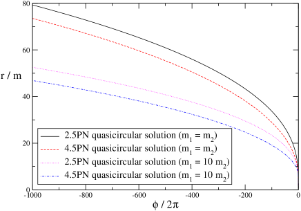
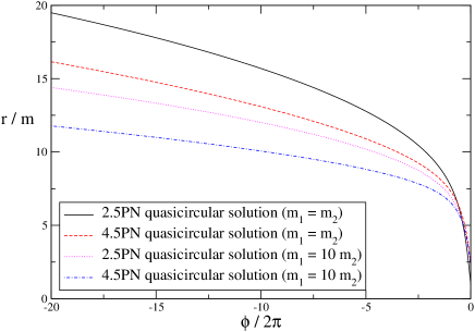
Figure 1: The orbital separation $r$ as a function of the number of orbits for the quasicircular solution of the 2.5PN and 4.5PN equations of motion. We show the equal mass ($m_{1}=m_{2}$) case along with the case of mass ratio $m_{1}/m_{2}=10$. The top panel displays the last 1000 orbits, the bottom panel displays the last 20 orbits.

As shown in Lincoln and Will (1990), the effect of the radiation reaction terms in the post-Newtonian equations of motion for highly separated compact binaries $(r>1000\>m)$ is to circularize the orbit of the binary. We refer to this state, and its subsequent solution to the post-Newtonian equations of motion as the unique (up to rotations) “quasicircular” solution. For an arbitrary binary separation $r_{i}$, initial data which corresponds to this quasicircular orbit scenario is given at 2PN order (see Lincoln and Will (1990)) as $\dot{r}_{i}=0$ with the square of the initial angular velocity $\dot{\phi}_{i}$ satisfying the cubic equation

$$0 = {(r_{i}^{2}\dot{\phi}_{i}^{2})}^{3}-\frac{m}{r_{i}}{(r_{i}^{2}\dot{\phi}_{i}^{2})}^{2}+(3-\eta){(\frac{m}{r_{i}})}^{3}{(r_{i}^{2}\dot{\phi}_{i}^{2})}-$$ (2)

$$(15+\frac{17}{4}\eta+2\eta^{2}){(\frac{m}{r_{i}})}^{5}.$$

Since this initial data does not give a true quasicircular evolution when considering equations of motion of order 2.5PN or higher, we use it as initial data for numerical integrations starting with large initial separations $r_{i}$ (typically $r_{i}>100\>m$), and allow the equations of motion to fully circularize the orbit, after which we refer to the solution as the unique (up to spatial rotations) quasicircular solution.

In Fig. 1, we plot the binary separation $r$ as a function of $\phi$ for the quasicircular solution to the 2.5PN and 4.5PN equations of motion for both the equal mass ($m_{1}=m_{2}$) case, as well as the case where the mass ratio $m_{1}/m_{2}$ is $10$. We easily use enough resolution so that the truncation error, if plotted as error bars on all curves in this paper, would be smaller than the thickness of the curves. We see that the 4.5PN solution displays a somewhat weaker radiation damping than the 2.5PN solution, in the sense that if one starts from a specific initial separation, there are more orbits until plunge for the 4.5PN solution as compared to the 2.5PN solution. For example, the bottom panel of Fig. 1 shows that for a circularized binary with orbital separation $r=15\>m$, the 2.5PN solution evolves for approximately 9 orbits until plunge (which, for definiteness, we define here as $r=2\>m$), whereas the 4.5PN quasicircular solution evolves for approximately 16 orbits until plunge. In Fig. 2, the ratio of the radial velocity $|\dot{r}|$ to the tangential velocity $r\dot{\phi}$ as a function of separation $r$ for the 2.5PN and 4.5PN quasicircular solutions is plotted, again for both the equal mass case and the mass ratio $m_{1}/m_{2}=10$ case. In both cases, we see that for separations $r>4\>m$, the ratio of the radial velocity to the tangential velocity is smaller for the 4.5PN solution than for the 2.5PN solution; once the separation reaches $4\>m$, the merger is a fraction of an orbit away for both the 2.5PN and 4.5PN solutions.

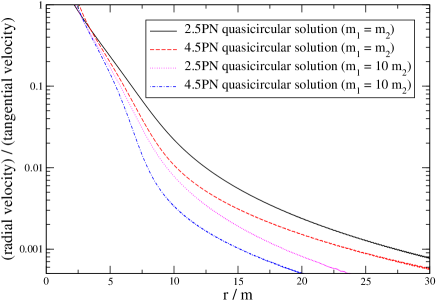
Figure 2: The ratio of the radial velocity $|\dot{r}|$ to the tangential velocity $r\dot{\phi}$ is plotted as a function of the binary separation $r$ for the quasicircular solution for both the 2.5PN equation of motion and the 4.5PN equation of motion. We show the equal mass ($m_{1}=m_{2}$) case along with the mass ratio $m_{1}/m_{2}=10$ case.

III Circular Initial Data and Subsequent Binary Evolution

The particular aspect of the quasiequilibrium approximation used in constructing initial data for binary systems of compact objects in numerical relativity that we analyze here is the circular orbit assumption. In practice, this assumption can take the form of an assumption of the existence of a helical Killing vector field; alternatively, turning point methods can be used to find approximate circular orbit configurations. The assumption of a circular orbit configuration as initial data in general relativity, while fully consistent from a mathematical point of view, is certainly questionable from an astrophysical point of view. A casual inspection of Figs. 1 and 2 reveals that a circular orbit assumption in the initial data for a realistic binary system (which we effectively define as a fully circularized binary; we ignore here any capture scenarios and/or dynamically driven scenarios where the binary could have high eccentricities all the way down to the plunge phase) will be increasingly inaccurate as the initial separation decreases. We note that considerations of computational resources alone will limit accurate simulations performed by numerical relativity codes in the coming decades to timescales of roughly $10$ orbital periods. From Fig. 1, this translates to initial binary separations $r_{i}<20\>m$. The relevant question is therefore: at what initial orbital separation $r_{i}$ does the circular orbit approximation break down? In other words, will gravitational waveforms produced from an evolution code using initial data corresponding to compact objects in exactly circular orbit be, in some sense, close enough to waveforms produced from the more astrophysically relevant quasicircular case? Here, we answer this question quantitatively using the PN approximation described in the previous section.

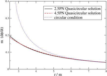
Figure 3: The angular velocity $\dot{\phi}=d{\phi}/dt$ is plotted as a function of binary separation $r$ for the quasicircular solution to the 2.5PN and 4.5PN equations of motion. Also shown is the angular velocity corresponding to instantaneously circular orbits ($\dot{r}=0$ and $\ddot{r}=0$, see Eq. 4) at separation $r$.

For an arbitrary initial separation $r_{i}$, we construct initial data at time $t_{i}=0$ corresponding to exact circular orbits by requiring the vanishing of the first and second time derivatives of the separation, $\dot{r}_{i}\equiv(dr/dt)|_{t=0}$ and $\ddot{r}_{i}\equiv(d^{2}r/dt^{2})|_{t=0}$. Assuming $\dot{r}_{i}=0$, the expression for the instantaneous radial acceleration $\ddot{r}_{i}$ is given by the equations of motion, Eq. 1, as

$$\ddot{r}_{i}=r_{i}{\dot{\phi}_{i}}^{2}+\frac{m}{r_{i}^{2}}(-1+A_{1PN}+A_{2PN}+A_{3PN}+\cdots).$$ (3)

We note that the radiation reaction terms (the n.5PN terms) do not enter in the prescription for circular data in the post-Newtonian approximation. Using the completely determined post-Newtonian $A_{1PN}$ and $A_{2PN}$ terms (see, e.g., Pati and Will (2002)), the expression for the instantaneous radial acceleration, Eq. 3, can be written explicitly as

$$\ddot{r}_{i} =r_{i}{\dot{\phi}_{i}}^{2}+\frac{m}{r_{i}^{2}}\left[\right. -1-(1+3\eta)r_{i}^{2}{\dot{\phi}_{i}}^{2}+2(2+\eta)\frac{m}{r_{i}}-$$ (4)

$$\eta(3-4\eta)r_{i}^{4}{\dot{\phi}_{i}}^{4}+\frac{1}{2}\eta(13-4\eta)mr_{i}{\dot{\phi}_{i}}^{2}-$$

$$\frac{3}{4}(12+29\eta){(\frac{m}{r_{i}})}^{2}.$$

We see that, to 2PN order, the equation $\ddot{r}_{i}=0$ (assuming $\dot{r}_{i}$ is also zero) becomes a quadratic equation for the square of the initial angular velocity $\dot{\phi}_{i}$. The initial circular orbit assumption, $\dot{r}_{i}=0$ and $\ddot{r}_{i}=0$, thus completely specifies the initial configuration for any arbitrary initial separation $r_{i}$. The initial angular velocity $\dot{\phi}_{i}$ for this circular condition is plotted in Fig. 3 as a function of initial separation $r_{i}$ for the equal mass binary case. For comparison, the angular velocity for the 2.5PN and 4.5PN quasicircular solution is also shown. We see that the circular orbit approximation induces an artificial increase in the angular velocity as compared to the more astrophysically relevant quasicircular solutions. Differences between the two become apparent at roughly $r=6\>m$, and by $r=3\>m$ the angular velocity for the circular orbit approximation is double that of the quasicircular solutions.

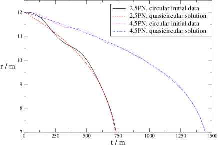
Figure 4: The evolved binary separation $r$ as a function of time $t$ is plotted for evolutions starting with circular initial data, with the initial separation $r_{i}=12\>m$ for the equal mass case ($m_{1}=m_{2}$). Both 2.5PN solutions and 4.5PN solutions are plotted. For comparison, the quasicircular solution is also shown for both the 2.5PN and 4.5PN case.

In Fig. 4, we plot solutions to the 2.5PN and 4.5PN equations of motion, using the initially circular conditions $\dot{r}_{i}=0$ and $\ddot{r}_{i}=0$ as initial data, with the initial separation $r_{i}=12\>m$. Here, we show the equal mass case, $m_{1}=m_{2}$. For comparison, the quasicircular solutions to the 2.5PN and 4.5PN equations of motion, where we have set $t=0$ when $r=12\>m$, are also shown. We see that the circular orbit approximation in the initial data induces oscillations (with a period of roughly $380\>m$) in the separation $r$, but that the evolutionary track of the two evolutions are similar. We see that for both the 2.5PN and 4.5PN circular initial data cases, the orbit is slightly eccentric, with $t=0$ corresponding to an apastron point in the orbit. Similar surveys of solutions starting with different initial binary separation parameter $r_{i}$ reveal the expected result that the oscillations in the evolved separation $r$ using circular initial data decrease monotonically as the initial separation $r_{i}$ increases; i.e., the “error” induced by assuming circular initial data decreases with increasing initial binary separation $r_{i}$. The fact that the circular orbit approximation induces an eccentricity in the orbit is not unexpected. It was shown in Mora and Will (2002) that allowing for eccentric orbits provided a better match between post-Newtonian turning point calculation results and numerical relativity turning point calculation results.

In order to get an idea of the phase errors induced by the circular orbit approximation, we calculate $\Delta\theta$, defined by

$$\Delta\theta=\sqrt{\frac{\int^{t_{f}}_{0}dt\>{(\theta_{c}(t)-\theta_{qc}(t))}^{2}}{t_{f}}},$$ (5)

which is a measure of the time averaged phase difference between the two solutions to the post-Newtonian equations of motion; $\theta_{c}(t)$ corresponding to the phase angle of the solution using circular orbit initial data and $\theta_{qc}(t)$ corresponding to the phase angle of the quasicircular solution, where each solution has an initial separation $r_{i}$ ($\Delta\theta$ is therefore an implicit function of initial separation $r_{i}$). Here, we introduce a cutoff time $t_{f}$, which we choose to be the time when either of the solutions reaches a binary separation of $r=3\>m$, since finite size effects become important for separations smaller than $r=3\>m$ for black holes (recall that in harmonic coordinates, the horizon of a static non-rotating black hole is located at $r=M$, where M is the mass of the black hole). In Fig. 5, we plot $\Delta\theta$ as a function of initial binary separation $r_{i}$ in the equal mass black hole case for both the 2.5PN and 4.5PN solutions. We see that a maximum is reached for initial binary separations of $r_{i}=8.8\>m$ and $r_{i}=8.1\>m$ for the 2.5PN and 4.5PN solutions, respectively. These separations correspond to roughly $1.5$ orbital periods before the final plunge.

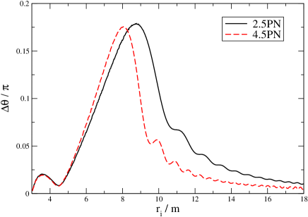
Figure 5: The time averaged phase difference, $\Delta\theta$ (Eq. 5), between the quasicircular solution and the solution using instantaneously circular initial data for evolutions starting with initial binary separation $r_{i}$. The solid curve corresponds to solutions to the 2.5PN equations of motion and the dashed curve corresponds to solutions to the 4.5PN equations of motion.

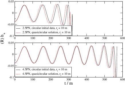
Figure 6: The “plus” (+) polarization gravitational waveform for coalescing, equal mass binaries. The top panel shows the radiation from solutions of the 2.5PN equations of motion and the bottom panel shows the radiation from solutions of the 4.5PN equations of motion. Both panels show the waveform for the solution starting with circular initial data and the quasicircular solution. The initial separation in each case is $r_{i}=10\>m$. The observation direction is in the orbital plane, with $\Theta=\pi/2$ and $\Phi=0$.

From a gravitational wave detection point of view, the relevant measure of how “close” the solutions starting with circular initial data are to the more astrophysically realistic quasicircular solutions is determined by examining the gravitational wave signal associated with each solution. We use the post-Newtonian formalism presented in Epstein and Wagoner (1975); Wagoner and Will (1976); Turner and Will (1978); Lincoln and Will (1990), which give the two polarization states $h_{+}$ and $h_{\times}$ for our solutions as a function of observer distance $R$ and observation directions $\Theta$ and $\Phi$. In Fig. 6, we show gravitational waveforms for solutions to the post-Newtonian equations of motion using initial data starting at $r_{i}=10\>m$. We see explicitly that the 2.5PN solution plunges within approximately two orbits, while the 4.5PN solution plunges within approximately four orbits (one orbital period is twice the period of the waveform). We also see that the phase of the waveform corresponding to the circular initial data slightly lags the phase of the more astrophysically realistic quasicircular solution in both the 2.5PN and 4.5PN cases. The effect is less pronounced in the 4.5PN case.

To quantify the difference between the gravitational waveform $h_{c}(t)$ obtained from circular initial data and the gravitational waveform $h_{qc}(t)$ obtained from the quasicircular solution, we define the correlation $C[h_{c}(t),h_{qc}(t)]$ of the waveforms as

$$C[h_{c}(t),h_{qc}(t)]=$$ (6)

$$\max_{\tau}\left\{\frac{\int^{t_{f}}_{0}h_{c}(t)h_{qc}(t-\tau)\>dt}{\sqrt{(\int^{t_{f}}_{0}{(h_{c}(t))}^{2}\>dt)(\int^{t_{f}}_{0}{(h_{qc}(t-\tau))}^{2}\>dt)}}\right\}.$$

Notice that the quantity inside the braces in the definition of the correlation $C[h_{c}(t),h_{qc}(t)]$ depends on both the lag time $\tau$ and the cutoff time $t_{f}$ for the time integrations. In our case, we specify the cutoff time $t_{f}$ as the earliest time when either of the waveforms corresponds to some “final” binary separation $r_{f}$. For black hole binaries, we expect tidal effects to become important as $r<3\>m$, so we set $r_{f}=3\>m$. For neutron star equal mass binaries, hydrodynamical effects will become important (depending on details of the equation of state) at around $r=9\>m$, in which case we set $r_{f}=9\>m$. Once the cutoff time $t_{f}$ is determined, the quantity inside the braces in Eq. 6 is a function of the lag time $\tau$; the final correlation $C[h_{c}(t),h_{qc}(t)]$ is determined by varying the lag time $\tau$ and finding the maximum value of the expression in braces. It is important to note that by introducing a cutoff of the gravitational waveform (which is necessary in a practical sense, due to the fact that the post-Newtonian approximation we are using breaks down when tidal effects become important), we are computing a lower bound of the error induced by using circular initial data for inspiral simulations; a more realistic calculation of the error would include all of the nonlinear phenomena occurring after tidal effects become important, which we are necessarily neglecting.

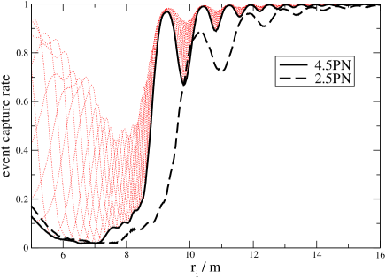
Figure 7: The event capture rate, $C[h_{c}(t),h_{qc}(t)]^{3}$ (where $C[h_{c}(t),h_{qc}(t)]$ is defined in Eq. 6), of 4.5PN gravitational waveforms using circular initial data as a function of initial binary separation $r_{i}$. The gravitational waveform observer is located in the orbital plane $\Theta=\pi/2$, with observer polar angles $\Phi=0$, $\pi/8$, $2\pi/8$, $3\pi/8$, $4\pi/8$, $5\pi/8$, $6\pi/8$, and $7\pi/8$ shown as thin dotted curves. The thick solid curve labeled “4.5PN” is the minimum correlation for all observation polar angles $\Phi$. This same minimum is plotted for the 2.5PN case and is labeled “2.5PN”.

In Fig. 7, we plot the cube of the correlation function $C[h_{c}(t),h_{qc}(t)]$, Eq. 6, between the waveform computed using circular initial data and the waveform of the quasicircular solution as a function of initial binary separation $r_{i}$, where we have set $r_{f}=3\>m$. This gives us an estimate of the lower bound of the event loss rate induced by using circular initial data instead of the more astrophysically correct quasicircular initial data in the case where the compact objects are black holes. For each initial separation $r_{i}$, we can find the minimum of the correlation over all observation polar angles $\Phi$, and take this to be the measure of the lower bound of the error induced by the circular orbit approximation in the initial data. This curve is labeled “4.5PN” in Fig. 7. The oscillations in this curve, which have a period of slightly more than one additional orbit in the evolution of the binary, correspond precisely to additional oscillations in the $r$ vs. $t$ curves (see Fig. 4). That is, as the initial binary separation $r_{i}$ increases, more oscillations in the $r$ vs. $t$ curve are allowed before the binary plunges, and the oscillations in Fig. 7 occur as a result. These oscillations are also evident in the time averaged phase difference, $\Delta\theta$ (Fig. 5), and occur for the same reason.

We see from Fig. 7 that, for any given initial separation $r_{i}$, the correlation between the waveform obtained from circular initial data and the waveform obtained from the quasicircular solution is larger for the 4.5PN solutions than for the 2.5PN solutions. However, recall from Fig. 1 that, for a given initial separation $r_{i}$, there is quite a large difference in the number of orbits before final plunge between the 2.5PN case and the 4.5PN case. From the standpoint of numerical relativity, the number of orbits before plunge is perhaps the more important criterion in parameterizing the orbital separation of the binary. In Fig. 8, we recast the results in Fig. 7, plotting the cube of the correlation function $C[h_{c}(t),h_{qc}(t)]$, Eq. 6, between the waveform computed using circular initial data and the waveform of the quasicircular solution as a function of the number of orbits until final plunge. We see that the profile of this event capture rate is similar for both the 2.5PN and 4.5PN cases, the major difference between the two being the phase of the oscillations. This gives us confidence that the post-Newtonian approximation has converged sufficiently to provide us with an accurate estimate of the lower bound of the error induced by the circular orbit assumption in the construction of initial data. The results of Figs. 7 and 8 are summarized in tabular form in Table 1. We can see that using circular initial data with configurations that have $2$ orbits until plunge or less will result in a $50\%$ or more event loss rate, and that one must start with configurations of $r_{i}>10\>m$ (with more than $3.5$ orbits until plunge) in order to have a chance of bounding the event loss rate to below $20\%$.

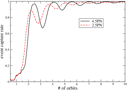
Figure 8: The event capture rate, $C[h_{c}(t),h_{qc}(t)]^{3}$ (where $C[h_{c}(t),h_{qc}(t)]$ is defined in Eq. 6), of gravitational waveforms from inspiraling black holes ($r_{f}=3\>m$) using circular initial data as a function of the number of orbits until plunge (i.e., until $r=2\>m$). The observer is located in the orbital plane $\Theta=\pi/2$, and the event capture rate is minimized over all polar angles $\Phi$ (see, e.g., Fig. 7). Results using both the 4.5PN and 2.5PN equations of motion are shown.

Event loss rate	minimum initial	minimum initial
	separation $r_{i}$ (2.5PN)	separation $r_{i}$ (4.5PN)
1%	$15.7\>m$ [9.8 orbits]	$13.8\>m$ [11.9 orbits]
5%	$12.7\>m$ [4.7 orbits]	$11.6\>m$ [6.3 orbits]
20%	$11.3\>m$ [3.1 orbits]	$10.0\>m$ [3.5 orbits]
50%	$9.6\>m$ [1.7 orbits]	$8.8\>m$ [1.9 orbits]
80%	$9.2\>m$ [1.5 orbits]	$8.6\>m$ [1.7 orbits]

Table 1: The minimum initial binary separation $r_{i}$ for specific event loss rates due to errors in the initial data introduced by the circular orbit approximation for black holes ($r_{f}=3\>m$), as predicted by the 2.5PN and 4.5PN equations of motion. In brackets are the number of orbits remaining until plunge, starting at this initial binary separation (see Figs. 7 and 8).

For neutron stars, we expect tidal effects to become important at binary separations $r$ of between $7\>m$ and $9\>m$, depending on the equation of state of the nuclear matter. As a result, the point particle approximation breaks down much earlier for neutron star models than for black hole models. This will necessarily result in a corresponding decrease in sensitivity when determining the errors induced by using circular orbit initial data. However, this does not necessarily imply that the errors induced by assuming initially circular orbits is less for neutron star binaries than those for black hole binaries at similar separations, but instead is simply an artifact that this particular model (spinless point particle model) is worse for neutron star binaries than for black hole binaries; after all, we are only computing lower bounds to these errors.

In Fig. 9, we set the cutoff separation $r_{f}$ to $9\>m$ (i.e., assuming neutron star binaries) and plot the cube of the correlation function $C$, Eq. 6, between the waveform computed using circular initial data and the waveform of the quasicircular solution as a function of initial binary separation $r_{i}$. As expected, we observe a notable decrease in sensitivity to errors induced by assuming initially circular data as compared to the black hole case ($r_{f}=3\>m$, see Figs. 7 and 8). In the case of equal mass binary neutron stars, the lower bound on the event loss rate that we compute is lower than $2\%$.

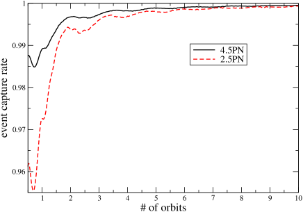
Figure 9: The event capture rate, $C[h_{c}(t),h_{qc}(t)]^{3}$ (where $C[h_{c}(t),h_{qc}(t)]$ is defined in Eq. 6), of gravitational waveforms from inspiraling neutron stars ($r_{f}=9\>m$) using circular initial data as a function of the number of orbits until separation $r=r_{f}=9\>m$, at which point hydrodynamical effects will become important. The observer is located in the orbital plane $\Theta=\pi/2$, and the event capture rate is minimized over all polar angles $\Phi$ (see, e.g., Fig. 7). Results using both the 4.5PN and 2.5PN equations of motion are shown.

IV Circular Initial Data: Comparing Post-Newtonian and Full Numerical Relativity Calculations

Numerical relativity has progressed to the point where stable, multiple orbit numerical simulations of compact objects are now possible. In Miller and Suen (2003), we present fully general relativistic simulations of binary neutron stars using conformally flat, quasiequilibrium initial data corresponding to an equal mass, corotating binary. The construction of the initial data, in addition to being a solution of the constraint equations of general relativity, assumed the existence of a timelike helical Killing vector field. That is, the binary is assumed to be instantaneously in a circular orbit. We wish to compare the numerical relativity calculations obtained in Miller and Suen (2003) with the post-Newtonian formulation from the previous sections. One difficulty in performing any such comparison is due to the fact that each calculation was performed in different coordinate systems. The post-Newtonian calculations are performed in a harmonic gauge ($g^{\alpha\beta}{\Gamma^{\mu}}_{\alpha\beta}=0$), whereas numerical relativity simulations typically use a variety of other (both local and elliptic-type) gauge conditions to specify the coordinates. In particular, the relativistic calculations of binary neutron stars presented in Miller and Suen (2003) used a quasi-isotropic coordinate system; the initial spatial slice is conformally flat, but the subsequent evolution of the full Einstein field equations drives the 3-metric away from conformal flatness. Nevertheless, we can attempt a comparison between the harmonic coordinate post-Newtonian calculations with the quasi-isotropic coordinate numerical relativity calculation by using a simple coordinate transformation that takes the single, stationary, non-rotating black hole solution of the Einstein equations written in harmonic coordinates Cook and Scheel (1997) to the same solution written in isotropic coordinates. Let $(t_{har},r_{har})$ and $(t_{iso},r_{iso})$ be the (time,radial) coordinate pair for the harmonic and isotropic coordinatizations, respectively. They are related by

$$r_{har} = r_{iso}+\frac{m^{2}}{4r_{iso}}$$

$$t_{har} = t_{iso}+4m\ln{\left(\frac{2r_{iso}-m}{2r_{iso}+m}\right)}.$$ (7)

We use this relationship to map the harmonic coordinate separation of the post-Newtonian calculations done in harmonic coordinates to the isotropic separation of the fully general relativistic calculations in Miller and Suen (2003) done in (quasi-) isotropic coordinates.

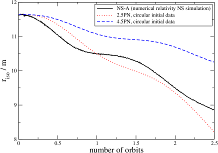
Figure 10: The isotropic separation of binary evolution calculations as a function of the number of orbits. Each calculation uses a circular orbit assumption as initial data. The solid curve refers to a fully consistent numerical relativity calculation of binary neutron stars using conformally flat, quasiequilibrium initial data (NS-A from reference Miller and Suen (2003)). The dotted and dashed curves correspond to 2.5PN and 4.5PN calculations, respectively, starting with the same initial isotropic separation as that of NS-A, assuming initially circular orbits.

In Fig. 10, we plot the isotropic, center of mass separation from the numerical relativity calculation NS-A of reference Miller and Suen (2003) as a function of the number of orbits. For comparison, we calculate the same quantity using the 2.5PN and 4.5PN equations of motion from the previous sections, starting with the same isotropic binary separation as that of NS-A and using the initially circular orbit assumption. The frequency of the oscillations in the separation is slightly different for the numerical relativity calculation NS-A as compared to the post-Newtonian calculations. There are many possible explanations for this. First of all, the calculations are done in different coordinate systems. While an attempt has been made to match the coordinates used to measure the binary separation (i.e., Eq. 7) in the two cases, the differences in the angular and/or time coordinates could explain the difference. Second, the numerical relativity calculation NS-A contains finite size effects, whereas the post-Newtonian approximation does not. Thirdly, the neutron stars in the initial data used for the NS-A numerical relativity calculation contain an unphysically high amount of spin, since the co-rotation assumption was used in its construction. The post-Newtonian approximation we are using does not take spin into account. Thus, any spin-orbit coupling in the NS-A calculation will not be present in the post-Newtonian approximation. Finally, the numerical errors in the calculation NS-A still could be large enough to explain the difference.

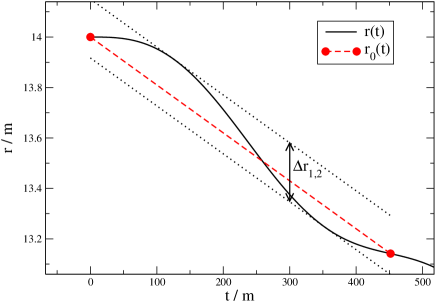
Figure 11: An example of the definition of ${\Delta r}_{1,2}$, used in the definition of the generalized eccentricity, Eq. 9. Here, $r(t)$ represents the 2.5PN solution using circular initial data at an initial binary separation of $r_{i}=14\>m$. The general apastron points are denoted by circles, and ${r_{0}}(t)$ is the line connecting the generalized apastron points.

However, the magnitudes of the oscillations in the separations shown in Fig. 10, which are a measure of the eccentricity of the orbits, are comparable. Notice that the separation $r$ is a monotonically decreasing function of time for all three calculations presented in Fig. 10. We note that this is universally true for post-Newtonian calculations using circular initial data. We therefore generalize the concept of an apastron point (typically defined as a local maximum of separation $r$) for monotonically decreasing binary separation functions r(t) as follows: if $r(t)$ is monotonically decreasing, then we define a generalized apastron point to be those points where $dr/dt$ attain a local maximum. We note that the numerical relativity calculation NS-A, as well as the 2.5PN and 4.5PN solutions using circular initial data, are initially ($t=0$ corresponds to $0$ orbits in Fig. 10) at generalized apastron points. Given any two consecutive generalized apastron points of a separation function $r(t)$ at, say, times $t_{1}$ and $t_{2}$, we can define the eccentricity $e_{1,2}$ as follows. Let ${\langle r\rangle}_{1,2}$ be the time averaged value of the binary separation $r$ between the two generalized apastron points:

$${\langle r\rangle}_{1,2}=\frac{\int^{t_{2}}_{t_{1}}dt\>r(t)}{(t_{2}-t_{1})}.$$ (8)

Let ${r_{0}}(t)$ be a linear function of time that intersects the points $r(t_{1})$ and $r(t_{2})$. We define ${\Delta r}_{1,2}$ to be the range of $r(t)-{r_{0}}(t)$ within the interval $t=[t_{1},t_{2}]$ (see Fig. 11). The generalized eccentricity $e$ is then defined as

$$e=\frac{{\Delta r}_{1,2}}{2\>{\langle r\rangle}_{1,2}}.$$ (9)

The advantages of this particular definition of the generalized eccentricity are twofold. In the first place, Eq. 9 reduces to the usual definition of eccentricity in the Newtonian limit. Secondly, it is defined in terms of quantities local to the binary, as opposed to quantities defined at spatial infinity. This makes it particularly useful in numerical relativity, where invariant measures of the binary separation can be straightforwardly computed.

In Fig. 12, we plot the generalized eccentricity $e$ (Eq. 9) for initially circular orbiting equal mass binaries as a function of initial binary separation $r_{i}$. The first generalized apastron point used in each calculation is at the initial time $t=0$. Shown are calculations using both the 2.5PN and 4.5PN equations of motion. At small values of initial separation $r_{i}$ (less than $r_{i}=10.07\>m$ for the 2.5PN equations of motion and $r_{i}=9.18\>m$ for the 4.5PN equations of motion) the solutions r(t) have monotonically decreasing first derivatives $dr/dt$, and thus do not exhibit multiple generalized apastron points (one could define the generalized apastron points in this case to be points where $d^{2}r/dt^{2}$ obtain local maxima, thereby further generalizing the definition of apastron points, but we have not done so here). For comparison, we show as a solid triangle in Fig. 12 the results from numerical relativity simulation NS-A from reference Miller and Suen (2003) of equal mass binary neutron stars using conformally flat, quasi-equilibrium initial data. In order to make the comparison more meaningful, we use Eq. 7 to relate the quasi-isotropic coordinate separation from the numerical relativity calculation to the harmonic coordinates used by the post-Newtonian calculation (although the difference between the two are quite small for $r_{i}=11.6\>m$). As can be seen, the eccentricity observed in the numerical relativity calculation NS-A lies between the 2.5PN and 4.5PN eccentricity predictions. Again, this comparison must be viewed as preliminary, as there still may exist significant numerical errors (i.e., boundary and/or truncation errors) in the numerical relativity simulations.

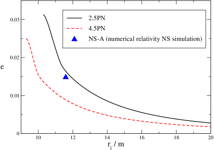
Figure 12: The generalized eccentricity $e$, Eq. 9, as a function of initial separation $r_{i}$ for initially circular orbiting equal mass binaries. Shown are results for both the 2.5PN and 4.5PN equations of motion. Also shown as the solid triangle is the eccentricity $e$ of the numerical relativity simulation of binary neutron stars NS-A from reference Miller and Suen (2003).

V Conclusions

In this paper, we have performed an analysis of the circular orbit approximation which is often used in the analysis of binary compact objects in general relativity. Using astrophysically relevant measures of the errors induced by the circular orbit approximation, we have shown that for equal mass binary black holes, the approximation has completely broken down for binary separations of $r\leq 8.5\>m$, which correspond to separations where roughly $2$ orbits or less remain before the final plunge. We conclude that numerical relativity evolution codes using circular orbit initial data configurations will be required to perform at least $3.5$ orbits (or more, depending on the accuracy required, see Table 1) in order to produce astrophysically meaningful waveforms to be used as search templates in modern interferometric gravitational wave detectors.

Finally, we comment on the astrophysical relevance of recent innermost circular orbit (ICO) calculations (for a review, see Baumgarte (2000); Blanchet (2002)). We note that all current calculations of ICO configurations for equal mass black holes have an angular velocity $m\dot{\phi}$ of as low as $0.06$ and as high as $0.18$. From Fig. 3, we see that this range corresponds to binary separations of $r=6\>m$ or less. Also, all current ICO calculations are based on the circular orbit approximation. However, we have shown in this paper that the circular orbit approximation has completely broken down for equal mass black holes with separations of $r\leq 8.5\>m$. This calls into question the astrophysical significance of ICO calculations based on circular orbit assumptions. Certainly, any gravitational waveforms produced from numerical relativity codes using initial data that corresponds to ICO configurations computed from circular orbit assumptions will be of little or no astrophysical significance.

VI Acknowledgement

It is a pleasure to thank Thierry Mora and Clifford Will for useful discussions and suggestions. Financial support for this research has been provided by the Jet Propulsion Laboratory (account 100581-A.C.02) under contract with the National Aeronautics and Space Administration. Computational resource support has been provided by the NSF NRAC project MCA02N022.

References

- Baumgarte et al. (1998a) T. W. Baumgarte, G. B. Cook, M. A. Scheel, S. L. Shapiro, and S. A. Teukolsky, Physical Review D 57, 7299 (1998a).
- Baumgarte et al. (1998b) T. W. Baumgarte, G. B. Cook, M. A. Scheel, S. L. Shapiro, and S. A. Teukolsky, Physical Review D 57, 6181 (1998b).
- Bonazzola et al. (1997) S. Bonazzola, E. Gourgoulhon, and J.-A. Marck, Phys. Rev. D 56, 7740 (1997).
- Gourgoulhon et al. (2001a) E. Gourgoulhon, P. Grandclement, K. Taniguchi, J. Marck, and S. Bonazzola, Phys. Rev. D 63, 064029 (2001a).
- Marronetti et al. (1999) P. Marronetti, G. J. Mathews, and J. R. Wilson, Phys. Rev. D60, 087301 (1999).
- Shibata (1998) M. Shibata, Phys. Rev. D 58, 024012 (1998).
- Teukolsky (1998) S. Teukolsky, ApJ 504, 442 (1998).
- Yo et al. (2001) H.-J. Yo, T. Baumgarte, and S. Shapiro, Phys. Rev. D 63 (2001).
- Duez et al. (2001) M. D. Duez, T. W. Baumgarte, and S. L. Shapiro, Phys. Rev. D63, 084030 (2001).
- Duez et al. (2002) M. D. Duez, T. W. Baumgarte, S. L. Shapiro, M. Shibata, and K. Uryu, Phys. Rev. D65, 024016 (2002).
- Gourgoulhon et al. (2001b) E. Gourgoulhon, P. Grandclement, and S. Bonazzola, Phys. Rev. D 65, 044020 (2001b).
- Grandclement et al. (2001) P. Grandclement, E. Gourgoulhon, and S. Bonazzola, Phys. Rev. D 65, 044021 (2001).
- Friedman et al. (2002) J. L. Friedman, K. Uryu, and M. Shibata, Phys. Rev. D 65, 064035 (2002).
- Cook (1994) G. B. Cook, Phys. Rev. D 50, 5025 (1994).
- Baumgarte (2000) T. W. Baumgarte, Phys. Rev. D 62, 024018 (2000).
- Blanchet et al. (1998) L. Blanchet, G. Faye, and B. Ponsot, Phys. Rev. D58, 124002 (1998).
- Itoh et al. (2001) Y. Itoh, T. Futamase, and H. Asada, Phys. Rev. D 63, 064038 (2001).
- Pati and Will (2002) M. E. Pati and C. M. Will, Phys. Rev. D 65, 104008 (2002).
- Damour et al. (2000) T. Damour, P. Jaranowski, and G. Schäfer, Phys. Rev. D 62, 021501 (2000).
- Blanchet and Faye (2001) L. Blanchet and G. Faye, Phys. Rev. D63, 062005 (2001).
- Gopakumar et al. (1997) A. Gopakumar, B. Iyer, and S. Iyer, Phys. Rev. D 55, 6030 (1997).
- Lincoln and Will (1990) C. W. Lincoln and C. M. Will, Phys. Rev. D 42, 1123 (1990).
- Mora and Will (2002) T. Mora and C. M. Will, Phys. Rev. D 66, 101501(R) (2002).
- Epstein and Wagoner (1975) R. Epstein and R. V. Wagoner, ApJ 197, 717 (1975).
- Wagoner and Will (1976) R. V. Wagoner and C. M. Will, ApJ 210, 764 (1976).
- Turner and Will (1978) M. Turner and C. M. Will, ApJ 220, 1107 (1978).
- Miller and Suen (2003) M. Miller and W.-M. Suen (2003), submitted.
- Cook and Scheel (1997) G. B. Cook and M. A. Scheel, Phys. Rev. D 56, 4775 (1997).
- Blanchet (2002) L. Blanchet, Phys. Rev. D65, 124009 (2002).