Toward standard testbeds for numerical relativity

Abstract

In recent years, many different numerical evolution schemes for Einstein’s equations have been proposed to address stability and accuracy problems that have plagued the numerical relativity community for decades. Some of these approaches have been tested on different spacetimes, and conclusions have been drawn based on these tests. However, differences in results originate from many sources, including not only formulations of the equations, but also gauges, boundary conditions, numerical methods, and so on. We propose to build up a suite of standardized testbeds for comparing approaches to the numerical evolution of Einstein’s equations that are designed to both probe their strengths and weaknesses and to separate out different effects, and their causes, seen in the results. We discuss general design principles of suitable testbeds, and we present an initial round of simple tests with periodic boundary conditions. This is a pivotal first step toward building a suite of testbeds to serve the numerical relativists and researchers from related fields who wish to assess the capabilities of numerical relativity codes. We present some examples of how these tests can be quite effective in revealing various limitations of different approaches, and illustrating their differences. The tests are presently limited to vacuum spacetimes, can be run on modest computational resources, and can be used with many different approaches used in the relativity community.

I Introduction

The inspiral of a relativistic binary has played the role of a standard candle for the first signal to be detected by the gravitational wave observatories which are now approaching operational readiness. For many years now, this has spurred activity to simulate the inspiral and merger of binary black holes using fully three-dimensional general relativistic evolution codes. Several groups across the world are dedicated to this endeavor but it still lies beyond present capability. The reasons for the difficulty of the binary black hole problem reflect the complexity of the underlying physics: the computational domain has a geometry whose metric is highly dynamic on vastly different time scales in the inner and outer regions, and it has a topology which is subject to change in order to avoid singularities. Even in the absence of black holes, there is no consensus on the best analytic and geometric formalism for dealing with the nonlinear nature of the gauge freedom and constraints of general relativity, and a numerical treatment greatly compounds the possibilities. The problem poses an enormous scientific challenge. See recent reviews such as Baumgarte and Shapiro (2003); Shinkai and Yoneda (2002a); Lehner (2001).

Substantial progress on small pieces of the problem has been made by individual groups but that progress is difficult to assess on a community level for the purpose of sharing ideas. A newcomer to the field would have to rely completely on anecdotal evidence in deciding how to develop a code. An observer or phenomenologist cannot judge the status of a code by wading through pages of Fortran and needs to view some standard tests to assess its reliability. Results are often published by various groups that report improvements in stability or accuracy in evolutions.; but formulations, gauges, numerical methods, boundary conditions and initial data can be inextricably mixed, and it is often difficult to sort out which ingredients in an improved treatment are crucial and against what standard the improvement is measured. Different groups invariably use different criteria for nearly all these issues. This paper is a first step toward remedying this situation by the establishment of standard testbeds that will help the numerical relativity community present and share results in an objective and useful way that will further scientific progress.

Apart from the practical aspects of providing a collection of standard tests as a community resource, the formulation of an appropriate test suite presents a significant scientific challenge. Comparing codes based upon different sets of variables with different sets of constraint equations is a nontrivial task. It is not straightforward to draw conclusions which would extend beyond the particular simulation for which the comparison was made. It is important to remain aware that evolution systems are a unity of evolution equations, boundary conditions and gauge. In order to paint a picture which gives heuristic insight into a broad panorama of “successes” and “failures”, it is essential to carefully design a set of tests involving different spacetimes and gauges. The current paper is a pivotal first step in this direction. Although it does not present a complete test suite, it provides some foundation for building one. We envisage the tests proposed here as the first round in a series of increasingly more complex tests.

In order to facilitate comparison of results, we will specify all tests as explicitly as possible. In addition to describing initial data and gauge, we will also specify a minimal set of output quantities, the setup of numerical grids, the choice of resolutions for convergence testing and even numerical methods. Although our choices aim at broad applicability, it is clear that they will not be optimal for many formulations. We foresee the usefulness of additional results, obtained with improved numerical methods or other modifications in the setup, which may promote further insight and clarification. We stress however, that results produced in a simple and identical numerical setup form the essential basis for a numerical comparison of different formulations of the equations. We present sample test results which illustrate and motivate such specifications. In this initial round of proposed tests, we also keep the spatial resolution rather low so as not to strain the computational resources of any group.

We believe that this project introduces a natural framework for documenting algorithms that “do not work”, which so far has been sorely lacking but is important for avoiding redundant experimentation. While failure in one particular case might be easy to detect, the general task of exploring and comparing different codes over a wide set of situations is complex.

Already nontrivial is the selection of criteria for comparison. Some standard criteria are:

1. Stability: Exponential growth (unless on a time scale significantly larger than the relevant physical timescale) is usually not tolerable in numerical simulations and should not occur if not inherent in the analytic problem.

2. Accuracy: Apart from resolution and numerical methods (which may be restricted by available computational resources), accuracy also depends on the analytic formulation.

3. Robustness: From a practical point of view, one is interested in a variety of physical situations. A robust code should be able to perform well in a wide class of spacetimes, gauges etc.

4. Efficiency: For 3D numerical relativity, time and memory constraints are severe. Thus computational efficiency is a serious issue.

5. Degree of mathematical understanding: Optimally one would like to mathematically demonstrate certain features of evolution systems, such as well-posedness or von Neumann stability.

In this work we focus on the issue of stability, and to some degree on accuracy. By devising a broad set of tests, we also shed some light on the question of robustness. At this stage, we do not investigate efficiency, i.e.  we do not consider our tests as benchmarks of computational performance regarding speed or memory requirements. Also, we adopt a practical, empirical point of view of what works and what does not, regardless of whether a mathematical theory is available. We hope, of course, that some of our results might stimulate theoretical progress. Indeed we hope that our work is not only useful for numerical relativists but also for a more general audience of relativists who are interested in the current state of numerical simulations. Furthermore, this work could be useful in facilitating communication between numerical relativists and the broad community of computational mathematicians and physicists.

The ideas presented here are an outgrowth of the “Apples with Apples” numerical relativity workshop held at UNAM in Mexico City during May 2002. The objective of the workshop was to formulate some basic tests that could be carried out by any group with a 3-dimensional code. What we report here are details of a selection of the first tests that were proposed and the principles that went into their design. The test results will be published at a later time. We encourage all groups, whether they attended the workshop or not, to contribute test results and share authorship in this second publication. While some tests may not be easily implemented in all formalisms, it is important for the calibration and support of progress in the field that the various groups submit as many test results as practical and conform as closely as possible to the test specifications. A web site www.ApplesWithApples.org has been set up to coordinate efforts and display results. Specific information about submitting tests results, and accessing results from other groups, can be obtained there. A continued series of workshops is being planned with the goal of developing increasingly more demanding tests leading up to black hole spacetimes with grid boundaries. The web site provides a forum for proposing new tests and coordinating plans for future workshops.

The round of preliminary tests presented here is of a simple nature designed to facilitate broad community participation. All tests use periodic boundary conditions, which is equivalent to evolution on the 3-torus in the absence of boundaries. Because the treatment of grid boundaries is one of the most serious open problems in numerical relativity, it is extremely useful to look in detail at this case which is not obscured by boundary effects. Only the Gowdy wave test is based on genuinely nonlinear data. The other tests involve weak and moderately nonlinear fields. Successful performance of an evolution code at this level is not obscured by either strong field effects or boundary effects and is indeed imperative for the successful simulation of black holes. The tests can be readily performed by any group with the capability of conducting fully 3-dimensional simulations. The value of this project depends critically on ease of implementation and flexibility of expansion to future tests.

The main purpose of the tests is to provide a framework for assessing the accuracy and long term stability of simulations based upon the wide variety of formulations and numerical approaches being pursued. All present codes are in a state of flux. The community needs clear information about “what works and what doesn’t” in order to carry out the continuous stream of modifications that must be made. This framework can be used to help compare the different ideas in meaningful ways; without standard points of reference it is nearly impossible to assess the effectiveness of one given approach relative to another.

As might be expected of a rapidly growing field, there is no established procedure for coordinating code tests with code development. In Section 2, we provide an overview of some of the current methodology being practiced to measure accuracy and stability. This provides the background for the discussion in Section 3 of our strategy in designing a series of code tests and comparisons which isolate in an effective way a set of performance levels necessary for successful simulation of black holes. In Section 4, we discuss the design specifications of the first round of tests, constructed so that code performance can be based on common output obtained from common input run on common grids. In Section 5 we summarize our work and discuss future perspectives. Our goal is to raise issues, collect ideas, point out pitfalls, document experiences and in general promote and stimulate work toward a better understanding of what works, what doesn’t and – ultimately – why.

We use the following conventions here: the spacetime metric has signature $(-,+,+,+)$; we use geometric units $G=c=1$; the Ricci tensor is $R_{ab}={R_{acb}}^{c}$; the extrinsic curvature is defined as $K_{ab}=-\frac{1}{2}{\cal L}_{n}h_{ab}$; where $h$ is the induced 3-metric and $n$ is the future directed timelike unit normal; this means that positive extrinsic curvature signifies collapse, and negative extrinsic curvature expansion.

II Current methodology

Test	Comments	Formulation	Reference
Slicings and perturbations	Harmonic gauge	ADM	Szilagyi and Winicour (2002)
of Minkowski space-time	Periodic gauge wave	KST / BM	Calabrese et al. (2002a, b); Bona and Palenzuela (2002)
	Periodic gauge wave with shift	ADM / BM	Bona et al. (1998)
	Gaussian gauge pulse	ADM / BM / BS	Balakrishna et al. (1996); Bona et al. (1998); Alcubierre et al. (2000a)
Hyperboloidal gauges	Compactifications of Minkowski	CFE	Hübner (1999); Husa (2002a)
	Radiation of Brill type	CFE	Husa (2002a)
	Weak data	CFE	Hübner (2001); Husa (2002b)
	Asymptotically A3	CFE, $\lambda$-CFE	Hübner (1999); Siebel and Hübner (2001)
Linearized solutions	Plane waves	ADM / BM	Bona et al. (1998); Anninos et al. (1997); Anninos et al. (1996a)
	Quadrupolar waves	ADM / BM	Bona et al. (1998); Allen et al. (1998a); Anninos et al. (1997)
	Teukolsky waves	ADM / BM / BSSN	Anninos et al. (1997); Anninos et al. (1996a); Abrahams et al. (1998); Baumgarte and Shapiro (1999)
	Scattering off Schwarzschild	ADM	Rezzolla et al. (1998)
	TT waves	SN	Shibata and Nakamura (1995)
Nonlinear plane waves	geodesic/densitized geodesic slicing	Ashtekar / $\lambda$-Ashtekar	Shinkai and Yoneda (2000); Yoneda and Shinkai (2001)
Gowdy Spacetimes	Expanding polarized	ADM	New et al. (1998)
	Collapsing polarized	ADM	Garfinkle (2002)
Robertson-Walker	$k=0$ (De Sitter)	BSSN	Vulcanov and Alcubierre (2001)
	$k=0$ (De Sitter) with cosmological constant	BSSN	Vulcanov and Alcubierre (2001)
Kasner		BSSN	Vulcanov and Alcubierre (2001)
Brill Waves	Maximal and 1+log slicing	BSSN	Alcubierre et al. (2000b)
Schwarzschild	Isotropic, geodesic slicing	ADM / BM	Bona et al. (1998); Brügmann (1996); Anninos et al. (1995a)
	Isotropic, algebraic slicing	ADM / BM	Bona et al. (1998); Arbona et al. (1999); Anninos et al. (1995a)
	Isotropic, maximal slicing	ADM / BM	Bona et al. (1998); Anninos et al. (1995a)
	Kerr-Schild (ingoing Eddington-Finkelstein)	adjADM/ KST / BSSN / LS / adjBSSN	Kelly et al. (2001); Kidder et al. (2001); Laguna and Shoemaker (2002); Alcubierre and Brügmann (2001); Yo et al. (2002)
	Painlevé-Gullstrand	adjADM / KST	Kelly et al. (2001); Kidder et al. (2001)
	Harmonic time slicing	KST	Kidder et al. (2001)
Distorted Schwarzschild		ADM / BM / BSSN	Camarda and Seidel (1998); Baker et al. (2000a); Allen et al. (1998a, b)
Kerr	Kerr-Schild	KST / adjBSSN	Kidder et al. (2001); Yo et al. (2002)
Distorted Kerr	algebraic slicing	BSSN	Alcubierre et al. (2003)
Misner Black Holes	Maximal slicing	ADM / BM / BSSN	Anninos et al. (1993); Anninos et al. (1995b, c, 1996b); Alcubierre et al. (2000b); Baker et al. (2000b)

Table 1: Solutions of the vacuum Einstein equations that have been used to validate Cauchy codes or formulations in the literature. The abbreviations of the formulations are following: ADM=Arnowitt-Deser-Misner Arnowitt et al. (1962); York (1979), adjADM=adjusted ADM Kelly et al. (2001); Shinkai and Yoneda (2002b), BM=Bona-Massó Bona et al. (1995), BSSN=Baumgarte-Shapiro-Shibata-Nakamura Baumgarte and Shapiro (1999), adjBSSN=adjusted BSSN Yoneda and Shinkai (2002), CFE=Conformal field eqs Friedrich (1981a, b), SN=Shibata-Nakamura Nakamura et al. (1987); Nakamura and Oohara (1989); Shibata and Nakamura (1995), KST=Kidder-Scheel-Teukolsky Kidder et al. (2001), LS=Laguna-Shoemaker Laguna and Shoemaker (2002), Ashtekar Yoneda and Shinkai (1999, 2000), and $\lambda$ = $\lambda$-system Brodbeck et al. (1999); Shinkai and Yoneda (1999).

As one of the primary aims of numerical relativity is to study spacetimes containing black holes, an important test of any code is its accuracy in simulating a black hole spacetime for which the solution is known analytically, such as Schwarzschild. However it is simpler to initially validate a code using spacetimes without singularities. This is illustrated by the list in Table 1 of some of the solutions previously used in the literature to validate 3+1 Cauchy vacuum codes. (A different set of testbeds has been used for characteristic codes Bishop et al. (1997); Husa et al. (2002).) The majority of tests have either used very weak field spacetimes, such as Minkowski space in various slicings or linearized waves, or used analytically known black hole spacetimes.

Most tests in Table 1 were developed for a particular application of a particular code. An attempt to define a general test suite for numerical relativity was considered quite early in Centrella et al. (1986). There the authors proposed 22 separate tests, 19 of which have an analytic solution (sometimes only in the Newtonian or linearized regime) or have quantities that can be calculated analytically. The emphasis in Centrella et al. (1986) is strongly toward relativistic hydrodynamics and only 5 of these tests can be applied to a vacuum code. These 5 tests focus on linearized and weak gravitational waves. The only strong field test is the simulation of a Brill wave, which does not have an analytic solution but if the amplitude is insufficient to form a black hole then the wave should disperse and the final radiated energy should equal the initial mass-energy.

Two points should be noted about the tests originally suggested in Centrella et al. (1986). First, none consider singularity formation or black holes. Since then, the binary black hole problem has become the primary focus of vacuum relativity codes and many subsequent tests have concentrated on single black holes, such as Schwarzschild (in various slicings) or Kerr. Perturbative solutions for distorted single black holes and their quasinormal modes also provide important checks. Second, all the tests in Centrella et al. (1986) were intended to test code accuracy. None of them was specifically intended to test stability. However stability has been the major problem for three dimensional relativity codes. Although the same analytic solutions could be used to study the stability of a code or of a formulation, the design of the test and the analysis of the results must be changed.

The standard approach in the field has not been to use a wide range of tests as suggested by Centrella et al. (1986). The tests in Table 1 were usually tailored to the specific problem of interest. For those papers interested in wave extraction, popular tests have included slicings of Minkowski, linearized and weak gravitational waves. Papers interested in black hole physics have used static or stationary black holes in various slicings. Evolutions of distorted black holes Camarda and Seidel (1998); Baker et al. (2000a); Allen et al. (1998a, b); Alcubierre et al. (2003) or colliding black holes Anninos et al. (1995c, 1996b); Alcubierre et al. (2000b); Baker et al. (2000b) have also been used to provide benchmarks for fully nonlinear codes. Papers investigating instabilities of various formulations or boundary conditions have tended to use slicings of Minkowski space Calabrese et al. (2002a), weakly constraint violating data Szilagyi et al. (2000); Szilagyi and Winicour (2002) or linearized waves, although black hole solutions have also been used Yo et al. (2002).

Many of these papers have concentrated on the convergence of the numerical code and have assumed that convergence is sufficient for a physically valid solution, even without a proof of the well-posedness of the continuum equations. The problems with this approach have been emphasized by various authors Calabrese et al. (2002a); Szilagyi et al. (2000); Szilagyi and Winicour (2002). Many formulations in use are either not well-posed or are not known to be well-posed with the gauge conditions or boundary conditions in practice. For example, many of the boundary conditions in use are inconsistent with the constraints and the evolution will converge to a valid solution only for the short time when it is causally disconnected from the boundary. As shown by Kreiss and Oliger Kreiss and Oliger (1973) and illustrated in the context of numerical relativity Calabrese et al. (2002a); Szilagyi et al. (2000), such gauge or boundary inconsistencies can lead to exponentially growing modes that may not appear in tests run at low resolutions or short time scales.

Choptuik Choptuik (1991); Cho (2002) has emphasized that if the continuum equations governing the evolution system and the constraints are well-posed and if the differencing scheme is consistent then some form of a Lax equivalence theorem should be expected to apply, i.e. that convergence and stability should be equivalent. Even in the absence of an exact solution, convergence can be checked in the Cauchy convergence sense by Richardson extrapolation and consistency can be checked by “independent residual evaluation” using an alternative discretization of the equations obtained by symbolic algebra techniques (see e.g. Miller (2000)). These methods give great confidence in the correctness of the numerical solution on the assumption that the underlying system of equations is well-posed. But that assumption lies beyond the analytic understanding of present day codes used to tackle the binary black hole problem.

III Design of standardized tests

Tests for numerical relativity should ideally satisfy a number of important properties. They should be broadly applicable, in the sense that they can be executed within a broad range of formulations. They should produce data which are unambiguous. They should specify free quantities such as the gauge. They should output variables which are independent of the details of the model and can be used for comparison. Finally, the tests and their output should provide some insight into both the characteristics of the code on which they are run and the comparative performance of other codes run on the same problem.

The first of these issues, universality, is not difficult to satisfy within a given class of codes. For instance, we can consider the class of “$3+1$” codes which evolve spacelike surfaces on a finite domain with periodic boundary conditions. For most formulations it should be a straightforward technical problem to express some initial data set in variables appropriate for a given formulation, and to construct the desired output variables at each time step. Even within this class of codes, however, details of implementation might restrict the set of tests which a particular code could run. For instance, codes which are fixed to run on a spherical domain might be difficult to test directly using data specified on a cube with periodic boundaries.

More serious difficulties arise in cross-comparing between classes of codes based upon entirely different formulations. Direct comparison of a finite domain code with a compactified characteristic code or with a Cauchy code based upon hyperboloidal time slices extending to null infinity would be impossible, given the difficulties in defining equivalent initial data. However, for a Cauchy code run on a large spatial domain, one could imagine comparing physically motivated quantities, such as the extracted radiation, with the results of a compactified code.

Of course, each test must specify an appropriate set of output quantities for analysis and comparison. It is common practice to judge the performance of a relativity code by measuring the degree of violation of the constraint equations. A properly working code should satisfy each of its constraints at each time-step. Constraint violation is a clear indication of a problem and usually the first indicator of growing modes which will eventually kill a simulation. On the other hand, a code which accurately preserves the constraints, perhaps by enforcing them during the evolution, might suffer other losses of accuracy which produce a numerically generated spacetime that is unphysical, even though it lies on the constraint hypersurface (for an example, see Siebel and Hübner (2001)). Solutions to the constraint equations are not necessarily connected via the evolution equations (e.g., a Schwarzschild spacetime should not evolve into Minkowski space, even though both will satisfy constraints perfectly!). Indeed, mixing constraint equations with the evolution equations can have great effect on the numerical results Yo et al. (2002). For these reasons, it is important not to examine the constraints in isolation. Similarly, the length of time a code runs before it “crashes” is not an appropriate criterion of quality unless accompanied by some indication of how accurately the code reproduces the intended physics, for example the constant amplitude and phase of a wave in the linear regime propagating inside a box with periodic boundaries.

Ideally, one would like to compare the convergence of variables against exact solutions where the answer is known. These are the most unambiguous tests and the most important for debugging a code. The exact solution provides an explicit choice of lapse and shift which can be adopted by any code through the use of gauge source functions. Furthermore, the exact solution provides explicit boundary data.

However, exact solutions for complex physical problems in relativity are scarce. We need additional criteria by which to judge whether numerically generated spacetimes are “correct”. For this one could include physical criteria, such as the energy balance between mass and radiation loss (for example, see Brandt and Seidel (1995); Alcubierre et al. (2001)). One could check some expected physical behavior of an evolution, such as the dispersion of a small amplitude Brill wave to evolve toward Minkowski spacetime, or the gravitational collapse of a high amplitude wave Alcubierre et al. (2000c). Unfortunately, such comparisons between codes can be misleading because of coordinate singularities produced by choice of gauge or by improper choice of boundary condition. For instance, the two spacetimes generated with the same initial data by two codes based upon harmonic time slicing might exhibit qualitatively different regularity properties because of different choices of shift. In such a case, the resulting difference in time slicings even complicates comparisons based upon curvature invariants because of the difficulty in identifying the same spacetime point in two different simulations. The same is true of spacetimes generated with the same initial data and gauge conditions but with different boundary conditions. Brill wave initial data which disperses to Minkowski space with a Sommerfeld boundary condition might collapse to a singularity with a Dirichlet boundary condition.

In the absence of exact solutions, convergence can be measured in the sense of Cauchy convergence. One might consider that a set of tests could be based upon the agreement between a number of independent convergent codes. However, caution needs to be taken with this approach since a common error could lead to acceptance of an incorrect numerical solution which then might systematically bias the modification of later codes to reproduce the accepted solution. Although convergence criteria are an important measure of the quality of any simulation, systematic problems can lead a code to converge to a physically irrelevant solution. Furthermore, agreement between codes is only straightforward when they use the same choice of lapse and shift, which is not always possible. Convergence tests should be accompanied by some expectation of how physical variables should behave. Initial data which have some physical interpretation, such as propagating waves, provide useful tests since they provide some picture of how the fields should behave. Any numerical relativity code should be able to reproduce such expected physical behavior if it is to be trusted when unexpected phenomena are encountered.

Ideally, tests should be “simple” as well as physical. For a simple enough test, some properties of a correct solution can be developed even if an exact solution is not known. Particular advantages and disadvantages of a code can be more readily isolated using simple tests for which the behavior of individual variables is understood. Of special importance, a simple test can be more readily implemented by a broad set of codes.

A characteristic feature of asymptotically flat systems is that energy gets lost through radiation. Correspondingly, the numerical treatment of such systems typically leads to an initial boundary value problem. However, in order to create a test suite which allows separation of problems associated with the boundary treatment from other problems, we believe it is fruitful to also consider tests with periodic boundaries. The use of periodic boundary conditions in testing numerical codes is a standard technique in computational science. In the context of general relativity, however, such tests have to be set up and interpreted with great care, since periodic boundaries create the cosmological context of a compact spatial manifold with the topology of a 3-torus. The resulting physics is qualitatively very different from asymptotically flat solutions. An example is the nonlinear stability of Minkowski spacetime, on which – at least implicitly – many numerical stability tests rely: For weak asymptotically flat data, it has been proved that perturbations decay to Minkowski spacetime Christodoulou and Klainerman (1993); Friedrich (1986). This result does not hold in the context of periodic boundaries! For two Killing vectors, it has been shown Andreasson et al. (2002) that all initial data which are not flat fall into two classes which are related to each other by time reversal. Making the standard cosmological choice of time direction, all non-flat data have a crushing singularity in the past and exist globally in a certain sense in the future. In particular, the spacetime can be covered by constant mean curvature hypersurfaces whose mean curvature goes to zero in the future Andreasson et al. (2002); Jurke (2003). In the simulation of such a spacetime, although the initial data analytically implies expansion, discretization error or constraint violation can drive the numerically perturbed spacetime toward a singularity in the future.

When $trK>0$ (in the present conventions) everywhere on a time slice, the pitfalls are easy to recognize. In that case, the singularity theorems (see e.g. Refs. Hawking and Ellis (1973) or Wald (1984)) imply that a singularity must form in finite proper time – even if the initial data are arbitrarily close to locally Minkowski data. Apart from such physical singularities, focusing effects can also create gauge singularities which could also lead to a code crash. Even in the $trK<0$ case where the spacetime undergoes infinite expansion, the code can crash due to choice of evolution variables that become infinite.

These observations introduce various complications for the setup and interpretation of numerical tests with periodic boundaries. For “linearized waves” with initial data close to Minkowski data, constraint violation or other source of error might lead to either expansion or collapse, with different codes exhibiting different behavior. For Minkowski data in nonstandard coordinates the situation is similar: Individual runs should be expected to show instabilities but with grid refinement the runs should show convergence to Minkowski spacetime. For situations with $trK>0$ on a whole time slice all codes should exhibit eventual collapse but in other cases the qualitative behavior may be code dependent. In order to interpret the results of a simulation it is thus vital to probe the underlying dynamics in terms of expansion versus collapse – in particular since many gauge conditions for the lapse involve $trK$. For this purpose, it is important to monitor such variables as $trK$, the eigenvalues of $K_{ab}$, $\det(g)$ and the total volume or proper time.

Since any given test will satisfy only a few of the desired criteria, some balance between redundancy and economy is needed. We can envisage a hierarchy of tests, starting from evolving flat space under various gauge assumptions, to linearized and then non-linear waves, to perturbations of a stationary black hole and then eventually to highly non-linear, dynamic black holes. Each successive test should introduce a new feature for which code performance can be isolated. The major goal of numerical relativity is the simulation of binary black holes. This requires special techniques, such as singularity excision, which by themselves are an extreme test for any code and can obscure the precise source of an instability arising in such a strong field regime. A standardized test suite should lead up to the binary problem through models of static, moving and perturbed black holes.

It is not our intention in this paper to present the specifics of a complete test suite. We concentrate here on an initial round of simple tests which serve to highlight certain important characteristics of the codes represented at the Mexico workshop and which can be readily performed with most codes. Even in trial implementations of these simple tests we have found complications that warn us that continuous feedback between design and experiment is absolutely necessary in developing a full test suite. The four tests in this initial round are: (i) the robust stability test, (ii) the gauge wave test, (iii) the linearized wave test and (iv) the Gowdy wave test.

Robust stability Szilagyi et al. (2000) is a particular good example of a testbed satisfying the above criteria. Random constraint violating initial data in the linearized regime is used to simulate unavoidable machine error. It can be universally applied, since any code can run perturbations of Minkowski space, and it is very efficient at revealing unstable modes, since at early times they are not hidden beneath a larger signal. Even in a convergence test based upon a non-singular solution, smoother truncation error dominates, at least until very late times, unless the resolution is very high. In stage I of the testbed, which we include in our first round of tests, evolution is carried out on a 3-torus (equivalent to periodic boundary conditions) in order to isolate problems which are independent of the boundary condition. In Stage II, one dimension of the 3-torus is opened up to form a 2-torus with plane boundaries, where random boundary data is applied at all times. This tests for stability in the presence of a smooth boundary. Boundary conditions which depend upon the direction of the outer normal, such as Neumann or Sommerfeld conditions, are best tested first with smooth boundaries in order to isolate problems. In Stage III, random data is applied at all faces of a cubic boundary, the common choice of outer boundary in simulating an isolated system. This tests for stability in the presence of edges and corners on the boundary. The test can be extended to Stage IV in which a spherical boundary is cut out of a Cartesian grid. These tests provide an efficient way to cull out unstable algorithms as a precursor to more time consuming convergence tests. The performance can be monitored by outputting the value of the Hamiltonian constraint.

The gauge wave testbed also very aptly fits our criteria. An exact wave-like solution is constructed by carrying out a coordinate transformation on Minkowski space. The solution can be carried out on a 3-torus, by matching the wavelength to the size of the evolution domain, or it can be carried out in the presence of boundaries. Since the gauge choice and boundary data are explicitly known, it is easy to carry out code comparisons. The evolution can be performed in the weak field regime or in the extreme strong field regime which borders on creating a coordinate singularity. Knowledge of a non-singular exact solution allows any instability to be attributed to code performance. Long, high resolution evolutions can be performed. Convergence criteria for the numerical solution can be easily incorporated into the test. In our first round of tests, we simulate a gauge wave of moderately non-linear amplitude propagating either parallel or diagonal to the generators of a 3-torus.

The linearized wave testbed uses a solution to the linearized Einstein equations and is complimentary to the first two. Run in the linearized regime, it provides an effectively exact solution of physical importance which can be used to check the amplitude and phase of a gravitational wave as it propagates on the 3-torus. If this test were run with a higher amplitude, so that nonlinear effects are not lost in machine noise, the constraint violation in the initial linearized data would introduce a complication. The tendency toward gravitational collapse could also amplify numerical error or the effect of a bad choice of gauge, e.g. the focusing effect inherent in Gaussian coordinates. A maximal slicing gauge cannot be used to avoid such problems, because, for any nontrivial solution, it would be inconsistent with periodic boundary conditions. While in the asymptotically flat context it is typical to use maximal initial hypersurfaces, it is known that a maximal Cauchy surface of $T^{3}$ topology has to correspond to locally Minkowski data (see e.g. Ref. Schoen and Yau (1979) and pages 2-3 of Ref. Anderson (2001)). This result is connected to the fact that $T^{3}$ does not admit metrics of positive Yamabe number, with the Yamabe number of flat $T^{3}$ being zero. In order to avoid these complications, our nonlinear wave tests, which complete the present round of testbeds, are based upon polarized Gowdy spacetimes. These spacetimes provide a family of exact solutions describing an expanding universe containing plane polarized gravitational waves Gowdy (1971) and a clear physical picture to test against the results of a simulation. We will carry out this test both in the expanding and collapsing time directions, which yields physically very different situations with potentially different mechanisms to trigger instabilities.

Except for the robust stability test, the remaining testbeds are based upon solutions with translational symmetry along one or two coordinate axes. By using the minimal required number of grid points along the symmetry axes, this allows the tests to be run with several grid sizes without exorbitant computational expense. Such tests could also be run with either 1D or 2D codes. In order to check that a 3D code is not taking undue advantage of the symmetry, the initial data can be superimposed with random noise as in the robust stability test. For purposes of economy we do not officially include this as part of the testbeds, but it is a useful practice which can completely alter the performance of a code.

IV test case specification

We will specify the physical properties of each testbed by providing the complete 4-metric of the spacetime, or if this is not possible, the initial Cauchy data and choice of gauge for the evolution. In all cases, we will give the Cauchy data, i.e. the 3-metric and extrinsic curvature, in a Cartesian coordinate system appropriate for 3-dimensional evolution. The physical domain is a cube which, in this first round of tests with periodic boundary conditions, represents a 3-torus.

In order for uniform comparison the series of four tests should be run using a second order iterative-Crank-Nicholson algorithm with two iterations (in the notation of Teukolsky (2000)) with second order accurate finite differencing in space. There may be codes that cannot implement this type of numerical method. Similarly, a particular code may run better with an alternative numerical method such as a Runge-Kutta time integrator or a pseudo-spectral method. In such cases the relative performance of the code for these tests still offers a useful comparison, provided all parameters (such as the amount of artificial dissipation) are held constant over the four tests. However, for a quantitative cross comparison of codes it is best to provide results from a standard numerical method. Second order iterative-Crank-Nicholson is chosen for simplicity.

The simulation domain for each test will generally be a cube of side $d$, equal to one wavelength with periodic boundary conditions. The grids are set up to extend an equal distance in the positive and negative directions along each axis. As depicted in Fig. 1, the “boundaries”, which are identified in the 3-torus picture, are located a half step from the first and last grid points along each axis. The resolution in a direction $i$ is given by $\Delta x^{i}=d/n^{i}$. The number of grid points $n^{i}$ should be sufficient to resolve features of the initial data in the given direction. Even though we are running three-dimensional codes, for tests with only one-dimensional features it is considerably more efficient to restrict the grid such that $n^{i}$ is small in the trivial directions. As an example, for a wave propagating in the $x$-direction we use the minimum number of grid points in the trivial $y$ and $z$ directions that allow for non-trivial numerical second derivatives. For standard second order finite differencing this implies that we use 3 points in those directions.

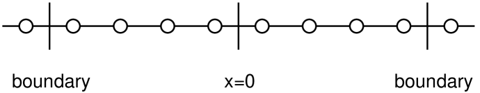
Figure 1: Grid points (in this case n=8) along a given axis are chosen to straddle both $x=0$ and the identified boundaries. An arbitrary number of ghost-zone points beyond the boundaries can be used in implementing periodic boundary conditions.

The size of the timestep $dt$ is given in terms of the grid size $dx$ and chosen to lie within the CFL limit for an explicit evolution algorithm. We foresee the possibility of codes for which this would be inappropriate and for which some equivalent choice of time step would have to be made. A final time $T$, and intermediate times for data output, are specified for each test. The time $T$ is chosen to incorporate all useful features of the test without prohibitive computational expense. The output times should be appropriately modified for codes that crash before time $T$.

The output quantities are chosen with either some physical or numerical motivation in mind. Both quantitative and qualitative comparisons are used. Some examples, based upon representative versions of evolution codes, are provided below for purposes of illustration. We specify a minimum list of output quantities. Other quantities that we do not include here but that may be of interest for a specific code include the Fourier transform of differences between the numerical and exact solutions as in Calabrese et al. (2002a), curvature invariants to detect deviations from flat space, and proper time integrated along observer world lines. Each group should of course also output any additional variables which are essential to the performance of their particular formulation.

IV.1 Robust stability testbed

The robust stability testbed Szilagyi et al. (2000) efficiently reveals exponentially growing modes which otherwise might be masked beneath a strong initial signal for a considerable evolution time. It is based upon small random perturbations of Minkowski space. The initial data consists of random numbers $\epsilon$ applied as a perturbation at each grid point to every code variable requiring initialization. For example, the initial 3-metric is initialized as $h_{ij}=\delta_{ij}+\epsilon_{ij}$, where the $\epsilon_{ij}$ are independent random numbers. The range of the random numbers ensures that $\epsilon^{2}$ effects are below roundoff accuracy so that the evolution remains in the linear domain unless instabilities arise.

For economy, we fix the following parameters:

• Simulation domain: $x\in[-0.5,+0.5]$

• Grid: $x_{n}=-0.5+(n-\frac{1}{2})dx,\quad n=1\ldots 50\rho,\quad dx=dy=dz=1/(50\rho),\quad\rho\in\mathbb{Z}$

• Time step: $dt=dx/2=0.01/\rho$

The parameter $\rho$ allows for refinement testing, which clarifies the results as can be seen in Figure 2. The values used in that test were $\rho=1,2,4$. We use the minimum number of grid points in the $y,z$ directions that allow for non-trivial numerical second derivatives – this means we carry out this test in a long channel rather than a cube. For standard second order finite differencing this implies that we use 3 points in the $y$ and $z$ directions.

The amplitude of the random noise should be scaled with the grid spacing as

$$\epsilon\in(-10^{-10}/\rho^{2},+10^{-10}/\rho^{2}).$$ (1)

This ensures that the norm of the Hamiltonian constraint violation in the initial data will be (on average) the same for different values of the refinement factor $\rho$. This means that in the continuum limit we will have a solution that is not a solution of the Einstein equations but “close” to one. This would be the case in a real numerical evolution where machine precision takes the place of $\epsilon$. If a code cannot stably evolve the random noise then it will be unable to evolve a real initial data set.

The test should be run for a time of $T=1000$ (corresponding to $1000$ crossing times) or until the code crashes. Performance is monitored by outputting the $L_{\infty}$ norm of the Hamiltonian constraint once per crossing time, i.e. at $t=0,1,2,3,...$. Because the initial data violates the constraints, any instability can be expected to lead to an exponential growth of the Hamiltonian unless enforcement of the Hamiltonian constraint were built into the evolution algorithm. As an example, Figure 2 shows the performance of standard ADM and BSSN codes and illustrates the efficacy of this test in revealing unstable codes.

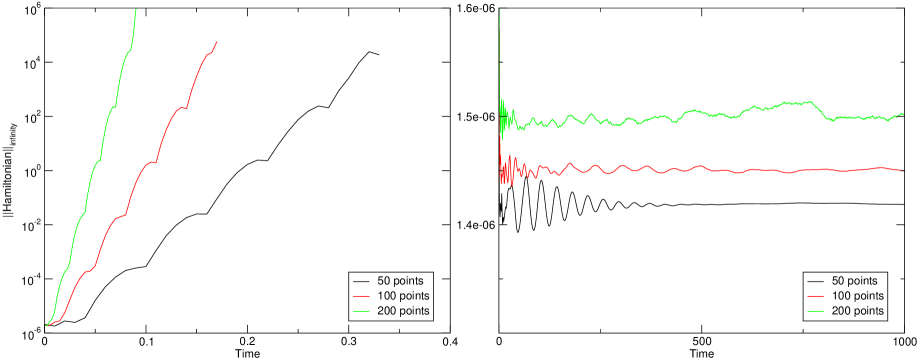
Figure 2: Left: the robust stability test applied to the standard formulation of the ADM equations. It is clear that there is an exponentially growing mode and that the growth rate of the mode depends on resolution. Right: the robust stability test applied to the BSSN formulation. The violation of the constraint is approximately constant even after 1000 crossing times. In both cases the harmonic gauge was used. Note the differences in the axes.

IV.2 Gauge wave testbed

These tests look at the ability of formulations to handle gauge dynamics. This is done by considering flat Minkowski space in a slicing where the 3-metric $h_{ij}$ is time dependent. Such gauge waves have been considered before, notably by Alcubierre (1997) and Calabrese et al. (2002a).

We have considered different profiles for gauge waves. For the purpose of this paper we focus on the case of a propagating gauge sine wave. This specific test was used in comparing systems with different hyperbolicity properties in Calabrese et al. (2002a).

The 4-metric is obtained from the Minkowski metric $ds^{2}=-d\hat{t}^{2}+d\hat{x}^{2}+d\hat{y}^{2}+d\hat{z}^{2}$ by the coordinate transformation

$$\begin{array}[c]{r c l}\hat{t}&=&t+\frac{Ad}{4\pi}\cos\left(\frac{2\pi(x-t)}{d}\right),\\ \hat{x}&=&x-\frac{Ad}{4\pi}\cos\left(\frac{2\pi(x-t)}{d}\right),\\ \hat{y}&=&y,\\ \hat{z}&=&z\end{array}$$ (2)

where $d$ is the size of the evolution domain. This leads to the 4-metric

$$ds^{2}=-Hdt^{2}+Hdx^{2}+dy^{2}+dz^{2},$$ (3)

where

$$H=H(x-t)=1+A\sin\left(\frac{2\pi(x-t)}{d}\right),$$ (4)

which describes a sinusoidal gauge wave of amplitude $A$ propagating along the $x$-axis. The extrinsic curvature is given by

$$K_{xx} = -\frac{\pi A}{d}\frac{\cos\left(\frac{2\pi(x-t)}{d}\right)}{\sqrt{1+A\sin\left(\frac{2\pi(x-t)}{d}\right)}},$$ (5)

$$K_{ij} = 0\qquad\textrm{ otherwise}.$$ (6)

Since this wave propagates along the $x$-axis and all derivatives are zero in the $y$ and $z$ directions, the problem is essentially one dimensional and can simplify the system dramatically for certain formulations, as there is no finite-difference error in the orthogonal directions. A simple coordinate transformation causes the wave to propagate along a diagonal:

$$x=\frac{1}{\sqrt{2}}(x^{\prime}-y^{\prime}),\qquad y=\frac{1}{\sqrt{2}}(x^{\prime}+y^{\prime})$$ (7)

The resulting metric is a function of

$$\sin\left(\frac{2\pi(x^{\prime}-y^{\prime}-t^{\prime}\sqrt{2})}{d^{\prime}}\right),\quad\textrm{where}\quad d^{\prime}=d\sqrt{2}\,.$$ (8)

Setting $d^{\prime}$ to the size of the evolution domain in the $x^{\prime}$ and $y^{\prime}$ directions gives periodicity along those directions. This test should be run in both axis-aligned and diagonal form.

As any evolution is a pure gauge effect, care must be taken in the choice of lapse and shift to allow a direct comparison between formulations. For example, the Bona-Masso family of gauges Bona et al. (1995)

$$\partial_{t}\alpha=-\alpha^{2}f(\alpha)K$$ (9)

will propagate a gauge wave in direction $x^{i}$ with speed $\alpha\sqrt{fg^{ii}}$, which can be varied. In contrast, maximal slicing would freeze any gauge pulse, stopping it from propagating.

Note that the time coordinate $t$ in the metric (3) is harmonic, which corresponds to

$$f(\alpha)=1.$$ (10)

This gauge condition can easily be integrated to $\alpha=h(x^{i})\sqrt{(}\det g)$. Also, in this case the gauge speed is simply the speed of light. To ensure that we can directly compare as many formulations as possible we choose harmonic slicing to carry out the evolution for the gauge wave test. Different formulations and codes may demand different implementations of harmonic time slicing for optimal performance. The test should thus be implemented in a way that is analytically compatible with the metric (3), which still leaves significant freedom.

We run the gauge wave with amplitudes $A=10^{-1}$ and $A=10^{-2}$. We have found that smaller amplitudes are quite simple for all codes whilst larger amplitudes can cause numerical error to trigger gauge pathologies, such as the formation of coordinate singularities, very quickly.

The specified wave has wavelength $d=1$ in the 1D simulation and wavelength $d^{\prime}=\sqrt{2}$ in the diagonal simulation. We find that 50 grid points are sufficient to resolve the profile and therefore make the following choices for the computational grid:

• Simulation domain:

  1D:	$\quad x\in[-0.5;+0.5],$	$\quad y=0,$	$\quad z=0,$	$\quad d=1$
  diagonal:	$\quad x\in[-0.5;+0.5],$	$\quad y\in[-0.5;+0.5],$	$\quad z=0,$	$\quad d^{\prime}=\sqrt{2}$

• Grid: $x^{i}=-0.5+(n-\frac{1}{2})dx,\quad n=1\ldots 50\rho,\quad dx=1/(50\rho),\quad\rho\in\mathbb{Z}$

• Time step: $dt=dx/4=0.005/\rho$

The 1D evolution is carried out for $T=1000$ crossing times, i.e. $2\times 10^{5}\rho$ time steps (or until the code crashes), with output every 10 crossing times. The 2D diagonal runs are carried out for $T=100$, with output every crossing time. We run using $\rho=1,2,4$.

We output the $L_{2}$, the maxima and minima, and profiles along the $x$-axis through the center of the grid of $g_{xx}$, $\alpha$, $tr(K)$, the Hamiltonian constraint and any other independent constraints that arise in a nontrivial way in a particular formulation. We also calculate the $L_{2}$-norm of the difference from the exact solution for $g_{xx}$ and calculate the convergence factor. Figure 3 provides examples of test output obtained with a standard ADM code. These results do not show a problem with ADM, but illustrate the expansion of the numerical space-time. This is due to the reasons mentioned in section III, stating that any non trivial space-time with $T^{3}$ topology must have a singularity either in the past or in the future. The behavior of the $L_{2}$-norm of $g_{xx}$ indicates how the volume element of the space behaves. It is also seen that the evolution is convergent for a long time, nevertheless the higher order terms cause the deviation from convergence.

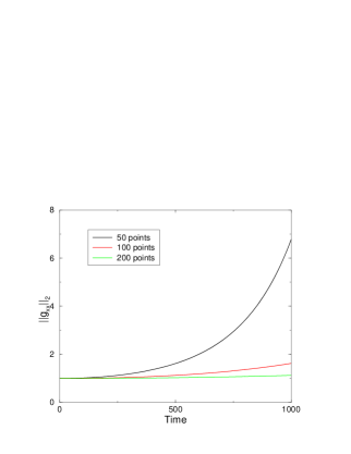
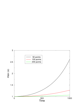
Figure 3: Results for the 1D gauge wave using the standard ADM formulation. The left hand plot shows $||g_{xx}||_{2}$; the central plot shows the maximum of the lapse $\alpha$, and the right hand plot shows the convergence factor of $g_{xx}$ calculated using the three resolutions. A value of $4$ would mark exact second order convergence.

IV.3 Linear wave testbed

This test checks the ability of a code to propagate the amplitude and phase of a traveling gravitational wave. The test is run in the linear regime where there are no complications due to the toroidal topology implicit in periodic boundary conditions. It reveals effects of numerical dissipation and other sources of inaccuracy in the evolution algorithm. We note that the evolution is meaningless once the accumulation of numerical error takes it out of the linear regime.

The initial 3-metric and extrinsic curvature $K_{ij}$ are given by a diagonal perturbation with components

$$ds^{2}=-dt^{2}+dx^{2}+(1+b)\,dy^{2}+(1-b)\,dz^{2},$$ (11)

where

$$b=A\sin\left(\frac{2\pi(x-t)}{d}\right)$$ (12)

for a linearized plane wave traveling in the $x$-direction. Here $d$ is the linear size of the propagation domain, and the metric is written here in Gauss coordinates, i.e. with lapse $\alpha=1$ and shift $\beta^{i}=0$. The nontrivial components of extrinsic curvature are then

$$K_{yy}=\frac{1}{2}\partial_{t}b,\quad K_{zz}=-\frac{1}{2}\partial_{t}b.$$ (13)

As in the case of the gauge wave, by the simple coordinate transformation

$$x=\frac{1}{\sqrt{2}}(y^{\prime}+x^{\prime}),\qquad y=\frac{1}{\sqrt{2}}(y^{\prime}-x^{\prime})$$ (14)

the propagation direction can be aligned with a diagonal. Setting $d^{\prime}=d\sqrt{2}$ to the size of the evolution domain in the $x^{\prime}$, $y^{\prime}$ directions gives periodicity along those directions.

The amplitude of the wave is chosen as $A=10^{-8}$, such that quadratic terms are of the order of numerical roundoff. Larger amplitudes mean that the solution does not stay in the linear regime sufficiently long.

The geometry of the grid is chosen identical to the 1D gauge wave test, with $d=1$ in the 1D case and $d^{\prime}=\sqrt{2}$ in the diagonal case:

• Simulation domain:

  1D:	$\quad x\in[-0.5;+0.5],$	$\quad y=0,$	$\quad z=0,$	$\quad d=1$
  diagonal:	$\quad x\in[-0.5;+0.5],$	$\quad y\in[-0.5;+0.5],$	$\quad z=0,$	$\quad d^{\prime}=\sqrt{2}$

• Grid: $x^{i}=-0.5+(n-\frac{1}{2})dx,\quad n=1\ldots 50\rho,\quad dx=1/(50\rho),\quad\rho\in\mathbb{Z}$

• Time step: $dt=dx/4=0.005/\rho$

As in the gauge wave case, the 1D evolution is carried out for $T=1000$ crossing times, i.e. $2\times 10^{5}\rho$ time steps (or until the code crashes), with output every 10 crossing times. The 2D diagonal runs are carried out for $T=100$, with output every crossing time. For the trivial directions ($y$ and $z$ for the wave propagating along the $x$ axis and $z$ for the wave propagating along the diagonal) we use the minimum number of grid points in the $y,z$ directions that allow for non-trivial numerical second derivatives. For standard second order finite differencing this implies that we use 3 points in the appropriate directions. We run using $\rho=1,2,4$.

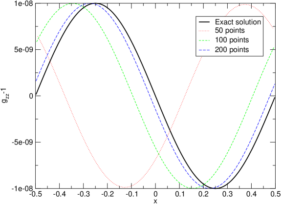
Figure 4: A 1D linear wave shown at different resolutions. Although the run lasted 1000 crossing times, the output is shown after 500 crossing times in order to indicate the trend of how resolution effects phase accuracy. The numerical dissipation is low but the cumulative phase error is high at the coarser resolutions. It is clear that the phase error converges away. The results are from the code ABIGEL which implements a fully harmonic formulation Szilagyi and Winicour (2002).

The output quantities are similar to those for the gauge wave: the $L_{\infty}$ and $L_{2}$-norms, the maxima and minima, and profiles along the $x$-axis through the center of the grid of $g_{yy}$, $g_{zz}$, $tr(K)$, the Hamiltonian and any other nontrivial constraints, and the $L_{\infty}$-norm of the difference from the linear exact solution for $g_{zz}$. Figure 4 illustrates the profiles of $g_{zz}-1$ obtained using a code based upon harmonic coordinates.

IV.4 Polarized Gowdy wave testbed

All of the tests described so far considered initial data which were perturbations of a flat background. Here we use a genuinely curved exact solution – a polarized Gowdy spacetime – to test codes in a strong field context. The polarized Gowdy $T^{3}$ spacetimes are solutions of the vacuum Einstein equations on the 3-torus, and describe an expanding universe containing plane polarized gravitational waves Gowdy (1971). Gowdy spacetimes have previously been used for testing numerical relativity codes by a number of authors van Putten (1997); New et al. (1998); Garfinkle (2002). They have also extensively been studied in mathematical cosmology; see e.g. Ringstrom (2003) for latest results. An extensive analytical and numerical study of Gowdy spacetimes has been carried out by Berger Berger (2002).

The polarized Gowdy metric is usually written as

$${ds}^{2}=t^{-1/2}e^{\lambda/2}(-{dt}^{2}+{dz}^{2})+t\,{dw}^{2},$$ (15)

where

$${dw}^{2}=e^{P}{dx}^{2}+e^{-P}{dy}^{2}.$$ (16)

Here the time coordinate $t$ is chosen such that time increases as the universe expands. For code testing, it is quite interesting to compare collapsing and expanding situations. We will thus carry out our tests in both time directions. The quantities $\lambda$ and $P$ are functions of $z$ and $t$ only and are periodic in $z$. The metric is singular at $t=0$ which corresponds to the cosmological singularity.

With the metric (15), the Einstein evolution equations can be reduced to a single linear equation for $P$ Gowdy (1971):

$$P_{,tt}+t^{-1}\,P_{,t}-P_{,zz}=0.$$ (17)

The constraint equations become

$$\lambda_{,t}=t\,(P_{,t}^{2}+P_{,z}^{2})$$ (18)

and

$$\lambda_{,z}=2\,t\,P_{,z}\,P_{,t},$$ (19)

and correspond to the Hamiltonian (18) and momentum (19) constraints. The general solution to eq. (17) is a sum of terms of the form $\alpha\log t+\beta$, where $\alpha$ and $\beta$ are real constants, and terms of the form $Z_{0}(2\pi nt)\cos(2\pi nz)$ and $Z_{0}(2\pi nt)\sin(2\pi nz)$, where $n$ is an integer (assuming periodicity of 1 in $z$) and $Z_{0}$ is a linear combination of the Bessel functions $J_{0}$ and $Y_{0}$. We follow New et al. (1998) in the choice of the particular solution and set

$$P=J_{0}(2\pi t)\cos(2\pi z),$$ (20)

which yields

$$g_{xx}=te^{P},\ g_{yy}=te^{-P},\ g_{zz}=t^{-1/2}e^{\lambda/2},$$ (21)

$$K_{xx} = -\frac{1}{2}t^{1/4}e^{-\lambda/4}e^{P}(1+tP_{,t}),$$

$$K_{yy} = -\frac{1}{2}t^{1/4}e^{-\lambda/4}e^{-P}(1-tP_{,t}),$$ (22)

$$K_{zz} = \frac{1}{4}t^{-1/4}e^{\lambda/4}(t^{-1}-\lambda_{,t}).$$

The shift vanishes, and the lapse is given as

$$\alpha=\sqrt{g_{zz}}=t^{-1/4}e^{\lambda/4}.$$ (23)

Using our choice for $P$ (20), the constraint eqs. (18,19) yield an expression for $\lambda$:

$$\begin{array}[c]{r c l}\lambda&=&-2\pi tJ_{0}(2\pi t)J_{1}(2\pi t)\cos^{2}(2\pi z)+2\pi^{2}t^{2}\bigl{[}J_{0}^{2}(2\pi t)+J_{1}^{2}(2\pi t)\bigr{]}\\ &&\mbox{}-{\frac{1}{2}}\bigl{\{}(2\pi)^{2}\bigl{[}J_{0}^{2}(2\pi)+J_{1}^{2}(2\pi)\bigr{]}-2\pi J_{0}(2\pi)J_{1}(2\pi)\bigr{\}}.\end{array}$$ (24)

Note that $A=\int_{z}tP_{,t}\,dz$ is a constant of motion and can be used to monitor the accuracy of a code. In our case $A$ is set to zero by the choice of initial data.

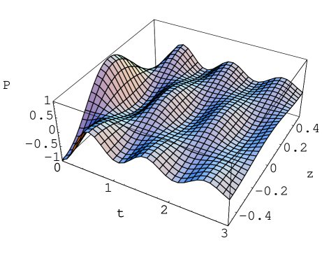
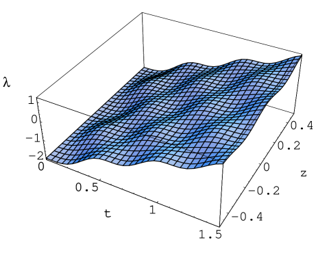
Figure 5: The quantities $P$ and $\lambda$ appearing in the Gowdy metric (15) are plotted versus $z$ and $t$.

Figure 6: The extrinsic curvature components $K_{xx}$ and $K_{zz}$, as given in Eqs. (22), and $trK$ at the coordinate origin are plotted versus time $t$.

Figures showing $P$, $\lambda$ and extrinsic curvature components, constructed from the analytic formulas, are given in Figures 5 and 6. While $P$ slowly decays to zero, $\lambda$ shows a secular linear growth due to the cosmological expansion, and both $P$ and $\lambda$ exhibit gravitational wave oscillations. Note that although the individual extrinsic curvature components do not exhibit a fixed sign, $trK$ is negative and decays in absolute value, consistent with the cosmological expansion. The linear growth of $\lambda$ leads to exponential growth in the metric component $g_{zz}$. This makes an evolution with standard $3+1$ ADM variables much harder than evolving the Gowdy quantity $P$.

The (coordinate) velocity of light is constant in the coordinates chosen in eq. (15), and with a fixed spatial discretization size $\Delta z$ the Courant condition is consistent with a fixed timestep $\Delta t$. This makes it convenient to choose the gauge (15) for evolving in the expanding direction. We will see below however, that this leads to exponential growth in the metric component $g_{zz}$. For the collapsing direction, this would lead to a singularity at $t=0$, so we will evolve this case with a different slicing as discussed below.

For the forward (expanding) evolution, we set initial data from the exact solution at $t=1$, which yields initial data of order unity, and evolve with any lapse condition which is equivalent in the continuum limit to the exact lapse given by eq. (23). Due to the exponential growth in the metric variables, such evolutions may crash rather soon but will test the accuracy of a code in a rather harsh situation. In order to evolve in the backward time direction, we choose harmonic time slicing, as has previously been done by Garfinkle Garfinkle (2002). Since harmonic slicing is marginally singularity avoiding Bona et al. (1997); Alcubierre (2003), such evolutions should only asymptotically reach the singularity at $t=-\infty$.

It turns out that it is actually quite simple to write down an exact solution for harmonic slicing, which greatly simplifies the task of choosing appropriate gauge source functions for various formalisms. Starting with the Gowdy metric, as given by eq. (15), we look for a coordinate transformation $(t,x^{i})\rightarrow(\tau,x^{i})$, with $t=F(\tau)$. In the new coordinates, the lapse becomes $\hat{\alpha}=F(\tau)^{-1/4}\partial_{\tau}F(\tau)e^{\lambda/4}$. The harmonicity condition $\Box\,t=0$ then implies

$$e^{-\lambda/2}\left[F\partial_{\tau\tau}F-\partial_{\tau}F^{2}\right]=\sqrt{F}\partial_{\tau}F^{3}$$ (25)

with the solution $F(\tau)=ke^{c\tau}$, where $c$ and $k$ are free constants. The lapse in this new gauge is

$$\hat{\alpha}(\tau)=ck^{3/4}e^{3c\tau/4+\lambda(F(\tau),z)/4}.$$ (26)

In order to start the collapse slowly, and to simplify initial data, we choose the constants $c,k$ in such a way that $\hat{\alpha}=1$ at the initial time $t=t_{0}$. Picking a value $t_{0}$ for which $J_{0}(2\pi t_{0})=0$, eq. (24) implies that $\hat{\alpha}$ is independent of $z$. Using

$$\tau_{0}=\frac{1}{c}\ln\left(\frac{t_{0}}{k}\right),\quad\lambda(ke^{c\tau_{0}},z)=\lambda_{0}$$

we obtain

$$\hat{\alpha}_{0}=c\;t_{0}^{3/4}\;e^{\lambda_{0}/4}.$$ (27)

Given our requirement $\hat{\alpha}_{0}=1$, and choosing $t_{0}=\tau_{0}$, i.e. $F(\tau_{0})=\tau_{0}$, we get

$$c=t_{0}^{-3/4}\;e^{-\lambda_{0}/4},\quad k=t_{0}e^{-ct_{0}}.$$ (28)

We will choose a particular value of $t_{0}$ such that the initial slice is far from the cosmological singularity, but not so far that we have to deal with extremely large numbers. We pick the $20^{\text{th}}$ zero of the Bessel function $J_{0}(2\pi t_{0})$, which yields $t_{0}\sim 9.8753205829098$, corresponding to

$$c\sim 0.0021195119214617,\quad k\sim 9.6707698127638.$$

The values of the metric components found from (15) at $t=t_{0}$ are then $g_{xx}=g_{yy}=t_{0}$, $g_{zz}\sim 2.283\times 10^{3}$. This choice challenges a numerical code to accurately track a small effect (the dynamics in $g_{xx}$, $g_{yy}$) together with a larger effect (dynamics in $g_{zz}$). Other choices are of course possible, and certainly worth exploring. For the purpose of a standard testbed, which should provide tests which are able to discriminate well between different formulations, the current choice seems appropriate.

The geometry of the grid is chosen analogous to the 1D gauge wave test:

• Simulation domain: $z\in[-0.5;+0.5]$, $x=y=0$

• Grid: $z^{i}=-0.5+(n-\frac{1}{2})dz,\quad n=1\ldots 50\rho,\quad dz=1/(50\rho),\quad\rho\in\mathbb{Z}$

• Time step: $dt=dz/4=0.005/\rho$

• Run time: $T=1000$, i.e. 1000 crossing times or until code crash.

We output the $L_{\infty}$ and $L_{2}$-norms, the maxima and minima, and profiles along the $z$-axis through the center of the grid of $g_{zz}$, $\alpha$, $tr(K)$, the Hamiltonian constraint and all other nontrivial constraints of the formulation, and some typical evolution variables, depending on the evolution system chosen. We output norms every crossing time, and profiles either every 10 crossing times or once per crossing time for some initial time, depending on the behavior of the solution. We also calculate the $L_{\infty}$-norms of the difference from the exact solution for $g_{xx}$ and $g_{zz}$ for the expanding direction.

As a sample result we present a comparison of an ADM and a BSSN code for the collapsing direction in Figure 7. While the ADM code shows roughly second order convergence for 1000 crossing times (we show the first 500 for better comparison with the BSSN results), only the lowest resolution BSSN run lasts for 1000 crossing times with the higher resolution runs crashing significantly earlier. The loss of convergence is clear in Figure 7. The poor performance of the BSSN code seems to be rooted in its mixing of components. The comparatively good performance of the ADM code supports the usefulness of this test. Alternative choices of initial data can be made to yield tests with different characteristics, but will not be included in this round of tests.

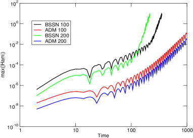
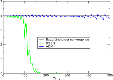
Figure 7: Comparison of the $L_{\infty}$ norm of the Hamiltonian constraint for ADM vs. BSSN. For the purpose of presentation the time coordinate has been adjusted to coincide with the number of crossing times. The left figure shows the growth of the $L_{\infty}$ norm of the Hamiltonian constraint on a double logarithmic scale, the right figure shows the ratios of the $L_{\infty}$ norm of the Hamiltonian constraint for resolutions of 100 and 200 points. A value of $4$ would mark exact second order convergence.

V Discussion

We have presented a program to develop a suite of standardized testbeds for numerical relativity, and a first round of tests. All tests are specified in great detail which extends to numerical methods, grid setup and choice of output quantities to facilitate comparisons. The tests are based on vacuum solutions and periodic boundaries. Even in this simple setup, the design of tests is a highly nontrivial task and several subtle issues require careful consideration: The effects of gravitational collapse introduce considerable subtleties in tests of general relativity with periodic boundary conditions and have been discussed in some detail. Comparing runs for spacetimes which possess symmetries in different setups where the symmetry is manifest, disguised by a coordinate transformation, or disguised by adding random noise can help to understand the problem of what one can learn from simple one-dimensional tests, and help test different aspects of a code. In particular, this has been found useful in separating problems connected to ill-posedness from other sources of instability or inaccuracy.

Several of the tests presented here have been used previously in one form or another, but we have tried to improve their specifications in order to increase their practical value. We have modified the robust stability test based on random noise as presented in Szilagyi et al. (2000) to reduce computational resources when comparing different resolutions and added such a comparison as an integral part of the test. Our setup of the collapsing polarized Gowdy wave test combines a particularly simple choice of initial data with a simple form of the exact solution.

The art of interpreting testbed results requires mastery of the art of interpreting spacetimes. The latter has to be applied both to the continuum limits and to the discretized approximations in order to understand results. A simple example is provided by the gauge wave test, where individual runs may exhibit collapse or expansion as a result of a physical instability of the exact solution. Clearly, a valid code still has to show convergence to this unstable exact solution. We strongly emphasize the importance of comparing results for different resolutions. In particular, convergence tests not only exhibit plain coding errors or numerical instabilities, but it is important to obtain convergence information for all simulations individually, for the whole length of a run. This is illustrated by our comparison of an ADM and a BSSN code for the collapsing Gowdy test. Also, we emphasize that it is not sufficient to monitor constraints to analyze instabilities, but further quantities need to be analyzed to render possible scientifically valuable conclusions.

We have carried out sufficient experimentation with these tests to ensure that they can be implemented with reasonable computational resources and that they can effectively discriminate between the performance of different codes. A separate paper presenting and interpreting test results for codes of all groups that wish to participate will be prepared at a later date. At present, we invite all numerical relativity groups to submit results and join as co-authors in this next paper.

Information on submitting results can be found at the web site www.ApplesWithApples.org. Instructions can also be found there for accessing the results submitted by the various participating groups. We also encourage groups to submit results from tests that go beyond the ones proposed here and that reveal further insight into code performance. This would be particularly helpful in the design of future tests. Also, information concerning forthcoming workshops, and contact information for the participating groups, are posted on the website.

The tests presented here are not intended to be an exhaustive or even minimal list of tests that should be applied to a particular formulation or code. However, they are sufficiently simple and general to allow all groups to compare results with reasonable computational effort. They provide a way of rapidly checking the utility of a code or formulation in situations where detailed theoretical analysis is not possible. The tests also allow isolation of problems of different origin, such as the mathematical formulation, the choice of gauge or the inaccuracy of the numerical method. They do this in a simple situation where cross-comparison with other codes can suggest remedies.

We are proposing here the first step toward establishing a community wide resource which will allow all groups to profit from each other’s successes and failures. Broad participation is essential to the success of this goal. Future workshops, along the lines of the first Mexico workshop, are being planned. The key challenge for the next round of tests will be to include the significantly more complex problem of boundaries.