Tensorial perturbations in an accelerating universe

Abstract

We study tensorial perturbations (gravitational waves) in a universe with particle production (OSC).

The background of gravitational waves produces a perturbation in the redshift observed from distant sources. The modes for the perturbation in the redshift( induced redshift ) are calculated in a universe with particle production.

Key words - gravitational waves, perturbations, induced redshift.

1 Introduction

The inflationary paradigm indicates that we live in a flat universe, but observations from the cosmic microwave background anisotropy detected only $30\%$ of the material content necessary for the density parameter to reach the unity. The non-luminous matter around the galaxies is insufficient to complete the deficit of $70\%$ of the material content of the universe.

The recent measurements on magnitude and redshift of supernovae type Ia, made independently by Perlmutter et al. (1999)[1] and Riess et al. (1998)[2], indicates that our universe is accelerating. Generally, this acceleration is thought to be due to any kind of repulsive gravity , which can be introduced via a negative pressure in the perfect fluid representation of the universe. So, some candidates to this kind of energy are discarded, namely: neutrinos, kinetic energy, radiation. All described by a positive pressure.

To supply the energetic deficit of the universe perhaps we live in a universe dominate by a cosmological constant [3] or a scalar field component, denominate quintessence [4],[5], [6]. The quintessence models are an advantageous alternative to the cosmological constant, due the relation with the super symmetric models [7], the problem of the fine-tuning of the cosmological constant [8] and supergravity models [9].

On another hand, a negative pressure can be provided in the perfect fluid energy momentum tensor, taking into account a cosmological particle production. The cosmological scenario with particle production, denominated by open system cosmology (OSC), was introduced by Prigogine et. al [10] with the intention of solving the problem of entropy content in the universe. Note that, Einstein’s equations can hardly provide an explanation for the origin of the cosmological entropy, since they are purely adiabatic and reversible.

Traditionally the variables describing the cosmological fluid are the energy-density ($\rho$) and the themodynamical pressure ($P_{th}$). In OSC a supplementary variable, the particle number density, enters into the description via a continuity equation with a source of particles. Naturally, the pressure in the stress energy tensor is reinterpreted and a pressure due to the particle creation is added to the thermodynamical pressure, called pressure creation ($P_{c}$).

Considering the source of particles proportional to the product of the number density and Hubble function, the prediction of the actual value for the rate of the particle production is $10^{-16}nucleons/cm^{3}/Yr$ [11]. It is nearly the rate predicted by steady-state model [12]. Otherwise, it is far below the detectable limit, the consequences for the dynamics of the universe can be evaluated. OSC can produce solutions for the very early universe, free of the singularity [13], [10]. Besides that, it can generate inflationary models without the difficulties associated with supercooling [14] and lead to a universe sufficiently old as to agree with observations [15] [16].

So, we consider the OSC framework an promising background, from the observational point of view, to study cosmological perturbations.

The interest in the study of cosmological tensorial perturbations has increased due to the realization that they contribute to the anisotropy of the cosmic microwave background radiation [17], [18], [19], [20],[21].

Gravitational waves provide a new perspective of the observable universe. The energy density of gravitational waves can affect matter, however weakly, causing density fluctuations, peculiar velocities and tidal distortions, for example. On the another hand, a cosmological background of gravitational waves induces redshift perturbations and angular deviations in light transversing it. The observations, at present, do not distinguish among anisotropies due density perturbations and those produced by gravitational waves at recombination era.

In this work we solve the differential equation for tensorial modes in a synchronous gauge for a cosmological background with particle production.

The redshift fluctuations ($\tilde{Z}$) induced by the gravitational waves in OSC background for an accelerated and non-accelerated universe are calculated.

2 Background

2.1 Open system cosmology

In this section I attempt to give a summary of OSC basic equations. The universe will be considered homogeneous and isotropic, described by the FRW line element

$$ds^{2}=R^{2}(\eta)\{d\eta^{2}-(dr^{2}+r^{2}d\theta^{2}+r^{2}\sin{\theta}^{2}d\phi^{2})\}\,.$$ (1)

The Einstein field equations for the space-time described by the line element above and the usual energy momentum tensor of an ideal fluid with an additional pressure [10] due to the particle production ($P_{c}$) are given by

$$3(\frac{{R}^{\prime}}{R})^{2}=\kappa R^{2}\rho$$ (2)

$$-2\frac{{R^{\prime\prime}}}{R}-\frac{{R}^{\prime}}{R}=\kappa R^{2}P=\kappa R^{2}(P_{th}+P_{c})\,,$$ (3)

where the prime means derivative with respect to the conform time $\eta$, and $\kappa=8\pi G$, $\rho$ is the energy density, $P_{th}$ is the thermodynamical pressure, and $P_{c}$ is the creation pressure.

The field equations (2) and (3) are coupled with the balance equation for the particle number density

$${n}^{\prime}+n\theta=\Psi\,,$$ (4)

where $\theta=3\frac{{R^{\prime}}}{R}$ and $\Psi$ is the source of the particle production.

The process of transference of the energy from the gravitational field to the production of particles acts as a source of entropy. Using Gibbs relation, the energy conservation law ($u^{\alpha}{T^{\alpha\beta}}_{;\beta}=0$, where $u^{\alpha}$ is the velocity four-vector) and balance equation for the particle number density, it is readily obtained that

$${S^{\alpha}}_{;\alpha}=n\dot{\sigma}+\sigma\Psi=\frac{-P_{c}\theta}{T}-\frac{\mu\Psi}{T}\,,$$

where $\sigma$ is the entropy per particle, $S^{\alpha}$ is the entropy current, $\mu=\frac{\rho+P_{th}}{n}-T\sigma$ is the chemical potential, $T$ is the temperature, and the dot means the usual time derivative. Considering the process as adiabatic ( $\dot{\sigma}=0$ ) the pressure creation is given by [22]

$$P_{c}=-\frac{\rho+P_{th}}{n\theta}\Psi\,.$$ (5)

Combining equations (2), (3), (4) and the state equation

$$P_{th}=\nu\rho\,,$$

where $\nu$ is a constant, it follows that

$$R{R^{\prime\prime}}+[(\frac{3\nu+1}{2})-\frac{(\nu+1)\Psi}{2nH}]{R}^{\prime 2}=0\,.$$ (6)

In order to integrate equation (6) we write out an expression for the source $\Psi$. Following Lima et al. [14], a physically reasonable expression for the particle creation rate is $\Psi=3n\beta H$. To have the characteristic time for matter creation the Hubble time itself, $\beta$ must be constant. Beyond this, $\beta$ must be a positive constant, otherwise the second law of thermodynamics (${S^{\alpha}}_{;\alpha}>0$) is violated. So, integrating (6) the expansion of the universe is governed by the scale factor

$$R=\{R_{0}(\frac{\eta}{\eta_{0}})\}^{\frac{2}{3(1-\beta)(\nu+1)-2}}\,,$$ (7)

where

$$R_{0}={{{\frac{3(1-\beta)(\nu+1)-2}{2}}(\frac{N_{0}^{\nu+1}m}{3})^{\frac{1}{2}}\eta_{0}}}^{\frac{2}{3(1-\beta)(\nu+1)-2}}\,.$$ (8)

The subscript $0$ is relative to the present time, $m$ is the mass of produced particle and $N$ is the particle number.

The universe that evolves according the scale factor (7) emerges from a singularity. However, in the work of the Prigogine et al. [10], the source of the particles is proportional to the square of the Hubble function and the universe emerges from an initial instability given by an initial number of particles, instead of a singularity.

2.2 Acceleration of the universe

According to data from type Ia supernovae observations, the universe is accelerating[23]. Generally, a negative pressure is responsible for the increase of the expansion velocity of the universe and can be generated from the inclusion of the cosmological term [3] or using a quintessence component [24], for example.

An alternative view would be to consider particle creation, which naturally redefine the energy-momentum tensor and could account for this increasing expansion velocity. Taking into account (6), we can write the deacceleration parameter[25] in terms of the particle source function, namely

$$q=\frac{1}{2}-\frac{4\pi mG\Psi}{H^{3}}\,,$$ (9)

where $m$ is the rest mass of the produced particles, and we consider a null value for the curvature. Considering $\Psi=3n\beta H$, we obtain an accelerated universe, expanding with the scale factor (7), if $\beta>\frac{1}{3}$ [11].

3 Tensorial modes

The background is described by the line element (7). In order to obtain the perturbed field equations for tensorial modes, we must to return to the original field equations, substituting $\tilde{g}_{\mu\nu}=g_{\mu\nu}+h_{\mu\nu}$, where $g_{\mu\nu}$ is the background solution and $h_{\mu\nu}$ is a perturbation around $g_{\mu\nu}$. The perturbed field equations are [25]

$$\delta R_{\mu\nu}=-8\pi G\delta S_{\mu\nu}\,,$$ (10)

where $S_{\mu\nu}=T_{\mu\nu}-\frac{1}{2}g_{\mu\nu}{T^{\lambda}}_{\lambda}$, and $T_{\mu\nu}$ is the energy momentum tensor. Therefore, the equation for evolution of the tensorial modes in a synchronous gauge is given by [26]

$$h^{\prime\prime}-2\frac{R^{\prime}}{R}h^{\prime}+[n^{2}-2(\frac{R^{\prime\prime}}{R}-\frac{R^{\prime 2}}{R^{2}})]h=0\,,$$ (11)

where the spatial dependence of the perturbed quantities are given in terms of spherical harmonics

$$\nabla^{2}h_{ij}(x,\eta)=-h(\eta)n^{2}Q_{ij}\,.$$

$Q_{ij}$ is tracelles transverse eigenfunction in 3-d spatial section, so that $\nabla^{2}Q_{ij}=-n^{2}Q_{ij}$.

Substituting the scale factor (7) in equation (11), we find

$$h_{a}=C_{1}\eta^{k_{1}}J_{w}(n\eta)\,,$$ (12)

$$h_{b}=C_{2}\eta^{k_{1}}Y_{w}(n\eta)\,,$$ (13)

where $C_{1}$ and $C_{2}$ are integrations constants,

$$k_{1}=\frac{1}{2}\frac{3(\beta-1)(\nu+1)-2}{3(\beta-1)(\nu+1)+2}$$ (14)

and

$$w=\frac{3}{2}\frac{\beta(\nu+1)-\nu+1}{3\beta(\nu+1)-3\nu-1}\,.$$ (15)

The functions $J$ and $Y$ are the Bessel functions of the first and second kind respectively.

The evolution of the tensorial modes (12) and (13) will depend of the parameter $\beta$. Consequently, will depend on the deacceleration parameter (9).

For an accelerated matter dominated universe ($\beta>\frac{1}{3},\nu=0$), we have oscillatory decaying modes (Fig. 1 ).

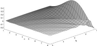
Figure 1: Evolution of the mode (12) for $\beta=\frac{5}{9}$ and $\nu=0$.

On the other hand, for a non-accelerated universe we have oscillatory growing modes (Fig. 2 ).

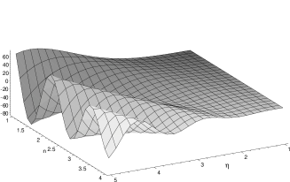
Figure 2: Evolution of the mode (13) for $\beta=\frac{1}{9}$ and $\nu=0$.

For the radiation dominated era the profiles of the tensorial modes are similar to the matter dominated era.

The integration, for the large scale perturbations ($n\rightarrow 0$), of the equation (11), furnishes the growing mode:

$$h_{1}(\eta)=C_{1}\eta$$ (16)

and a mode dependent of the creation parameter

$$h_{2}(\eta)=C_{2}\eta^{\frac{-4}{3\beta(\nu+1)-3\nu-1}}\,.$$ (17)

From observational point of view the large scale perturbation has some advantages. The measure of the anisotropy of cosmic microwave background radiation is well established for $n\rightarrow 0$, that is, for small value of $l$ , where $l$ denotes the multipolar order in the expansion of the two point correlation function of temperature

$$C(\theta)=\Sigma^{\infty}_{l=2}C_{l}P_{l}(\cos(\theta))\,.$$

Using $0<\beta<\frac{1}{3}$ the universe is non-accelerated and the mode (17) will behave as a growing mode.

4 Induced redshift

How the propagation of light is affected by the less than perfectly symmetric and smooth universe (here gravitational waves) is our goal in this section. Basically, gravitational waves effects can be put in two categories. Direct ones involve energy density of the gravitational waves affecting matter (for example, density fluctuations, peculiar velocities, tidal distortions) and induced effects that act on the propagation of radiation. We calculate the induction, by a cosmological background of gravitational waves, of redshift perturbations in light transversing it in a universe with particle production. The induced effect on the reshift is given by the relation [27] [28]

$$Z=\frac{R_{0}}{R}-1+\tilde{Z}\,,$$ (18)

where

$$\tilde{Z}=-\frac{R_{0}}{2R}{\int}^{\eta}_{0}\frac{\partial h_{11}}{\partial\eta}d\eta\,.$$ (19)

Writing $h_{ij}=F(t)\exp{i\vec{k}\centerdot\vec{x}}$, where $\vec{x}$ is the comoving distance and $\vec{k}$ is the comoving wave vector, given by $k=\frac{2\pi R}{\lambda}$, and considering the large wavelength perturbations, we obtain the induced redshift for the tensorial perturbations (16) and (17), respectively:

$$\tilde{Z}_{1}=C_{1}\eta^{\frac{3(1-\beta)(1+\nu)-4}{3(1-\beta)(\nu+1)-2}}$$ (20)

and

$$\tilde{Z}_{2}=C_{2}\eta^{\frac{2}{3(1-\beta)(\nu+1)-2}}\,.$$ (21)

The induced redshift is a first order effect in the amplitude perturbations, altering our perception of the universe, not the physical constituents themselves. Note that these perturbations in the redshift are dependents of the creation parameter $\beta$, consequently these modes are affected by the acceleration of the universe.

Similarities of this effect with gravitational lensing was point out by E. Linder [28]

5 Conclusions

The particle production in the universe results in a reinterpretation of the energy momentum tensor. The ordinary pressure is modified and divided in thermodynamic pressure and a negative pressure due to the creation of particles.

The cosmological particle creation furnishes an alternative model to explain the increasing of the expansion velocity of the universe and furnishes an suitable estimative for the age of the universe. Taking into account the scale factor (7) the Hubble function is given by

$$H=\frac{2}{3(1-\beta)(1+\nu)t}\,.$$

If we do not violate the dominant energy condition and the second law of thermodynamics the constant $\beta$ stay in the interval $0\leqslant\beta<1$. Note that, for this interval of $\beta$, the universe will be older than the universe described by standard model without creation ($\beta=0$). Consequently, the conflict between the age of the universe and the age of the oldest stars in our galaxy is eliminate in OSC [16], [29]. So, we consider OSC an promising background from the observational point of view to realize perturbations.

We obtain the tensorial modes, for large wavelength perturbations and modes dependent on the scale of the perturbations, considering the OSC as a background. The behavior of these modes are sensitive to the creation parameter and consequently to the dynamics of the universe. Taking into account $\beta=0$ we obtain the usual solution for the ordinary fluid without particle production.

The induced redshift ( $\tilde{Z}$) due to the cosmological gravitational waves are determined for large wavelength perturbations. The induced effects are small, but potentially observable. The induced redshift can be , in principle, used to clarify the dynamics of the expansion of the universe, include for redshift $z>>1$.

Analyzing the induced redshift expressions,eq. (20) and eq. (21), we conclude that, if we live in a deaccelerated universe ($\beta<\frac{1}{3}$) eq. (20) is a decaying mode and eq. (21) a growing mode. Otherwise, for an accelerated universe ($\beta>\frac{1}{3}$) we obtain the inverse behaviour for the induced redshift. So, the induced redshift for more distant objects is greater than the close objects, this seems plausible.

The growing mode for the induced redshift (eq.(21)) can contributes for give us an impression that the observed object has a redshifit greater than the expected in a universe without the background of tensorial perturbations, even than we lived in a deaccelerated universe ($\beta<\frac{1}{3}$).

The contribution of gravitational waves, generated in a universe with particle creation, in the anisotropy of the cosmic microwave background radiation is subject for a future study.

6 Acknowledgments

I like to acknowledgment to the Brazilian agency (CNPQ) for the financial support.

References

- [1] S. Perlmutter et al., Astrophys. J, 517 , 565 (1999).
- [2] A. G. Riess et al., Astron. J., 116 , 1009 (1998).
- [3] Sean M. Carrol astro-ph/ 0004075 (2000).
- [4] R. R. Caldwell, R. Dave and P. J. Steinhardt, Phy. Rev. Lett., 80 , 1582, (1998).
- [5] R. R. Caldwell and P. J. Steinhardt, Phys. Rev. D, 57 , 6057, (1998).
- [6] L. Wang and P. J. Steinhardt, Astrophys. J., 503 , 483, (1998).
- [7] P. Bin truy, Phys. Rev. D, 60 , 063502, (1999).
- [8] C. Kolda and D. Lyth, Phy. Lett. B, 458 , 197, (1999).
- [9] P. Brax and J. Martin, Phy. Lett. B, 468 , 40, (1999).
- [10] I. Prigogine, J. Geheniau, E. Gunzig and P. Nardone, Gen. Relat. Grav., 21 , 8, (1989).
- [11] J. A. S. Lima and J. S. Alcaniz, Astron. Astrophys., 348 , 1, (1999).
- [12] F. Hoyle, G. Burbidge, J. V. Narlikar, Astrophys. J., 410 , 437, (1993).
- [13] L. R. W. Abramo and J. A. S. Lima, Class. Quantum Grav., 13 , 2953, (1996).
- [14] J A. S. Lima, A. S. Germano and L. R. W. Abramo, Phys. Rev. D , 53, 4287, (1996).
- [15] J. A. S.Lima and J. S. Alcaniz, Astron. Astrophys. 348 , 1, (1999).
- [16] M. de Campos and N. Tomimura, Brazilian Journal of Physics, 468 , 3, (2001).
- [17] F. Atrio-Barandela and J. Silk, Phys. Rev. D, 49 , 1126, (1994).
- [18] M. S. Turner and M. White, Phys. Rev. D , 53 , 6822, (1996).
- [19] M. S. Turner, Phys. Rev. D, 55 , 435, (1997).
- [20] L. P. Grishchuk, Phys. Rev. D, 53 , 6784, (1996).
- [21] L. P. Grishchuk, Phys. Rev. D, 50 , 7154, (1994).
- [22] M. O. Calv o, J. A. S. Lima and I. Waga, Phy. Lett. A, 162 , 223, (1992).
- [23] A. Goobar , Nuc. Phys. B 95, 8, (2001).
- [24] M. Signore and D. Puy , New Astronomy Reviews 45, 409, (2001).
- [25] S. Weinberg, Gravitation and Cosmology, (Jonh Wiley & Sons, New York,1972).
- [26] J. C. Fabris and S. V. de B. Gonçalves, Class. Quantum Grav. 16 , 2269, (1999).
- [27] Eric Linder, Astrophys. J. 326, 517, (1988).
- [28] Eric Linder, Astrophys. J., 328, 77, (1988).
- [29] B. Chaboyer, Astrophys. J., 494, 96, (1998).