Global structure of Choptuik’s critical solution in scalar field collapse

Abstract

At the threshold of black hole formation in the gravitational collapse of a scalar field a naked singularity is formed through a universal critical solution that is discretely self-similar. We study the global spacetime structure of this solution. It is spherically symmetric, discretely self-similar, regular at the center to the past of the singularity, and regular at the past lightcone of the singularity. At the future lightcone of the singularity, which is also a Cauchy horizon, the curvature is finite and continuous but not differentiable. To the future of the Cauchy horizon the solution is not unique, but depends on a free function (the null data coming out of the naked singularity). There is a unique continuation with a regular center (which is self-similar). All other self-similar continuations have a central timelike singularity with negative mass.

I Introduction

In general relativity, a black hole may be formed during the evolution from asymptotically flat initial data where none is present. Consider a one-parameter family of regular asymptotically flat initial data. It is not difficult to find such families which form a black hole for some range of the parameter (strong data) but disperse for another range (weak data). The boundary between the two regimes is the black hole threshold. In what is called type II critical collapse, the black hole mass can be made arbitrarily small by adjusting the parameter $p$ of the initial data to its critical value $p_{*}$. Near the threshold, the final black hole mass $M$ then scales as

$$M\simeq C(p-p_{*})^{\gamma}$$ (1)

where $C$ is a constant. $C$ depends on the family, but the transcendental number $\gamma$ is universal – it depends on the type of matter but not on the family of initial data.

Type II critical collapse was originally discovered by Choptuik in the spherically symmetric massless scalar field Choptuik , but has since been found in many simple matter systems in spherical symmetry, and also in axisymmetric gravitational waves AbrahamsEvans . A review of the field is critreview .

Type II critical phenomena can be described in dynamical systems terms: the phase space of the system has (at least) two attracting fixed points, namely black holes and dispersion. The boundary between the two basins of attraction, the critical surface, contains a critical point: it is an attractor within the boundary surface, and a repeller only in the one remaining direction. This means that it must have precisely one unstable linear perturbation, with the property that adding a bit of that perturbation with one sign leads to collapse, while adding it with the opposite sign leads to dispersion. In type II critical collapse the critical point is either a discretely self-similar (DSS) or a continuously self-similar (CSS) spacetime.

Type II critical collapse is interesting, among other things, because the maximum value of the curvature in a subcritical evolution, and the maximal value of the curvature outside the black hole in a supercritical evolution, both diverge as

$$(R_{abcd}R^{abcd})_{\rm max}\sim|p-p_{*}|^{-4\gamma}$$ (2)

as the fine-tuning is improved. (This is basically the same result as the black hole mass scaling, and similar results hold for any curvature invariant.) From the dynamical systems picture it is clear that the end point of type II critical collapse in the limit of perfect tuning of $p$ to its critical value $p_{*}$ is not a “zero mass black hole” but the critical solution itself. This solution has a naked singularity. It is therefore interesting to examine the global spacetime structure of the critical solution, and in particular its Cauchy horizon. Here we do this for the spherically symmetric massless scalar field, where the critical solution is DSS. We focus on this system because CSS can be viewed as a limiting case of DSS, and because the critical solution in the most interesting system in which type II critical phenomena have been found, axisymmetric pure gravity, is also DSS AbrahamsEvans .

In Section II we discuss the global structure of Choptuik’s critical solution kinematically. Section III sets out the field equations for the real massless scalar field in spherical symmetry, in coordinates adapted to our problem, and describes the mathematical structure of the solution at the Cauchy horizon of the singularity. Sections IV, V and VI show the results of our numerical integration of the critical solution, and Section VII contains our conclusions. Some technical details have been removed to appendices.

II Kinematical discussion

A spacetime is discretely self-similar (DSS) if there is a conformal isometry $\Phi$ of the spacetime such that

$$\Phi_{*}g_{ab}=e^{-2\Delta}g_{ab}.$$ (3)

The value of the dimensionless “logarithmic scale period” $\Delta$ is a geometric property of the spacetime, independent of coordinates. It is often useful to work in coordinates adapted to the symmetry at hand. A generic self-similar and spherically symmetric metric can be written as

$$ds^{2}=e^{-2\tau}\left(A\,d\tau^{2}+2B\,d\tau\,dx+C\,dx^{2}+F^{2}\,d\Omega^{2}\right)$$ (4)

where $d\Omega^{2}=d\theta^{2}+\sin^{2}\theta\,d\varphi^{2}$ is the metric on the unit 2-sphere, and where $A$, $B$, $C$ and $F$ are functions of $\tau$ and $x$. This metric is DSS if and only if they are periodic in $\tau$ with period $\Delta$. It is continuously self-similar (CSS) if these functions are completely independent of $\tau$. We assume that the signature is $(-,+,+,+)$, and that the metric is non-degenerate. This leads to the inequality $AC-B^{2}<0$. We also assume $F\geq 0$ for definiteness.

Any four-dimensional spacetime splits into a product of a two-dimensional spacetime (the reduced manifold) and a round two-sphere of area $4\pi r^{2}$. The area radius $r$ is a scalar in the reduced manifold. Here the coordinates on the reduced manifold are $\tau$ and $x$, and the area radius is given by $r=e^{-\tau}F$. Geodesics in the reduced spacetime are radial (constant $\theta$ and $\varphi$ geodesics in the full spacetime). The Hawking mass $m$ is defined by $1-2m/r=(\nabla r)^{2}$. It is a scalar on both the full and the reduced spacetime. From $m$ we define the two dimensionless scalars $\mu=2m/r$ and $a=(1-\mu)^{-1/2}$. It is easy to show that a spherical surface where $\mu\geq 1$ is a closed trapped surface, and one where $\mu=1$ is an apparent horizon. In a DSS spherical spacetime, $\mu$ and $a$ are periodic in $\tau$.

Radial null geodesics which are invariant under the symmetry (3) are called self-similarity horizons (SSH). They are the key to determining the causal structure. All coordinate systems of the form (4) are related by coordinate transformations of the form

$$x^{\prime}=\varphi(\tau,x),\qquad\tau^{\prime}=\tau+\psi(\tau,x),$$ (5)

where $\varphi$ and $\psi$ are periodic in $\tau$ with period $\Delta$. We use this coordinate freedom to make all lines in the reduced manifold where $F=0$ into lines of constant $x$. (These can be either regular centers or central singularities.) We also make all SSHs into lines of constant $x$ where $A=0$.

In order to discuss the global structure of the Choptuik spacetime and its possible continuations we briefly review the kinematical results of spherical_dss . In a spherically symmetric DSS spacetime, two kinds of singularities can be distinguished. From dimensional analysis it can be seen that the Kretschmann scalar scales as $e^{4\tau}$ for constant $x$, and therefore the set $\tau=\infty$ is a central (because $r$ scales as $e^{-\tau}$) curvature singularity. We call this the kinematical singularity. Geometrically, this singularity is either a point or a null line in the reduced spacetime. There are two types of self-similarity horizons that in spherical_dss we have called fans and splashes. The kinematical singularity is null if there is at least one splash. Additional central singularities can arise where $F=0$ for all $\tau$. (We call these dynamical.) Because $\tau$ takes all values up to $\infty$ they are connected to the kinematical singularity. There are at most two of them, connected to the kinematical singularity at its ends. Topologically, they are lines in the reduced manifold.

All known type II critical solutions in spherical gravitational collapse can be defined by the properties of self-similarity (CSS or DSS), analyticity at the past lightcone, and the requirement that they have a single unstable perturbation mode. A generic spherically symmetric DSS scalar field solution is singular either at the center or the past lightcone. Imposing analyticity at both the center and the past lightcone defines a nonlinear PDE boundary value-problem which admits at most discrete solutions critscalar . Only one such solution has been found, and it empirically turns out to have only one unstable mode, and to agree perfectly with the critical solution found previously in collapse simulations by Choptuik Choptuik .

The global structure of the Choptuik solution up to the future light cone of the kinematical singularity (which is a Cauchy horizon) is sketched in Fig. 1, together with the $x$ and $\tau$-lines of the three coordinate patches that we shall use in the numerical calculations. This structure is the same as for all other known type II critical solutions in spherical symmetry. These solutions have a regular center $x=x_{c}$ in the past. As $x$ increases, the $x$ lines are at first timelike, so that $A<0$. They become null at the fan $x=x_{p}$ where $A=0$, $\partial A/\partial x>0$ and $B>0$. As $x$ increases further, they are spacelike, so that $A>0$ spacelike. Somewhere in the spacelike region $B$ changes sign. The $x$-lines become null again at the second fan $x=x_{f}$, where $A=0$, $\partial A/\partial x<0$ and $B<0$. Approaching the kinematical singularity $\tau=\infty$ from the range of “angles” $x_{c}\leq x\leq x_{f}$ it is a single point. $x_{p}$ and $x_{f}$ are its past and future lightcones.

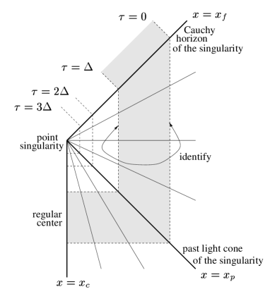
Figure 1: (Uncompactified) conformal diagram of the critical solution up to the Cauchy horizon showing DSS-adapted coordinates. DSS lines are shown continuous. Lines of constant $\tau$ are shown dashed (we have assumed $e^{\Delta}=2$ while in reality $e^{\Delta}\simeq 31$). Note that the numerical domain is $0\leq\tau<\Delta$ (shaded), with periodic boundary conditions. We have illustrated the three coordinate patches we use for numerical work: in the past patch between $x_{c}$ and $x_{p}$ $\tau$-lines are spacelike. In the outer patch between $x_{p}$ and $x_{f}$ $\tau$-lines are timelike. In the future patch beyond $x_{f}$ they are null. The three patches together cover the entire spacetime without overlapping, and the coordinates $x$ and $\tau$ are continuous at the interfaces.

We demonstrate below numerically that the curvature at the Cauchy horizon $x=x_{f}$ is finite in Choptuik’s scalar field critical solution. Furthermore all geodesics cross it in finite affine parameter. The spacetime can therefore be extended beyond, but this continuation is not unique. Mathematically speaking we shall see that the solution is not analytic at the Cauchy horizon in the limit coming from the past, and so there is no preferred analytic continuation to the future. (The curvature is only $C^{0}$ from the past.) The family of continuations in which the curvature is $C^{0}$ across the Cauchy horizon and which are DSS is parameterized by one free periodic function $\hat{U}_{\epsilon}(\tau)$. Physically speaking this function can be interpreted as data on the naked singularity which determine the continuation, in addition to the null data on the Cauchy horizon.

We now discuss the possible continuations that are allowed kinematically.

Figure 2: An extension with a timelike central singularity. Instead of the central singularity the solution could also have a regular center. This diagram has two fans at $x_{p}$ and $x_{f}$.

In the simplest case, the $x$-lines to the future of the Cauchy horizon are all timelike ($A<0$) until a timelike singularity $F=0$ is reached. In our classification this is a dynamical singularity, while the kinematical singularity is a single point. This conformal structure is shown in Fig. 2. If $m\sim r^{3}$, or equivalently $\mu\sim F^{2}$ as $x\to x_{r}$, the conformal structure is the same, but with the singularity replaced by a regular center.

Nolan Nolan has drawn spacetime diagrams for spherically symmetric CSS spacetimes in which the point singularity at the origin of the Cauchy horizon is only the starting point of an ingoing central null singularity. In our classification this is an extended kinematical singularity, which requires the existence of at least one splash, that is a line where $A=0$ again. Fig. 3 shows the simplest generic possibility, in which the splash is followed by a spacelike dynamical singularity, which covers part of the naked null singularity. This spacetime structure can actually be realized in spherical CSS scalar field solutions OriPiran . The same, and more exotic structures, can also be realized in spherical CSS perfect fluid solutions fluidcss .

Contrary to our expectations, we have found that none of these exotic possibilities are realized as spherical DSS continuations of the Choptuik solution. There is a unique DSS continuation with a regular center, and all other DSS continuations have a timelike singularity. In hindsight, the reason appears to be that the null data on the Cauchy horizon are extremely weak. With stronger data (not associated with the Choptuik spacetime) we find different kinds of continuations.

Figure 3: A hypothetical extension with a null singularity. This diagram has two fans at $x_{p}$ and $x_{f}$ and a splash at $x_{h}$. Note that this extension is not realized as a DSS continuation of the Choptuik solution.

III Coordinates and field equations

In spherical symmetry, there are four algebraically independent Einstein equations, which can be taken to be $G_{\tau\tau}$, $G_{\tau x}$, $G_{xx}$ and $G_{\theta\theta}$. The fourth of these is a combination of derivatives of the first three and can therefore be disregarded. The first three equations contain first and second derivatives of $F$, but only first derivatives of $A$, $B$, and $C$. In the following we assume that $F$ is a given function of $x$ and $\tau$. The Einstein equations then determine three independent linear combinations of the six first derivatives of $A$, $B$ and $C$. A non-degenerate basis of this three-dimensional space is $\mu_{,x}$, $\mu_{,\tau}$ and $\nabla_{\mu}\nabla^{\mu}r$. (With $F(\tau,x)$ given, this last term contains only first derivatives of $A$, $B$ and $C$.)

Here we investigate massless real scalar field matter. The scalar field $\phi$ obeys the wave equation

$$\nabla_{a}\nabla^{a}\phi=0,$$ (6)

and the Einstein equations can be written as

$$R_{ab}=8\pi G\,\nabla_{a}\phi\nabla_{b}\phi.$$ (7)

The wave equation, when written as a second order PDE, will in general contain both first derivatives of all four metric coefficients. However, by writing the wave equation in a geometrically defined first-order form, all metric derivatives except one can be eliminated. Define two null derivative operators $\nabla_{u}$ and $\nabla_{v}$ with the usual convention that both point towards the future and that $\nabla_{u}$ points inwards while $\nabla_{v}$ points outwards. Normalize them by imposing that $\nabla_{u}r=-r$ and $\nabla_{v}r=r$. We define the null derivatives of the scalar field as $U=\sqrt{2\pi G}\,\nabla_{u}\phi$ and $V=\sqrt{2\pi G}\,\nabla_{v}\phi$. The massless wave equation in spherical symmetry can then be written as

$$\nabla_{v}U-V+PU = 0,$$ (8)

$$\nabla_{u}V+U-PV = 0,$$ (9)

with the scalar $P\equiv r\nabla^{2}r/(\nabla r)^{2}=a^{2}-1$. Using the Einstein equations, the curvature can be given in terms of $U$ and $V$:

$$R_{uu}=4U^{2},\quad R_{vv}=4V^{2},\quad R_{uv}=4UV,$$ (10)

(other components of the Ricci tensor vanish) and

$$R=\frac{-4}{a^{2}r^{2}}UV.$$ (11)

The most general form of the scalar field compatible with DSS is

$$\phi(\tau,x)=\psi(\tau,x)+\kappa\tau$$ (12)

where $\psi(\tau+\Delta,x)=\psi(\tau,x)$ and $\kappa$ is a global constant. In the Choptuik solution, $\kappa=0$ empirically, so that $\phi$ is periodic in $\tau$. This means that $U$ and $V$ have zero average in $\tau$. Moreover, $U$ and $V$ in the Choptuik solution obey $U(\tau+\Delta/2,x)=-U(\tau,x)$ and so for $V$. (This of course implies zero average.) As a consequence $\mu(\tau+\Delta/2,x)=\mu(\tau,x)$ and so for other suitable metric fields. We shall assume these extra symmetries in our numerical work, but all our analytical expressions remain valid if these symmetries are dropped.

We now describe three coordinate patches that cover the critical solution. We demand that both the past and the future lightcones of the singularity occur at lines of constant $x$. This makes it easier to impose regularity at the center and past lightcone, and to investigate the behavior at the future lightcone (Cauchy horizon). It also allows us to match the coordinate patches without overlap. Subject to these requirements, we have tried to make the field equations in each patch as simple as possible. Based on the three patches, it is straightforward to construct a single smooth coordinate system covering the whole spacetime (see Section VI), but using it from the beginning would unnecessarily complicate our numerical work. We summarize a number of coordinate systems for spherically symmetric CSS and DSS spacetimes, and their advantages and disadvantages, in the Appendix.

III.1 Past patch

On the past patch, which extends from the regular center to the past lightcone, we write the metric in terms of two free functions $f(\tau,x)$ and $a(\tau,x)$ as

$$A=a^{2}(x^{2}-f^{2}),\qquad B=-xa^{2},\qquad C=a^{2},\qquad F=x,$$ (13)

for $x\geq x_{c}\equiv 0$. Here $a=(1-2m/r)^{-1/2}$ is the scalar we defined above. These coordinates can be derived from the Schwarzschild-type metric

$$ds^{2}=-\alpha^{2}\,dt^{2}+a^{2}\,dr^{2}+r^{2}\,d\Omega^{2}$$ (14)

through the coordinate change $x=r/(-t)$ and $\tau=-\ln(-t)$, and defining $f=\alpha/a$. The remaining gauge freedom of time relabelling is fixed by imposing that the past lightcone is on a constant $x=x_{p}$ line. Note that we do not follow the convention of Choptuik that $\alpha=1$ at the center, which in critscalar forced us to introduce an additional free function of time in the definition of $x$. The Einstein equations are

$$f_{,x} = {(a^{2}-1)f\over x},$$ (15)

$$(a^{-2})_{,x} = {1-(1+U^{2}+V^{2})a^{-2}\over x},$$ (16)

$$(a^{-2})_{,\tau} = \left[{(f+x)U^{2}-(f-x)V^{2}\over x}+1\right]a^{-2}-1,$$ (17)

and the matter equations are

$$U_{,x} = {f[(1-a^{2})U+V]-{xU_{,\tau}}\over x(f+x)},$$ (18)

$$V_{,x} = {f[(1-a^{2})V+U]+{xV_{,\tau}}\over x(f-x)},$$ (19)

At the regular center $x=0$ we impose elementary flatness, that is the absence of a conical singularity. In order to do this, we define $\Pi=(V+U)/(2x)$ and $\Psi=(V-U)/(2x^{2})$ and impose that both are regular even functions of $x$ at $x=0$. At the past lightcone we have $f-x=0$, which by our gauge choice means that $f=x_{p}$ there. We also impose the physical regularity condition

$$V_{,\tau}-(1-a^{2})V-U=0$$ (20)

on the past lightcone. The conditions of DSS, regularity at the center and regularity at the past lightcone select a solution. The equations on the past patch are form-invariant under the linear coordinate transformation $x\to cx$, $f\to cf$, and $a$, $U$ and $V$ unchanged. In the numerical results presented here we have set $x_{p}=1$ on the past patch. Note that the regularity condition (20) is coordinate-independent, as $U$, $V$ and $a$ and $r$ are all scalars and $\tau=-\ln r$ on the lightcone.

III.2 Outer patch

On the outer patch, which extends from the past to the future lightcone, we write the metric in terms of $a(\tau,x)$, $b(\tau,x)$, and the auxiliary function $\xi(\tau)$ as

$$A=a^{2}(1-b^{2}),\qquad B=a\,b\,\xi,\qquad C=-\xi^{2},\qquad F=1,$$ (21)

where $\xi>0$ is a function of $\tau$ only. $a>0$ is the scalar defined above. We fix the remaining gauge freedom by imposing that the past lightcone $b=-1$ occurs at $x=x_{p}$, and the future lightcone $b=1$ at $x=x_{f}$. Putting both lightcones on a line of constant $x$ requires $\xi(\tau)$ to be non-constant. There is no outer coordinate patch that does not have at least one function like $\xi(\tau)$. As $\tau=-\ln r$ everywhere on the outer patch, $\tau$ is continuous between the past and outer patches.

The metric equations are

$$\frac{b_{,x}}{\xi} = -\frac{-3+a^{2}+U^{2}(1-b)+V^{2}(1+b)}{2a}-\frac{\xi^{\prime}}{a\xi}\;,$$ (22)

$$\frac{a_{,x}}{\xi} = -\frac{U^{2}-V^{2}}{2},$$ (23)

$$\left(a^{-2}\right)_{,\tau} = \left[1+U^{2}(1-b)+V^{2}(1+b)\right]\,a^{-2}-1,$$ (24)

and the matter equations are

$$\frac{U_{,x}}{\xi}=\frac{(1-a^{2})U+V+U_{,\tau}}{a(1-b)},$$ (25)

$$\frac{V_{,x}}{\xi}=-\frac{(1-a^{2})V+U+V_{,\tau}}{a(1+b)}.$$ (26)

Note that the $a_{,\tau}$ constraint equation is again linear in $a^{-2}$. The equations on the outer patch are form-invariant under the linear coordinate transformation $x\to cx+d$, $\xi\to\xi/c$, and $a$, $b$, $U$ and $V$ unchanged. In the numerical results presented here we have set $x_{p}=-1$ and $x_{f}=1$ on the outer patch.

III.3 Singular behavior at the Cauchy horizon

We shall see that at the Cauchy horizon the solution is mildly singular. Naive finite differencing breaks down there. Instead we expand the generic solution around the Cauchy horizon in terms of two free periodic functions $V_{0}$ and $\hat{U}_{\epsilon}$, and match this expansion to the numerical evolution at a small finite distance to the past of the Cauchy horizon. Before describing the full expansion, we focus on the origin of the singular behavior.

Equation (25) becomes singular at the future lightcone because the denominator of the right hand side vanishes there. In contrast to the past lightcone, we do not have any freedom left to enforce the vanishing of the numerator as well. Therefore we expect the solution to have some kind of singularity at $x_{f}$. We rewrite (25)

$$DU_{,x}-U_{,\tau}-(1-a^{2})U=V,$$ (27)

where we have defined the metric function

$$D\equiv\frac{a(1-b)}{\xi}.$$ (28)

$D$ is positive on the outer patch and vanishes on the future light cone. The characteristics $x(\tau)$ of Eq. (27) are given by

$$\frac{dx(\tau)}{d\tau}=-D\left(\tau,x(\tau)\right).$$ (29)

Recall that we impose the gauge condition that the CH is at $x=x_{f}$, or $b(\tau,x_{f})=1$. We define the shorthand $y=x-x_{f}$.

We now make one fundamental assumption, namely that the spacetime admits regular null data on the Cauchy horizon $y=0$. This assumption is clearly necessary if we want to continue the spacetime through the CH, but here we make it simply because we have not been able to find a more general ansatz. We shall see later that it is sufficiently general to be matched to the critical solution that we have obtained numerically on the past patch.

We therefore assume that $V$ is continuous, or

$$V(\tau,x)=V_{0}(\tau)+o(y^{0}).$$ (30)

By substituting this into Eq. (24) in the limit $b=1$ we find that $a$ is also continuous and $a_{0}(\tau)$ obeys

$$(a_{0}^{-2})^{\prime}-(1+2V_{0}^{2})\,a_{0}^{-2}+1=0.$$ (31)

Because we impose periodic boundary conditions in $\tau$ this ODE has a unique solution. The physical significance of this is that the null data $V_{0}$ determine the geometry of the CH. Similarly, from (27) in the limit $D=0$ we find that $U$ must be continuous, and $U_{0}(\tau)$ is the unique periodic solution of

$$U_{0}^{\prime}+(1-a_{0}^{2})U_{0}+V_{0}=0.$$ (32)

This condition follows from the assumption of DSS. Finally, from (28), (22) and (23) we find that $D$ is once differentiable, so that $D(\tau,x)=y\,D_{1}(\tau)+o(y)$, and $D_{1}$ is given by

$$D_{1}={\xi^{\prime}\over\xi}+{1\over 2}\left(-3+a_{0}^{2}+2V_{0}^{2}\right).$$ (33)

At this point we introduce more shorthand notation. If $f(\tau)$ is any periodic function (with period $\Delta$), let $\bar{f}$ be its average value, and let $\tilde{f}(\tau)=f(\tau)-\bar{f}$ be its oscillatory part. Let $\int\tilde{f}$ be the definite integral $\int_{\tau_{0}}^{\tau}\tilde{f}(\tau^{\prime})\,d\tau^{\prime}$ where $\tau_{0}$ is chosen so that $\int\tilde{f}$ has vanishing average.

We can now integrate (29) for the $U$-characteristics to leading order and obtain

$$\log|y(\tau)|+\bar{D}_{1}\tau+\int\tilde{D}_{1}+o(y^{0})={\rm const.}$$ (34)

We see that on a characteristic $\tau\to-\infty$ as $|y|\to 0$. Because $U(\tau,x)$ is periodic in $\tau$ with period $\Delta$, an infinite number of oscillations in $y$ at constant $\tau$ pile up at the Cauchy horizon $y=0$. We can solve (27) to leading order by the method of characteristics. The general solution is

$$U(\tau,y)=U_{0}(\tau)+|y|^{\epsilon}\check{U}_{\epsilon}(\tau)\,\hat{U}_{\epsilon}(\hat{\tau})+o(|y|^{\epsilon})$$ (35)

where $\hat{U}_{\epsilon}(\hat{\tau})$ is an arbitrary periodic function with period $\Delta$ and

$$\epsilon \equiv {1-\overline{a_{0}^{2}}\over\bar{D}_{1}},$$ (36)

$$\check{U}_{\epsilon}(\tau) \equiv \exp\left(\int\tilde{a_{0}^{2}}+\epsilon\int\tilde{D}_{1}\right),$$ (37)

$$\hat{\tau} \equiv \tau+H(\tau)+K\ln|y|,$$ (38)

$$H(\tau) \equiv \frac{1}{\bar{D}_{1}}\int\tilde{D}_{1},$$ (39)

$$K \equiv \frac{1}{\bar{D}_{1}}.$$ (40)

Rewriting (31) as

$$a_{0}^{2}-(1+2V_{0}^{2})=2(\ln a_{0})^{\prime},$$ (41)

we see that $\overline{a_{0}^{2}}=1+2\overline{V_{0}^{2}}$, and so we can express $\epsilon$ and $K$ as

$$\epsilon={2\overline{V_{0}^{2}}\over 1-2\overline{V_{0}^{2}}},\qquad K=-(1+\epsilon).$$ (42)

Our initial assumption that $U$ and $V$ are continuous at the light cone is therefore justified either if $0<\overline{V_{0}^{2}}<1/2$, so that $\epsilon>0$, or if $\hat{U}_{\epsilon}(\tau)=0$. We shall show numerically that $\epsilon$ is small but positive on the CH. In this case $U$ and $V$ are just $C^{0}$, and the scalar field is therefore $C^{1}$. In spherical symmetry the Riemann tensor is determined completely by the Ricci tensor, which in turn is quadratic in the partial derivatives of $\phi$, see (7). The curvature is therefore quadratic in $U$ and $V$ and so is $C^{0}$.

A similar analysis, with $U$ and $V$ interchanged, applies to the past lightcone. In the notation we have introduced here we can describe the past lightcone by saying that $\epsilon<0$ there (because the null data $U_{0}$ on the past lightcone are large, $\overline{U_{0}^{2}}>1/2$) but that the free coefficient $\hat{V}_{\epsilon}$ vanishes identically (because we have imposed analyticity as a boundary condition).

III.4 Expansion near the Cauchy horizon

We cannot apply Fuchsian techniques to our system of equations because they require the simultaneous vanishing on $y=0$ of the coefficients of $U_{,x}$ and $U_{,\tau}$ in equation (27).

However, the form (35) of the leading terms in $U$ suggests that the full non-linear solution can be written as a regular part, containing only integer powers of $y$, plus a singular part which contains powers of $|y|^{\epsilon}$. We can in fact construct a formal solution near the Cauchy horizon in the form of an asymptotic double series:

$$f(\tau,x)=\sum_{n=1}^{\infty}y^{n}f_{n}(\tau)+\sum_{n=1}^{\infty}\sum_{k=0}^{k_{\rm max}(n)}|y|^{n+k\epsilon}f_{n+k\epsilon}(\tau,x),$$ (43)

where $f$ stands for $U$, $V$, $a$ and $b$, and

$$f_{n+k\epsilon}(\tau,x)=\sum_{i=1}^{i_{\rm max}(n,k)}\check{f}_{n+k\epsilon}^{(i)}(\tau)\hat{f}_{n+k\epsilon}^{(i)}(\hat{\tau}).$$ (44)

Here $\epsilon$ and $\hat{\tau}$ are the quantities defined above in terms of $V_{0}$. The expansion depends on the two free periodic functions $V_{0}(\tau)$ and $\hat{U}_{\epsilon}(\hat{\tau})$. By function counting we can therefore match any DSS solution to this expansion.

The first non-integer term appears in each variable at the following orders:

$$U(\tau,x) = U_{0}(\tau)+|y|^{\epsilon}\check{U}_{\epsilon}(\tau)\,\hat{U}_{\epsilon}(\hat{\tau})$$ (45)

$$\qquad+y\,U_{1}(\tau)+O\left(|y|^{1+\epsilon}\right),$$

$$V(\tau,x) = V_{0}(\tau)+y\,V_{1}(\tau)+O\left(|y|^{1+\epsilon}\right),$$ (46)

$$a(\tau,x) = a_{0}(\tau)+y\,a_{1}(\tau)+O\left(|y|^{1+\epsilon}\right),$$ (47)

$$b(\tau,x) = 1+y\,b_{1}(\tau)+y^{2}\,b_{2}(\tau)+O\left(|y|^{2+\epsilon}\right).$$ (48)

In the previous section we obtained the coefficients of expansions (45–48) up to $O(|y|^{\epsilon})$. Stopping there, the first order we neglect is $O(y)$. This truncation already depends on both free functions $V_{0}$ and $\hat{U}_{\epsilon}$ and shows the singular behavior. It is also a sensible truncation numerically because $\epsilon$ turns out to be very small in the Choptuik solution. Going further, for the same reason there would be no point in including $O(y)$ terms without also including all $O(|y|^{1+k\epsilon})$ terms. It turns out that we need to go to $O(|y|^{1+3\epsilon})$. We have used the expansion to that order to check convergence. The expressions are given in Appendix B.

III.5 Future patch

Our analysis of the possible continuations of the critical solution in Section II has shown that we can cover the entire future of the Cauchy horizon in a single patch if we make $\tau$ an ingoing null coordinate. This means setting $C=0$ and $B<0$. In order to put the center $r=0$ at a known coordinate location, we also set $F=-x$. We choose $x<0$ here so that $x$ increases as we extend the spacetime away from the Cauchy horizon. We parameterize this metric in terms of the scalar $a$ and a coefficient $f$ (not the same as $f$ in the past patch):

$$A=-4a^{2}f(f+x),\quad B=2a^{2}f,\quad C=0,\quad F=-x.$$ (49)

Regularity of the metric requires $a>0$ and $f>0$. The field equations are

$$f_{,x} = {(a^{2}-1)f\over x},$$ (50)

$$(a^{-2})_{,x} = {1-(1+2U^{2})a^{-2}\over x},$$ (51)

$$(a^{-2})_{,\tau} = \left[-{2fV^{2}-2(f+x)U^{2}\over x}+1\right]a^{-2}-1,$$ (52)

$$U_{,x} = {f[(1-a^{2})U+V]-xU_{,\tau}\over x(f+x)},$$ (53)

$$V_{,x} = {U+(1-a^{2})V\over x}.$$ (54)

At the Cauchy horizon $x=x_{f}<0$ we impose the coordinate condition $f+x=0$. The equations are invariant under $x\to cx$, $f\to cf$. We use this to set $x_{f}=-1$ on this patch. As a consequence $\tau=-\ln r$ on the lightcone, and so $\tau$ is continuous between the outer and future patches.

We find an asymptotic expansion around the Cauchy horizon in terms of two free functions $V_{0}$ and $\hat{U}_{\epsilon}$. $V_{0}$ is given by the null data on the Cauchy horizon, and so is the same as on the outer patch. $\epsilon$ is therefore the same on both sides. $U_{0}$ obeys the same ODE, (32), as on the outer patch, and so is the same function. There is no need, however, to make $\hat{U}_{\epsilon}$ the same on both sides, as we would not gain any differentiability by doing so. Instead we consider $\hat{U}_{\epsilon}$ as free “data on the naked singularity”, and we shall find experimentally how the global structure of the spacetime is influenced by this choice.

IV Numerical construction of the Choptuik spacetime up to the Cauchy horizon

We have carried out a brand new numerical computation of the Choptuik spacetime, improving the precision of our previous calculations critscalar by roughly four orders of magnitude. This was mainly needed to assert without doubt that $\epsilon$ is different from zero, even though it is extremely small.

Essentially, our new scheme uses shooting methods on the $x$ axis, instead of relaxation methods. This allows us to improve the treatment of the regular singular points of the equations (the center and the lightcones) by using Taylor expansions. We still work with pseudo-spectral Fourier techniques in $\tau$ because the solution is periodic. We shall see however that the particular structure of the Fourier transform of the Choptuik spacetime poses an unexpected problem when combining Taylor and Fourier expansions.

In this Section we explain the numerical scheme and present the results for the first two patches, with special emphasis on convergence properties and error analysis.

IV.1 Numerics

IV.1.1 Pseudo-spectral decomposition

For definiteness, let us suppose we work on the past patch. Following critscalar we discretize our $\Delta$-periodic fields $Z(\tau,x)$, where $Z$ stands for any of the set $\{a,f,U,V\}$, using $N$ equidistant points in one period:

$$Z_{n}(x)\equiv Z\left(\frac{n}{N}\Delta,x\right)=\sum_{k=0}^{N-1}\hat{Z}_{k}(x)e^{\frac{2\pi ikn}{N}}$$ (55)

for $n=0,...,N-1$. In this way we transform our 1+1 PDE problem for $Z(\tau,x)$ into an ODE problem for the modes $\hat{Z}_{k}(x)$. The essential idea of pseudo-spectral methods is to carry out algebraic operations pointwise on the $Z_{n}$ and $\tau$-differentiation/integration on the $\hat{Z}_{k}$, switching from one to the other with a Fast Fourier Transform algorithm.

The main drawback of the method is the aliasing problem: pointwise products of fields (nonlinearities) generate high frequency modes which cannot be sampled with only $N$ points. We partially solve that problem by doubling the $\hat{Z}_{k}$ (padding with zeros) before going to the $Z_{n}$, carrying out the necessary algebraic operations on the doubled $Z_{n}$ and going back to the $\hat{Z}_{k}$, then halving the $\hat{Z}_{k}$ and thus throwing away high frequency noise. We have tried other possibilities, such as padding with $3N$ or $7N$ instead of $N$ zero Fourier components, or extrapolating the Fourier coefficients using the observed fact that high frequency modes have a simple exponential dependence on frequency (see below), but the results are not improved. Aliasing can only be reduced by going to higher $N$. From a numerical point of view, we are only safe from aliasing when the amplitude of the modes we are cutting off is below machine precision.

Because all our fields are real $\hat{Z}_{k}^{*}=\hat{Z}_{N-k}$. Furthermore, the metric fields $a$ and $f$ are even [in the sense $a(\tau+\Delta/2,x)=a(\tau,x)$] and therefore their Fourier transform only contains even $k$ modes, while the matter fields $U$ and $V$ are odd [in the sense $U(\tau+\Delta/2,x)=-U(\tau,x)$] and therefore their Fourier transform only contains odd $k$ modes. Taking this symmetry into account an even or odd field $Z$ sampled with $N$ points per period is encoded by $N/4$ independent non-zero complex modes. As we have 4 independent variables $a,f,U,V$, the ODE system we solve comprises $N$ complex or $2N$ real variables. In our calculations we have used $N=32,64,128,256$ and $512$. Previous investigations used $N=64$. See Appendix C of Ref. critscalar for a complete discussion of our Fourier pseudo-spectral method.

IV.1.2 Shooting to fitting points

We cannot cross the lightcones during the integration of the ODE in the $x$-axis because they are regular singular points of the equations. Therefore we perform consecutive shooting calculations on the past, outer and future patches, in this order because we need information from the first to shoot the second and from the second to shoot the third. The issue of error propagation becomes very important.

Again, we describe the past patch for definiteness. Given the equations (15–18) and free data $f(\tau,x_{c})\equiv f_{c}(\tau)$, $\Psi(\tau,x_{c})\equiv\Psi_{c}(\tau)$ at the center, we calculate the solution at $x_{\rm left}$ slightly larger than $x_{c}$ using a second-order power expansion [leaving errors of order $({x_{\rm left}}-x_{c})^{4}$]. From these data we integrate the ODE system forward in $x$ using finite differencing, up to $x_{\rm mid}$. In the same way, given free data $U(\tau,x_{p})\equiv U_{p}(\tau)$ and the gauge condition $f(\tau,x_{p})=x_{p}$, we calculate the solution at $x_{\rm right}$ slightly smaller than $x_{p}$ [this time with errors of order $(x_{p}-{x_{\rm right}})^{3}$] and integrate backward in $x$ up to the same $x_{\rm mid}$. Finally we use Newton’s method to look for the free data which brings the mismatch between both integrated solutions at $x_{\rm mid}$ down to a minimum, typically of order $10^{-13}$. (This is the machine precision of $10^{-16}$ reduced by a factor $10$ due to the calculations at each step and a factor $100$ from the ODE-integration along $\approx 10^{4}$ points.)

We use a grid that becomes logarithmic near the regular singular points, with maximum stepsize ${h_{\rm max}}$ at some intermediate position. That grid is constructed using the transformation

$$x=\frac{x_{c}+x_{p}e^{z}}{1+e^{z}}$$ (56)

from a grid of equidistant points in $z$ between the values $z_{\rm left}$ and $z_{\rm right}$ corresponding to $x_{\rm left}$ and $x_{\rm right}$ respectively. Near the two endpoints we have $x-x_{c}\simeq(x_{p}-x_{c})e^{z}$ and $x_{p}-x\simeq(x_{p}-x_{c})e^{-z}$. We integrate on a fixed grid in $x$ rather than using a variable stepsize method in order to check for convergence with ${h_{\rm max}}$. This gives us a good estimate of the underlying discretization error.

Concerning the ODE-integrator, we have tried several Runge-Kutta methods, both explicit and implicit (Gauss-Legendre), with different convergence orders Iserles . In general, implicit methods are better suited to our problem than explicit methods, particularly for high $N$, because high frequencies make the problem stiffer. We choose an IRK2 method (implicit, 2 stages, order 4), which is a compromise between the accuracy of a high order method and the clarity of convergence of a low order method. Our implicit schemes are implemented by iteration until $l_{2}$-differences between successive iterations converge below $10^{-15}$. We cannot get closer to actual machine precision ($10^{-16}$) due to the accumulation of roundoff error. An implicit step typically takes 5 to 15 iterations to converge.

IV.2 Past patch

The natural choice for the coordinate of the center is $x_{c}=0$, but there is no preferred value for the past lightcone coordinate and we choose $x_{p}=1$. With the set of parameters

$$N = 256,$$

$${x_{\rm left}} = 0.001,$$

$${x_{\rm mid}} = 0.01,$$ (57)

$${x_{\rm right}} = 0.9999,$$

$${h_{\rm max}} = 7\cdot 10^{-4},$$

our Newton’s method converges to the free data plotted in Fig. 4 (see also table 1), with a value

$$\Delta=3.445452402(3),$$ (58)

which improves the precision of our previous result $3.4453(5)$ more than four orders of magnitude. The metric and matter fields integrated from those free data are given in Fig. 5.

Figure 4: Best free data on the singular points: $f_{c}(\tau)$ (continuous line), $\Psi_{c}(\tau)/300$ (dotted line) and $U_{p}(\tau)$ (dash-dot line).

Table 1: The first 8 nontrivial Fourier modes of the free data. (The error in the last digits is shown in brackets.) Note that some of them have a relative precision better than $10^{-8}$.

$k$	Re $\hat{f}_{2k}(x_{c})$	Im $\hat{f}_{2k}(x_{c})$	Re $\hat{\Psi}_{2k+1}(x_{c})$	Im $\hat{\Psi}_{2k+1}(x_{c})$	Re $\hat{U}_{2k+1}(x_{p})$	Im $\hat{U}_{2k+1}(x_{p})$
0	0.2071909728(5)	0	0.788624247(31)	-11.6194821(5)	0.2962634507(4)	0.0905094329(7)
1	0   by def.	0.0649057078(3)	11.52753960(12)	4.2699131(6)	-0.00901909339(14)	-0.02200156878(7)
2	-0.02370998706(19)	-0.01438139603(19)	-9.12055613(23)	7.5700655(6)	-0.002037853110(17)	0.00159029448(4)
3	0.01347536638(18)	-0.00645699456(5)	-1.5735907(5)	-10.3634715(8)	2.55305777(10) $10^{-4}$	1.73238389(4) $10^{-4}$
4	-0.001117368391(5)	0.00883071824(10)	8.2142645(16)	3.3866919(5)	1.12390710(11) $10^{-5}$	-3.6797294(3) $10^{-5}$
5	-0.00432309030(6)	-0.00355712461(5)	-5.8935621(21)	4.3873917(11)	-4.9301780(6) $10^{-6}$	8.2486(15) $10^{-9}$
6	0.00345031858(11)	-0.00117027642(11)	-0.6075901(6)	-5.9471050(31)	1.884812(9) $10^{-7}$	6.14734(5) $10^{-7}$
7	-5.3677559(20) $10^{-4}$	0.00236648443(8)	4.3606105(27)	2.0264097(27)	7.04459(5) $10^{-8}$	-4.73630(8) $10^{-8}$

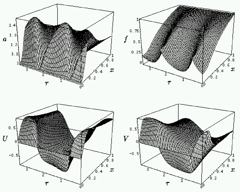
Figure 5: Past patch fields on a single $\Delta$-period.

The error bars in (58) and table 1 are estimated from the convergence properties of the code, which we now explain in detail. In general, we have observed that we can reach higher relative precision in the metric fields than in the matter fields, because the former are essentially integrals of the latter. Figs. 6 and 8 contain all the convergence information for the past patch, but in order to properly discuss convergence issues, we first need to talk about an important feature of the Choptuik spacetime.

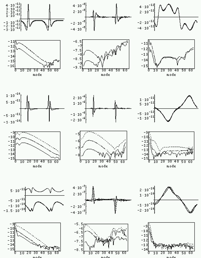
Figure 6: Convergence figures for the past patch. The three columns correspond to $f_{c}$, $\Psi_{c}$ and $U_{p}$, respectively. The six rows are organized in three pairs, describing convergence with respect to ${h_{\rm max}}$, ${x_{\rm left}}$ and ${x_{\rm right}}$ respectively, when these three parameters are halved two or three times. The first row of each pair shows consecutive differences of fields, rescaled by factors 4, 16 and 5.2, respectively, so that they coincide when converging with orders 2, 4 and 2.4, respectively. (Convergence with respect to ${x_{\rm right}}$ is slower than the expected order 3, in particular that of the very low frequency modes of $f_{c}$.) The second row of each pair shows a $\log_{10}$ of the power spectrum of those consecutive differences (without rescaling), to show the different behaviour of the Fourier modes. Convergence of the high frequency modes of $\Psi_{c}$ is worse than that of their low frequency counterparts, as explained in the text.

Fig. 7 shows the field $\Psi(\tau,x)$ together with a log₁₀ plot of the modulus of its Fourier transform in $\tau$. There is a clear difference in behaviour between the regions above and below $x\approx 0.2$. (This difference is present in all our fields, but it is particularly important in $\Psi$, as we will see.) Near the center the function has large $\tau$-derivatives which require many modes in the Fourier expansion to be resolved (see also Fig. 4). Far from the center those derivatives are much smaller and just a few modes are enough to achieve high resolution results. This is reflected in a very slow decay of the Fourier transform near $x\sim x_{c}$ and a fast decay for $x$ above $0.2$, although both are exponential decays. It is important to emphasize that this exponential decay is the best numerical evidence we have in support of the analytical character of the Choptuik spacetime, given the absence of a mathematical proof of existence of an analytical solution to which our numerical spacetime should be converging.

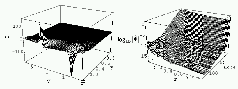
Figure 7: $\Psi(\tau,x)$ and its power spectrum $\left|\hat{\Psi}_{2k+1}(x)\right|$. Note the difference in behaviour between the regions below and above $x\sim 0.2$.

We have observed as well that the phases of the high frequency modes $\hat{Z}_{k}$ tend to a linear dependence on $k$ at a given point $x$. Therefore the high frequency behaviour of our fields $Z$ is similar to that of the function

$$\sum_{k=-\infty}^{\infty}e^{-a|k|}\;e^{\frac{4\pi ik\tau}{\Delta}}=\frac{\sinh a}{\cosh a-\cos\frac{4\pi\tau}{\Delta}},$$ (59)

which has periodic sharp peaks of width $a\Delta/(4\pi)$ and height $2/a$ for small $a$. In the Choptuik spacetime the decay exponent $a$ ranges from $0.28$ for $f_{c}$ at the center to $2.04$ for $U_{p}$ at the past lightcone. We have not found an explanation for this behavior, but it seems to be of dynamical origin: Arbitrary high-frequency perturbations of the correct free data at the center decay towards larger $x$, and high-frequency perturbations at the past lightcone grow when integrated towards the center, probably due to $1/r$ factors in the equations of motion.

From a numerical point of view, this means that aliasing problems will be important near the center $x=0$. This forces us to use a large $N$ ($N=512$ in Fig. 7). But then most of the modes become essentially random for $x\gtrsim 0.2$ because they are well below the error threshold given by roundoff error, estimated in $10^{-14}$ in relative terms. This threshold generates the flat plateau in the right panel of Fig. 7. The main sources of roundoff error are threefold: ODE integration along $x$, Fourier transforms, and inversion of a very stiff matrix in Newton’s method. Particularly important are the errors in the modes of $U_{p}$ above $k=15$ because they propagate inwards and get amplified, giving errors of relative order $10^{-9}$ in the matter fields, mainly in $\Psi_{c}$. (See Fig. 7 again.) This fact sets the limit of the maximum accuracy that we can get in the results, with just double precision numerics and using our code. We could use quadruple precision to improve the precision in $U_{p}$ but the calculations would become too slow. Alternatively, we could force the vanishing of those modes that we believe must vanish, but we do not want to assume anything at all about the result in advance.

We now check convergence with respect to the numerical parameters. As one would expect, the final solution is completely insensitive to the choice of intermediate fitting point ${x_{\rm mid}}$, although the convergence of Newton’s method is faster when using smaller values because the mismatches are larger. We choose ${x_{\rm mid}}=0.01$.

Several tests in simpler problems show that the ODE integrator in $x$ is perfectly fourth-order convergent. The first two rows of figure 6 also show this fact, even though roundoff errors slightly blur the point. Note that the modes of $U_{p}(\tau)$, after the first 10, do not converge because they are already below our error threshold (on the plateau in Fig. 7). Note also that high-frequency modes of $\Psi_{c}$ do not converge for such small values of ${h_{\rm max}}$. They do converge for larger values.

Convergence with $N$ is exponential as expected. Fig. 8 shows the power spectra of the free data for $N=32,64,128,256,512$. It clearly shows how much the results are improved by doubling $N$ and how the plateau goes down each time, until $N=256$, when errors in $U_{p}$ hit our error threshold. The data for $N=512$ shows that we cannot improve the results any further because we cannot decrease the errors in $U_{p}$. $f_{c}$ is then perfectly resolved down to machine precision, but high-frequencies of the matter variables cannot be improved near the center. It is clear that using $N=256$ or $N=512$ we are not affected by aliasing errors.

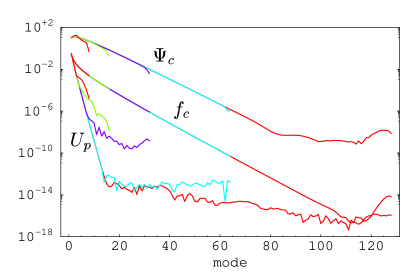
Figure 8: Power spectra of the free data for 8, 16, 32, 64 and 128 modes. Note the very different behaviors of the functions $f_{c}$ and $\Psi_{c}$ at the center from the function $U_{p}$ at the past lightcone.

Finally, convergence with ${x_{\rm left}}$ and ${x_{\rm right}}$ depends on the value of $N$: As we said, we calculate the fields at ${x_{\rm left}}$ and ${x_{\rm right}}$ using Taylor expansions:

$$f(\tau,x) = f_{c}(\tau)+f_{2}(\tau)(x-x_{c})^{2}+O\left[(x-x_{c})^{4}\right],$$ (60)

$$U(\tau,x) = U_{p}(\tau)+U_{1}(\tau)(x-x_{p})$$ (61)

$$+U_{2}(\tau)(x-x_{p})^{2}+O\left[(x-x_{p})^{3}\right],$$

and so for the other fields. Therefore we expect fourth order convergence with respect to ${x_{\rm left}}$ and third order with respect to ${x_{\rm right}}$. The coefficients of the Taylor expansions are obtained as nonlinear combinations of the free data and their $\tau$-derivatives. The latter are calculated multiplying the Fourier modes $\hat{Z}_{k}$ by $ik$, which amplifies the high frequency modes. Fig. 9 shows the Fourier transforms of $\Psi_{c},\Psi_{2},\Psi_{4}$ obtained for different values of $N$. For low $N$ our estimations of these coefficients are bad and we do not see the expected convergence order in the expansions with ${x_{\rm left}}$ and ${x_{\rm right}}$, both because we are cutting off too soon in frequency, leaving out modes which are important (see for instance the case of $\Psi_{2}$ with $N=64$), and because of aliasing errors, which gives us wrong estimations of the modes that we are including (see the unphysical tails at the end of the functions). The same phenomenon happens on the past lightcone, but its effect is not so important. That is the main reason why we need at least $N=256$ to get good results. However, for higher $N$ we do see clear convergence with the expected orders (with the exception of the very low $k$ modes, whose convergence with respect to ${x_{\rm right}}$ is slower due to accumulation of high-frequency errors in $U_{p}$). This is shown in Fig. 6.

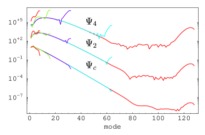
Figure 9: Power spectra of the functions $\Psi_{c}$, $\Psi_{2}$ and $\Psi_{4}$ for 8, 16, 32, 64 and 128 modes. Aliasing problems show up as unphysically growing tails for the highest frequencies in each case. Working with only 32 modes, this introduces errors in $\Psi_{2}$ which are of the same order of the amplitude of the most important modes. We cannot avoid going to at least 64 modes (that is, $N=256$). $\Psi_{4}$ is presented for illustration purposes only; we do not use it in the code.

We conclude that the code converges in the expected manner with respect to all numerical parameters. Therefore we can estimate the error of the base run (57) with respect to any of the parameters of the code as the difference between the base run and another run with a refined value of that parameter. Those are precisely the continuous lines in Fig. 6. Truncation errors from space and time discretization could be reduced to machine precision. However, errors from the expansions at the singular points cannot be brought down with our code below a limit which we estimate (assuming no systematic error) between $10^{-8}$ and $10^{-9}$ in relative terms. Therefore there is no point in reducing the other sources of error below that limit, and the choice of parameters for our base run (57) reflects this.

IV.3 Outer patch

In the entire outer patch the fields are much smoother in $\tau$ (as they are already on the past patch for $x\gtrsim 0.2$). Therefore we only need a few Fourier modes to get good precision. In fact $N=64$ is enough to reach the maximum accuracy given by propagation of the errors in the past patch. There is no reason to increase $N$ further.

Table 2: The first 8 nontrivial Fourier modes of the outer patch free data. (The error in the last digit is shown in brackets.) Note the very different relative precisions achieved in $\xi$ and $\hat{U}_{\epsilon}$. The former is insensitive to changes in the parameters of the code, but not the latter.

$k$	Re $\hat{\xi}_{2k}$	Im $\hat{\xi}_{2k}$	Re $\hat{V}_{2k+1}(x_{f})$	Im $\hat{V}_{2k+1}(x_{f})$	Re $\hat{\hat{U}}_{\epsilon}{}_{2k+1}$	Im $\hat{\hat{U}}_{\epsilon}{}_{2k+1}$
0	1.322045988(6)	0	-5.177664(12)$\cdot 10^{-4}$	3.157186(5)$\cdot 10^{-4}$	-0.03844(5)	-0.250325(8)
1	-0.00492853319(12)	-0.00430580184(14)	-1.5(3)$\cdot 10^{-10}$	-2.0(7) $\cdot 10^{-10}$	0.003883(8)	-0.0121478(20)
2	-1.1237092(5) $\cdot 10^{-5}$	2.89549492(5)$\cdot 10^{-4}$	-1.(4) $\cdot 10^{-12}$	2.(15) $\cdot 10^{-13}$	2.895(8)$\cdot 10^{-4}$	-5.853(3)$\cdot 10^{-4}$
3	1.99072448(4)$\cdot 10^{-5}$	-6.20831744(26) $\cdot 10^{-6}$	-1.(5) $\cdot 10^{-13}$	0.(31) $\cdot 10^{-14}$	1.748(5) $\cdot 10^{-5}$	-2.5842(28) $\cdot 10^{-5}$
4	-1.078319002(12)$\cdot 10^{-6}$	-1.46908361(3) $\cdot 10^{-6}$	1.(30) $\cdot 10^{-14}$	-1.(6) $\cdot 10^{-13}$	8.957(26) $\cdot 10^{-7}$	-1.0219(20) $\cdot 10^{-6}$
5	-1.032893598(26) $\cdot 10^{-7}$	1.436706184(10) $\cdot 10^{-7}$	-0.(21) $\cdot 10^{-14}$	0.(4) $\cdot 10^{-13}$	4.126(10) $\cdot 10^{-8}$	-3.920(10) $\cdot 10^{-8}$
6	1.74888526(8) $\cdot 10^{-8}$	5.7084263(10) $\cdot 10^{-9}$	1.(25) $\cdot 10^{-14}$	0.(4) $\cdot 10^{-13}$	1.826(4) $\cdot 10^{-9}$	-1.454(4) $\cdot 10^{-9}$
7	2.39356(8) $\cdot 10^{-11}$	-2.0053466(8) $\cdot 10^{-9}$	0.(3) $\cdot 10^{-13}$	0.(3) $\cdot 10^{-14}$	7.79(12) $\cdot 10^{-11}$	-5.21(26) $\cdot 10^{-11}$

With $x_{p}=-1$ and $x_{f}=1$ we choose these parameters for the numerical evolution:

$$N = 64,$$

$${x_{\rm left}} = -0.9999,$$

$${x_{\rm mid}} = -0.9,$$ (62)

$${x_{\rm right}} = 0.9999,$$

$${h_{\rm max}} = 0.001,$$

Now the free data are the metric function $\xi(\tau)$ and the matter functions $V_{f}(\tau)\equiv V(\tau,x_{f})$ and $\hat{U}_{\epsilon}(\tau)$ at the future lightcone. (Note that the function $V_{f}$ was called $V_{0}$ in Subsection III.3.)The results are given in table 2 and Fig. 10, with a final value

$$\epsilon=1.4710439(8)\cdot 10^{-6},$$ (63)

clearly different from zero. We firmly believe that this is neither a numerical artifact nor a consequence of our expansion around the future lightcone. After showing convergence of the code in the outer patch, we dedicate most of this subsection to supporting this claim.

Figure 10: Free data in the outer patch: 20$V_{f}$ (continuous line), $\hat{U}_{\epsilon}/20$ (dotted line) and $\xi-1.3$ (dash-dotted line). Note that they are all quite smooth.

The integrated functions are shown in Fig. 11. The runaway of characteristics is not apparent in this figure, because all but the first oscillations are piled up in the region between $x=0.95$ and $x=1$. Fig. 12 shows $U$ using a logarithmic $x$-axis.

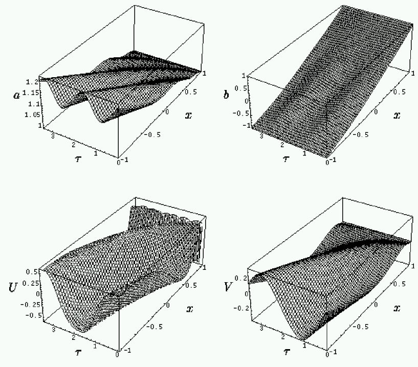
Figure 11: Outer patch fields on a single $\Delta$-period.

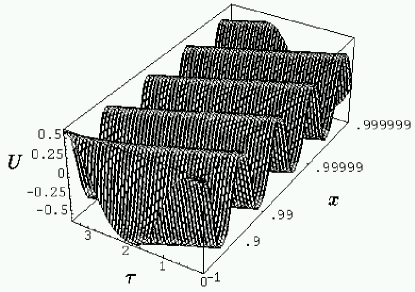
Figure 12: $U$ in the outer patch using a logarithmic $x$-axis. The oscillations are clear, but not their slow decay.

We first analyze the issue of error propagation from the past patch to the outer patch. We need to find out how small variations in $\Delta$ and $U_{p}$ change the results of the outer patch shooting. Assuming that the former are small, we calculate first derivatives of the latter. The variations of the outer patch free data with respect to $\Delta$ are:

$$\frac{\delta\epsilon}{\delta\Delta}=5.4\cdot 10^{-6}, \frac{||\delta V_{f}||_{\infty}}{\delta\Delta}=0.0020,$$ (64)

$$\frac{||\delta\hat{U}_{\epsilon}||_{\infty}}{\delta\Delta}=0.15, \frac{||\delta\xi||_{\infty}}{\delta\Delta}=0.028.$$ (65)

On the other hand, Fig. 13 shows the maximum variations of the free data with respect to changes of the Fourier modes of $U_{p}$. We see that $V_{f}$ and $\xi$ are only sensitive to the very low frequency modes of $U_{p}$, but $\hat{U}_{\epsilon}$ changes with every mode. In any case, every derivative is small enough: The largest error bars come from the uncertainty in $\Delta$, and then from those of the first two modes in $U_{p}$. The rest of the modes are practically irrelevant for error analysis. This sets the maximum accuracy that we can achieve on our final results. Assuming quadratic error propagation it is

$$\delta_{\rm max}\epsilon = 5\cdot 10^{-13},$$ (66)

$$||\delta_{\rm max}V_{f}||_{\infty} = 2\cdot 10^{-9},$$ (67)

$$||\delta_{\rm max}\hat{U}_{\epsilon}||_{\infty} = 4\cdot 10^{-8},$$ (68)

$$||\delta_{\rm max}\xi||_{\infty} = 2\cdot 10^{-8}.$$ (69)

It is still very good due to the tendency of small perturbations to decay when integrating towards larger $x$, and, as we said, achievable already with $N=64$.

Figure 13: Variation of the results of the outer patch under changes of the input data from the past patch. On the left we represent $||\delta f||_{\infty}/\delta p_{k}$ where $\delta f$ is the change in $10^{5}\epsilon$ (continuous line) or in one of the functions $10^{2}V_{f}$ (dotted line), $\xi$ (dashed line) or $\hat{U}_{\epsilon}$ (dot-dashed line), under a change $\delta p_{k}$ in the real part of the mode $k$ of $U_{p}$. On the right we show the same for the imaginary part of the modes of $U_{p}$. We lack enough precision to calculate the last point of the $V_{f}$ curves.

We now analyze convergence in the outer patch. Convergence with ${h_{\rm max}}$ in the IRK2 method shows perfect fourth order again. Convergence with ${x_{\rm left}}$ is approximately third order as expected because we expand around the past lightcone with a second-order Taylor series. See Fig. 14. Finally, we have performed calculations expanding around $x_{f}$ using only the order zero terms and including the first order terms.

$V_{f}$ and $\xi$ converge with ${x_{\rm right}}$ to first order when the expansion around the CH is truncated at $O(|y|^{\epsilon})$, and converge to second order when the expansion is truncated at $O(|y|^{1+3\epsilon})$. This is the expected behavior. However, at the same time $\hat{U}_{\epsilon}$ converges to first order in both cases (see Fig. 14). This indicates that adding the terms of order $O(|y|^{1+k\epsilon})$ (with $k=0,1,2,3$) to the expansion still leaves some $O(|y|^{1+k\epsilon})$ error. We are confident that this is not a simple algebraic mistake in the expansion. We note that the excess error in the periodic function $\hat{U}_{\epsilon}$ is entirely an error in its overall phase. We therefore suspect intuitively that the runaway phase $U\sim\hat{U}_{\epsilon}(\tau-\ln|y|)$ of the solution is to blame, but we have not been able to formulate this idea consistently.

Figure 14: Convergence of the free data on the outer patch. These plots display norms of differences between consecutive results: $\infty$-norm (continuous line) and 2-norm (dotted line). On the left, convergence with respect to ${x_{\rm left}}$ shows order 3.0 for $\hat{U}_{\epsilon}$ (triangles) and $\xi$ (diamonds) and order 2.4 for $V_{f}$ (stars). On the right, convergence with respect to ${x_{\rm right}}$ shows order 2.0 for $\xi$ and $V_{f}$ and order 1.0 for $\hat{U}_{\epsilon}$.

In order to show that $\epsilon$ is really different from zero, we have to analyze the behavior of the function $V$ with respect to ${x_{\rm left}}$ and ${x_{\rm right}}$. The function $V_{f}$ has a very rapidly decaying Fourier spectrum, as shown in Fig. 15. As $x_{\rm left}\to x_{p}$, all its Fourier modes converge to zero except for the first two, and the amplitude of the second mode is more than six orders of magnitud below that of the first one (see also Table 2).

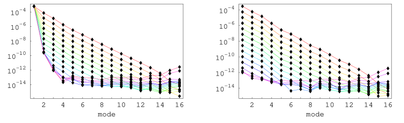
Figure 15: Convergence of $V_{f}$. Left figure: $\log_{10}|\hat{V}_{f}{}_{2k-1}|$ for 15 values ${x_{\rm left}}=$-0.8976, -0.9488, -0.9744, -0.9872, -0.9936, -0.9968, -0.9984, -0.9992, -0.9996, -0.9998, -0.9999, -0.99995, -0.999975, -0.9999875, corresponding from top to bottom, respectively. It seems that all but the first two modes converge to amplitudes below our error threshold when ${x_{\rm left}}$ approaches -1, even though high-frequencies become unstable for the last values of ${x_{\rm left}}$. Right figure: modulus of the Fourier transform of consecutive differences in the left figure. Convergence is very clear in every mode (including the first one).

Fig. 16 shows $\overline{V^{2}}(x)$ for several evolutions from the same ${x_{\rm left}}=-0.9999$ to 15 different values of ${x_{\rm right}}$. The agreement is very good. This shows that our expansion around the future lightcone (including the singular terms given in the appendix) captures the behavior of the solution.

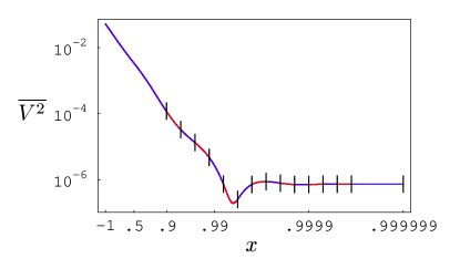
Figure 16: Average of $V^{2}$ on $\tau$ for different evolutions from the same ${x_{\rm left}}=-0.9999$ to 15 different values of ${x_{\rm right}}$ (those of table 3). The agreement between the solutions with small ${x_{\rm right}}$ and those with ${x_{\rm right}}$ very close to $x_{f}=1$ implies that the final almost constant value is neither a numerical artifact nor a consequence of our ansatz.

We conclude that, with errors of order $10^{-9}$,

$$V_{f}(\tau)=-1.2128648(22)\cdot 10^{-3}\cdot\cos\left(\frac{2\pi\tau}{\Delta}+0.5475726(13)\right).$$ (70)

Table 3: Convergence of $10^{6}\epsilon$ with ${x_{\rm right}}$ using only the lowest order terms in the regular expansion plus only the $O(y^{\epsilon})$ in U (first column) and using the full next order as well (second column). Convergence is much faster in the second case, as expected, but it is clear that both converge to the same number, within our error bars. Recall that digits starting from the fifth decimal are not relevant due to propagation of errors from the past patch. They are shown in the second column to make convergence clear.

${x_{\rm right}}$	zeroth order	first order
0.8976	238.46	0.87085
0.9488	66.166	1.36313
0.9744	26.743	1.49818
0.9872	9.4840	1.48105
0.9936	1.4699	1.47058
0.9968	0.5058	1.470305
0.9984	1.4386	1.470949
0.9992	1.7639	1.4710727
0.9996	1.5837	1.4710534
0.9998	1.4355	1.47104333
0.9999	1.4332	1.47104318
0.99995	1.4687	1.471043825
0.999975	1.4799	1.471043941
0.9999875	1.4743	1.471043921
0.999999	1.4713	1.471043911

Finally, it is interesting to see that going to $O(|y|^{1+3\epsilon})$ is not essential for obtaining an accurate result. Table 3 compares the results for $\epsilon$ using a zeroth-order expansion (that is, we only include the terms of orders $y^{0}$ and $|y|^{\epsilon}$) with those from the first order expansion (which also includes orders $y$ and $|y|^{1+k\epsilon}$). It is clear that they both converge to the same number, even though with very different rates of convergence.

V Continuation across the Cauchy horizon: the future patch

V.1 The continuation with a regular center

We cannot continue the solution as flat empty Minkowski spacetime after the Cauchy horizon because we have a small amount of ingoing radiation there, given by $V_{f}(\tau)$. The simplest continuation to look for is one with a regular timelike center, so that the conformal diagram is the same as for Minkowski spacetime. In this case both $U$ and $V$ are small on the entire future patch, and we can obtain an approximate solution in perturbation theory around Minkowski space, using the magnitude $\epsilon^{1/2}$ of $V_{f}$ as the small parameter. To leading order in $\epsilon$ we obtain the d’Alembert solution on flat spacetime:

$$f = 1+O(\epsilon),$$ (71)

$$a = 1+O(\epsilon),$$ (72)

$$U = \epsilon^{1/2}\left[-F^{\prime}(\hat{\tau})-\frac{F(\hat{\tau})+G(\tau)}{x}\right]+O(\epsilon^{3/2}),$$ (73)

$$V = \epsilon^{1/2}\left[-G^{\prime}(\tau)+(1+x)\frac{F(\hat{\tau})+G(\tau)}{x}\right]+O(\epsilon^{3/2}),$$ (74)

with $\hat{\tau}\equiv\tau-\ln(1+x)$. In order to match the null data on the Cauchy horizon $x=-1$, we need $-\epsilon^{1/2}G^{\prime}(\tau)=V_{f}(\tau)$. Recall that $V_{f}(\tau)$ is given numerically by (70). If we want to have a regular solution at the center we need $F(\tau)=-G(\tau)$. The solution is then completely determined, and it is clear that a nonlinear solution exists of which this is the leading order, and which can be found numerically.

Because the null data $V_{f}$ on the Cauchy horizon are DSS, it appears highly unlikely that there is another continuation with a regular timelike center that is not DSS. We have obtained the (probably) unique regular continuation by shooting from expansions around the Cauchy horizon and a regular center. The free data for the shooting algorithm (given by $\hat{U}_{\epsilon}$ at the CH and $f$, $U_{,x}$ at the center) were obtained from the flat spacetime approximation. In this case we use an IRK1 integrator and

$$N = 16,$$

$${x_{\rm left}} = -0.999,$$

$${x_{\rm mid}} = -0.2,$$ (75)

$${x_{\rm right}} = -0.001,$$

$${h_{\rm max}} = 2.5\cdot 10^{-4},$$

with very good convergence, that we do not show again. The fields $a$, $f$, $U$ and $V$ are shown in Fig. 17.

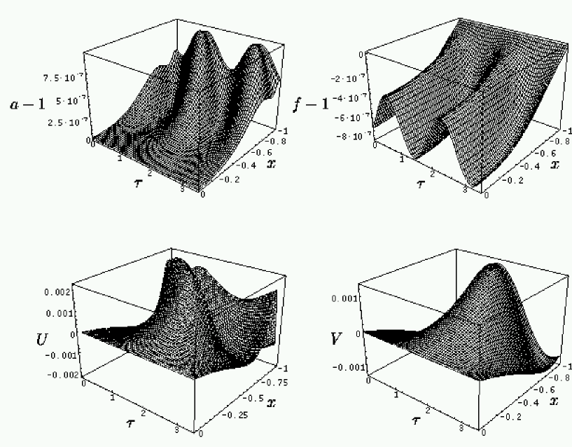
Figure 17: Future patch fields on a single $\Delta$-period for the (probably unique) continuation with a regular timelike center. Note that $a$ and $f$ are so close to their flat spacetime values that we plot their difference from 1, rather than the fields themselves.

V.2 All other continuations

We now consider the other possible continuations, in particular those of Figs. 2 and 3. Before performing a numerical search of the possibilities in the $\hat{U}_{\epsilon}$ space, we study the equations of motion in the future patch. We proceed in four steps:

A necessary condition for another SSH is $a^{2}>2$.

In order to obtain Fig. 3, or any even more exotic continuation, we must have a self-similarity horizon before the central singularity occurs at $x=x_{s}=0$.

A self-similarity horizon is a DSS line $x=x_{h}(\tau)$ (periodic) where $A=0$. The only factor in $A=-4a^{2}f(f+x)$ that can vanish (while the metric is regular) is $f+x$. We have

$$(f+x)_{,x}=\frac{(a^{2}-1)f}{x}+1$$ (76)

and so

$$\left.(f+x)_{,x}\right|_{f+x=0}=2-a^{2}.$$ (77)

At the Cauchy horizon $f+x=0$ and $(f+x)_{,x}\simeq 1$ because $a^{2}-1$ is small, and so $(f+x)>0$ and $A<0$ at least to the immediate future of the Cauchy horizon. If there are more self-similarity horizons to the future of the Cauchy horizon, we must have $f+x=0$ again there, and therefore $(f+x)_{,x}<0$ in some intermediate region. $a^{2}$ must increase from $a^{2}\simeq 1$ to $a^{2}>2$ in order to achieve this.

Once $a^{2}<1$ for any $\tau$, $a^{2}\to 0$ for that $\tau$.

$a$ is given by the constraint (52) which reduces at the Cauchy horizon to

$$(a^{-2})_{,\tau}=(1+2V_{f}^{2})a^{-2}-1,$$ (78)

and this means that $1<a<1+\epsilon$ there. Now $a$ obeys the evolution equation

$$-2x(\ln a)_{,x}=a^{2}-1-2U^{2}.$$ (79)

Recall that in the future patch $x<0$ and increases towards the future. Therefore $a=1$ is a repeller in the absence of matter, but any outgoing radiation $U$ drives $a$ to smaller values. Hence, once $a$ becomes smaller than 1 for some value of $\tau$, it will afterwards decrease to 0 for that $\tau$ whatever happens. Because $\mu=2m/r=1-a^{-2}$, this means that we are in a negative mass regime and remain there until we reach the central singularity $x=0$, which is therefore timelike and has negative infinite mass at least for this $\tau$. The singularity cannot be reached with a finite value of $0<a^{2}<1$.

Is $a^{2}>1$ at the singularity possible at least for some values of $\tau$?

If we choose $\hat{U}_{\epsilon}$ much larger than $O(\epsilon^{1/2})$, the $U^{2}$ term will drive $a$ to $a<1$ almost immediately. However, we know that the regular solution does not have negative mass and therefore it seems plausible that functions $\hat{U}_{\epsilon}$ close to the regular case could generate a singularity with positive mass. We shall now argue that this is not true.

$a$ can only increase from its CH value if $|\hat{U}_{\epsilon}|$ is very small. In order to explore this regime we return to the approximation of perturbing around Minkowski spacetime, but now dropping the assumption that $F(\tau)=-G(\tau)$. The result can be summarized as:

$$a(\tau,x) = 1+\epsilon\;x^{2}a_{\rm reg}(\tau,x)$$

$$- \epsilon\;x^{-2}\left[F(\tau)+G(\tau)\right]^{2}$$

$$+ \epsilon\;O(x^{-1})+O(\epsilon^{3/2}).$$

The function $a_{\rm reg}$ is positive and always smaller than 2, and is independent of $F$. All singular terms vanish for $F=-G$. For every other $F$, the function $a$ becomes smaller than 1, which corresponds to negative mass, as the center $x=0$ is approached. This is due to the divergent terms $(F+G)/x$ in (73) and (74). The crucial point is that $a^{2}$ is integrated from $-U^{2}$ and therefore the term in the perturbation expansion that makes the mass nonzero has coefficient $-(F+G)^{2}$, and so the mass cannot be positive. The negative mass regime is reached while perturbation theory still applies, and we have seen that afterwards the mass must decrease indefinitely.

With these arguments we have ruled out the possibility of having positive mass at the singularity for very large $\hat{U}_{\epsilon}$ and for very small (in particular, close to the regular case) $\hat{U}_{\epsilon}$. However we could be missing some intermediate regime where perturbation theory does not apply. For these intermediate cases we observe that the minimum of $a$ is far from 1 (and therefore we cannot apply perturbation theory), but its maximum is positive and close to 1, and only becomes negative in the vicinity of the singularity. There could be solutions where $a$ is positive at the singularity for some values of $\tau$.

Numerically, however, we do not find that. We have performed a large number of numerical evolutions in this intermediate regime starting from $\hat{U}_{\epsilon}=2^{n}\,\hat{U}_{\epsilon}{}_{\rm reg}(\tau+m\Delta/8)$, for $n=-5,...,10$ and $m=0,...,7$. Even though it is difficult to evolve the system near the singularity, we always observe a final decay of $a$ to 0. See Fig. 18. Therefore we believe that, starting from small null data $V_{f}$ at the CH it is not possible to form another SSH. Therefore, either we have a regular center or a timelike singularity, and this singularity always has negative mass. In the approach to the center with $a^{2}\to 0$ we always have $U+V\to 0$ with both $U,V$ finite. It should be stressed that this scenario is a consequence of the small amplitude of the null data $V_{f}$ on the Cauchy horizon in the Choptuik solution. We have performed other evolutions starting from large null data on the Cauchy horizon (not $V_{f}$ of the Choptuik solution) where $a^{2}$ increases beyond 2.

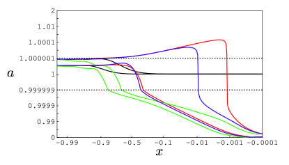
Figure 18: Maximum and minimum of $a$ for different initial data functions $\hat{U}_{\epsilon}$ from numerical evolutions of the nonlinear equations. Note that the $x$ axis becomes logarithmic when approaching the boundaries, while the $a$ axis is linear between the dotted lines at $a=1-10^{-6}$, $a=1+10^{-6}$, and logarithmic elsewhere. The initial $\hat{U}_{\epsilon}$ have been obtained multiplying the regular data (black) by different constants: 0 (red), -1 (blue) and 5 (green). Clearly, the larger $\hat{U}_{\epsilon}$ is, the sooner $a$ decays.

How is the singularity approached?

We find that in all numerical continuations $a\to 0$, $f\to\infty$, $U$ and $V$ tend to finite values and $U\to-V$ as the singularity $x=0$ is approached. If we assume that $a\to 0$ and $U\to U_{0}(\tau)$ as $x\to 0$ then the $a_{,x}$ and $f_{,x}$ equations to leading order give

$$f \simeq f_{0}(\tau)\,x^{-1},$$ (81)

$$a^{2} \simeq a_{0}^{2}(\tau)\,|x|^{2\alpha(\tau)},\qquad\alpha(\tau)\equiv\frac{1}{2}+U_{0}(\tau)^{2}.$$ (82)

Making the ansatz that

$$U \simeq U_{0}(\tau)+U_{2}(\tau)\,x^{2}$$ (83)

$$+\,U_{2l}(\tau)\,x^{2}\ln|x|+U_{\alpha}(\tau)\,|x|^{2\alpha(\tau)},$$

$$V \simeq V_{0}(\tau)+V_{2}(\tau)\,x^{2}$$ (84)

$$+\,V_{2l}(\tau)\,x^{2}\ln|x|+V_{\alpha}(\tau)\,|x|^{2\alpha(\tau)},$$

we find from the $U_{,x}$ and $V_{,x}$ equations to the leading order, $O(\ln|x|)$ that

$$V_{0} = -U_{0},$$ (85)

$$V_{2} = U_{2}+{1\over 2}f_{0}^{-1}U_{0}^{\prime},$$ (86)

$$U_{2l}=V_{2l} = -\frac{1}{2}f_{0}^{-1}U_{0}^{\prime},$$ (87)

$$U_{\alpha}=-V_{\alpha} = -\frac{1}{2\alpha}a_{0}^{2}U_{0}.$$ (88)

(The expansion also holds in the special case $\alpha=1$.) The next order, $O(1)$, gives

$$\ln(a_{0}^{2})^{\prime}+1+2U_{0}^{2}+8f_{0}U_{0}U_{2}+2U_{0}U_{0}^{\prime}=0.$$ (89)

The metric in the future patch contains a residual gauge freedom worth one periodic function of $\tau$. Near the singularity $x=0$, we can fix this gauge freedom by setting $f_{0}(\tau)$ to an arbitrary value. (In our numerical evolutions starting at the Cauchy horizon, the gauge has of course been fixed already by setting $f=1$ at the Cauchy horizon.) $U_{0}(\tau)$ and $U_{2}(\tau)$ are then physical free data which determine $a_{0}(\tau)$ and all other coefficients of the expansion. (Eq. (89) can be solved for $a_{0}$ only if the right-hand side has vanishing average, which means that $f_{0}$ cannot be set completely freely.) This expansion is therefore generic in the sense of depending on two free functions after the gauge has been fixed.

The behavior just described is what we observe numerically for large values of the free data $\hat{U}_{\epsilon}(\tau)$ at the Cauchy horizon. For small values of $\hat{U}_{\epsilon}(\tau)$ we find $U_{0}(\tau)\simeq\pm 1/\sqrt{2}$, that is $\alpha(\tau)\simeq 1$. Note that by our ansatz of exact DSS with $\kappa=0$, $U$ must be an odd function of $\tau$ with zero average. We observe in fact that $U(\tau,x)$ goes to a fundamental frequency square wave of amplitude $1/\sqrt{2}$, that is, in half of each $\tau$-period $U\to 1/\sqrt{2}$, and $U\to-1/\sqrt{2}$ in the other half. This is shown in Fig. 19.

As the center $x=0$ is approached with $U_{0}=\pm 1/\sqrt{2}$, we observe empirically that the $\tau$-derivatives become dynamically negligible. This means that different values of $\tau$ effectively decouple, that at each point $\tau$ the evolution equations become an ODE system in $x$, while the constraint becomes algebraic, and that the spacetime becomes locally CSS. It also means that the evolution equations become “velocity-dominated” in the sense that all derivatives transversal to the singularity (here in spherical symmetry, this is only the $\tau$-derivative) become dynamically irrelevant compared to the one derivative running into the singularity (here, the $x$-derivative). It is known that generic spacelike singularities in general relativity with massless scalar field matter are velocity-dominated AnderssonRendall . Here we find this to be the case only in the limit of small data $\hat{U}_{\epsilon}(\tau)$.

As this class of continuations seems to be locally CSS near the singularity, it is interesting to study the exactly CSS solutions from the point of view of a DSS ansatz. Starting from a generic DSS scalar field (12) we introduce a new (gauge-dependent) variable

$$W\equiv U+\frac{f}{x}(U+V)=\sqrt{2\pi G}(\kappa+\psi_{,\tau}),$$ (90)

which coincides with $-V$ at the future lightcone $f/x=-1$, and obeys the equation

$$xW_{,x}=-U_{,\tau}.$$ (91)

In exactly CSS solutions of the system the metric functions and $U,V$ are independent of $\tau$, and hence $W$ is constant with value $W=\sqrt{2\pi G}\kappa$. The CSS solution with $\kappa=0$ was found in closed form by Roberts Roberts and is described in Appendix C. The CSS solutions with $\kappa\neq 0$ were studied numerically by Brady Brady .

We find that the small $\hat{U}_{\epsilon}(\tau)$ continuations locally approach a Roberts solution (with $\kappa=0$) with a value of the parameter $p$ of the Roberts solution that depends on $\tau$, and not, as one might have expected, one of Brady’s solutions. This is discussed in Appendix C.

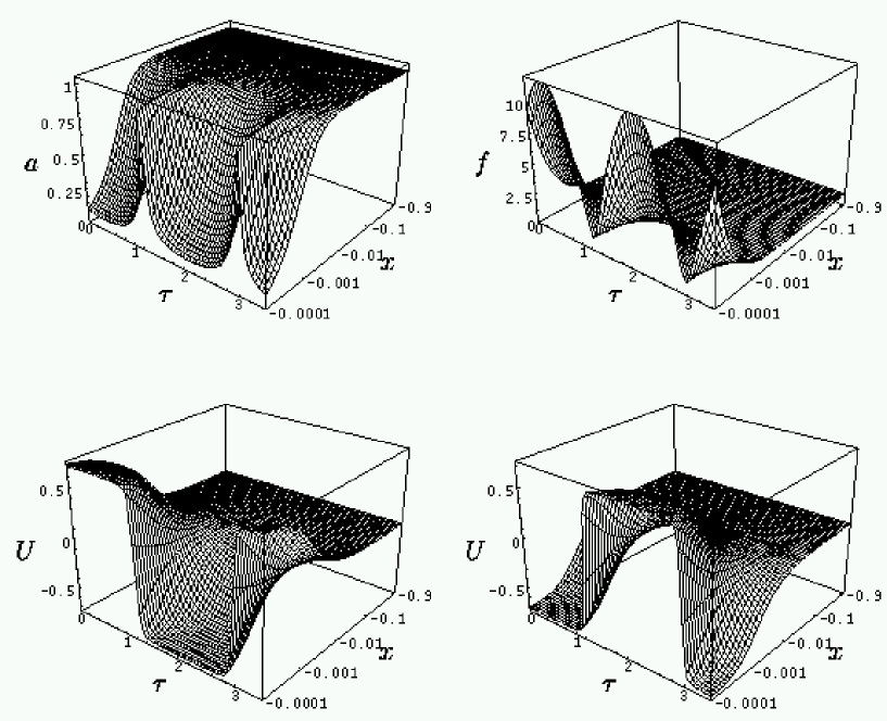
Figure 19: Future patch fields on a single $\Delta$-period for a singular continuation of the Choptuik spacetime.

VI Global images of the Choptuik spacetime

Figures 5, 11, 17 and 19 show in a very detailed way the structure of the Choptuik spacetime. However it is difficult to get from them an idea of what it looks like globally. In this final Section before the conclusions we present a number of additional figures that will fill this gap. We do it in two very different ways.

VI.1 Global coordinate systems

As shown in Fig. 1, our three $(\tau,x)$ patches match continuously, but we do not expect the resulting global coordinate system to be differentiable at the interfaces between the patches. The critical spacetime itself, however, is differentiable (analytic at the past lightcone and $C^{1}$ at the CH), and it must be possible to construct global coordinate systems which are at least $C^{2}$.

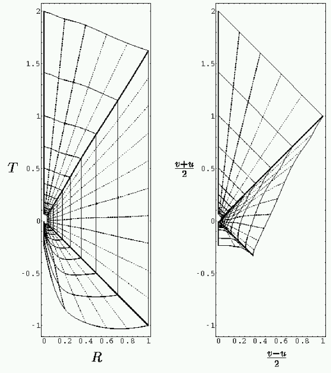
Figure 20: Spacetime diagrams for a single period of the Choptuik spacetime in differentiable coordinate systems (synchronous-area on the left and double null on the right). It is possible to construct the whole spacetime by adding rescaled (by a factor $e^{\Delta}=31.357$ or its inverse) blocks to the center and outside the figures. Continuous lines represent $\tau=const.$ lines and dashed lines represent $x=const.$ lines. By our gauge choices times $T$ and $(v+u)/2$ coincide on the centre worldline.

One simple possibility is synchronous slicing plus area gauge:

$$ds^{2}=-dT^{2}+2B(T,R)dTdR+C(T,R)dR^{2}+R^{2}d\Omega^{2}.$$ (92)

We add the gauge condition $T=-R$ on the past lightcone of the singularity. The coordinate transformation $T(\tau,x),R(\tau,x)$ can be easily integrated and it is shown on the left panel of Fig. 20 for a single $\Delta$-period in $\tau$.

Another simple possibility is double null coordinates:

$$ds^{2}=-\omega(u,v)dudv+R^{2}(u,v)d\Omega^{2}$$ (93)

with gauge condition $u=v=T$ at the center, where $T$ is the time coordinate constructed in the previous paragraph. The coordinate change $u(\tau,x),v(\tau,x)$ is shown on the right panel of Fig. 20 for a single $\Delta$-period in $\tau$.

The fields $a$, $U$ and $V$ in double null coordinates are shown in Fig. 21. As these fields are spacetime scalars, they should be analytic in these coordinates at the past lightcone, and $C^{1}$ at the Cauchy horizon. In the plot it looks as if they are only $C^{0}$ at the Cauchy horizon, but that is due to a lack of resolution in the plot: the slopes on the two sides of the Cauchy horizon are dominated by $a_{1+\epsilon}$ and $a_{1+2\epsilon}$, which are discontinuous at the resolution of the plot, but close enough to the Cauchy horizon, the slope becomes $a_{1}$, which is continuous.

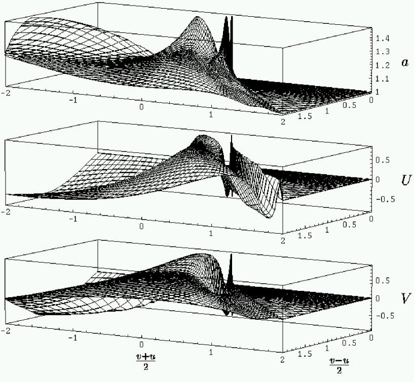
Figure 21: Scalars $a$, $U$ and $V$ as functions of the double null variables $u$ and $v$. Grid lines are lines of constant $x$ or $\tau$. Time is increasing from left to right, and the central world line is at the back.

VI.2 Dynamical phase space portraits

We shall now consider the spherical DSS scalar field as an infinite-dimensional dynamical system where $x$ is the “time” coordinate. The dynamical variables in this system are $U(\tau)$, $V(\tau)$ and $f(\tau)$ (or $b(\tau)$ in the outer patch). The variable $a(\tau)$ is not independent, but given by a constraint. However, many solutions of the dynamical system correspond to the same spacetime, namely all that are related by the coordinate transformations (5). The pair of periodic functions $U(\tau)$ and $V(\tau)$ describes a closed, possibly self-intersecting curve in the $(U,V)$ plane. An entire evolution in $x$ gives a surface that is topologically a cylinder, which we may call a phase portrait of the solution. Clearly the surface itself is invariant under the coordinate change $\tau\to\tau+\psi(x,\tau)$. If we consider $\tau$ as our “space” coordinate in the usual “3+1” split, then by looking at the phase portrait we have eliminated the “spatial” gauge freedom. The “slicing” freedom $x\to\varphi(x,\tau)$ however does change the shape of the phase portrait, so it is not completely gauge-invariant. The Choptuik spacetime up to the CH is given in Fig. 22 and its regular continuation is shown in Fig. 23.

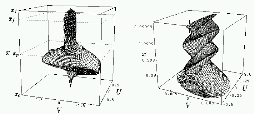
Figure 22: Left: Phase-portrait of the Choptuik spacetime from the regular past centre at $x_{c}$ to the CH at $x_{f}$. The $x$-axis has been highly distorted in order to show all interesting details: the axis is logarithmic between $x_{c}$ and $x_{p}$ with accumulation point at $x_{c}$ (note that the label $x_{c}$ has been situated at finite distance for convenience); the axis is logarithmic with accumulation at $x_{f}$ between $x_{p}$ and $\bar{x}_{f}$; the axis has been transformed from $x$ to $x_{f}-x^{1/\epsilon}$ to show the decay of the function $U$ towards $x_{f}$ (this is a semi-analytical extrapolation of our numerical data). Vertical generatrices are $\tau=const.$ lines. Right: a reduction in the $V$ axis in the region between $x_{p}$ and $\bar{x}_{f}$ to show the oscillations. Compare with Fig. 12.

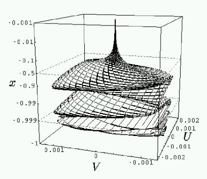
Figure 23: Phase-portrait of the regular continuation of the Choptuik spacetime from the CH at $x_{f}=-1$ to the regular center at $x_{r}=0$. Again, from $x=-1$ to $x=-0.999$ we have distorted the axis to show the infinite number of oscillations that pile up there. From $x=-0.999$ to $x=-0.5$ we use a logarithmic axis and from this middle point to $x=-0.001$ we use a different logarithmic axis.

Imposing CSS means that the system is independent of $\tau$ and hence the phase-portrait in $(U,V,x)$ reduces to a line that can be easily projected on the $(U,V)$ plane. Then the whole evolution of the system can be described by this curve in the $(U,V)$ plane, which is now completely gauge-invariant. This is essentially what Brady has done Brady .

In order to understand the singular continuations of the critical spacetime, we first look at phase portraits of the Roberts spacetime. Fig. 24 shows the phase-lines of the Roberts solution for several values of $p$ in both branches (see also Appendix C). We see that the shape of the curves become constant for very small values of $p$, but just translated along the $\log x$-axis. On the other hand Fig. 25 gives the phase-portrait two of our singular evolutions, for small and large initial $\hat{U}_{\epsilon}$, respectively. In both cases as $U+V\to 0$ squeezes the phase cylinder into the diagonal, following a Roberts solution in the former case, and not doing so in the latter. This figure demonstrates why it is not possible to obtain $a^{2}=2$ in the continuations of the Choptuik solution. The Roberts spacetime with $p=1$ does have $a^{2}=2$ on the singularity, $p=0$ (Minkowski) has $a^{2}=1$, and all other $p$ have $a^{2}\to 0$. The $p=1$ Roberts solution has the phase line $U=V=\pm 1/\sqrt{2}$ line. To reach $a^{2}=2$ approach a solution must approach this line from the very beginning, because it is unstable. This requires $V$ of order $1/\sqrt{2}$ at least and on the Cauchy horizon we only have $V$ of order $10^{-3}$.

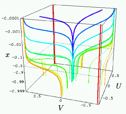
Figure 24: Phase-lines of the Roberts spacetime. The colors encode different values of $p$, for both branches: 1 (red), 0.99 (orange), 0.9 (yellow), 0.5 (light green), 0.1 (dark green), 0.01 (light blue), 0.001 (dark blue) and 0.0001 (purple). The future (past) branch of the singularity is denoted with thick (thin) lines starting with $V=0$ ($U=0$). Note that the vertical lines $U=V=\pm 1/\sqrt{2}$ corresponding to $p=1$ are unstable. Note also that the smaller $p$ is, the longer the curves stay close to the unstable flat line $U=V=0$.

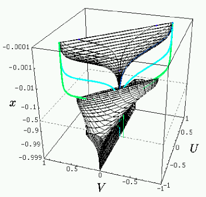
Figure 25: Phase-portrait of two singular continuation of the Choptuik spacetime (upper: initial $\hat{U}_{\epsilon}$ of order $10^{-3}$; lower: initial $\hat{U}_{\epsilon}$ of order $10$), together with a few Roberts solutions for $p=0.1,0.01,0.001$. The $p=0.001$ solution almost coincide with the external envelope of the upper phase-portrait and sets a maximum for the values that are realized in this solution. The lower phase-portrait is shown only for $-0.999<x\leq-0.4$. For $-0.4<x<0$ it is essentially on the diagonal in the $(U,V)$ plane although the amplitude of the oscillations is not the same as in the Roberts solution. Note that for small $x$ this phase portrait has been truncated also in $U$, because $U$ becomes large. For $x\simeq-1$ the phase portrait is essentially on the $U$-axis.

VII Conclusions

In a companion paper spherical_dss we investigate the constraints that the kinematic assumptions of spherical symmetry and discrete self-similarity impose on the causal structure. The key elements of our analysis were the self-similarity horizons – radial null geodesics that are mapped onto themselves by the self-similarity. These come in two types: a “fan” connects a point singularity to a piece of null infinity, while a “splash” connects a piece of null singularity to a point at null infinity. All spherically symmetric and self-similar spacetimes can be enumerated in terms of a sequence of fans and splashes. We found that the singularity is central and consists of a middle segment which is either a point or null line, flanked by two segments which can be timelike, spacelike, or null lines, or which can be absent. There are never two or more disconnected singularities.

In this paper, we have focussed on scalar field matter and in particular Choptuik’s critical solution in gravitational collapse. This solution is found as an intermediate attractor in the evolution of regular asymptotically flat scalar field initial data near the black hole threshold Choptuik . Independently, it can be constructed as the solution of a nonlinear PDE boundary value problem from the assumptions of spherical symmetry, discrete self-similarity, and analyticity at the past center and past lightcone of the singularity critscalar . It can then be uniquely continued up to the future lightcone (Cauchy horizon) of the singularity. Ref. critscalar found that the scalar field oscillates roughly as $\cos(\ln|y|)$ as the Cauchy horizon $y=0$ is approached. It was suggested on theoretical grounds that these oscillations are damped by a factor $|y|^{\epsilon}$ with $\epsilon>0$, but the numerical value of $\epsilon$ was too small to distinguish it from zero numerically.

We have repeated the numerical calculations of Ref. critscalar from scratch and have increased the accuracy by more than four orders of magnitude. We have found the positive value for $\epsilon$ given in Eq. (63). Therefore the scalar field is continuous on the Cauchy horizon, with null data given in Eq. (70). The structure of the fields near the Cauchy horizon is quite complicated, and has been discussed in Subsections III.3 and III.4.

All possible DSS continuations beyond the Cauchy horizon are determined by the (fixed) null data on the Cauchy horizon, and one (arbitrary) periodic function $\hat{U}_{\epsilon}(\hat{\tau})$ that can be thought of as data emerging from the naked singularity. (In the absence of the naked singularity, null data on the Cauchy horizon would alone determine the continuation.) There is a unique DSS continuation that has a regular timelike center except for a naked point singularity. For all other values of the arbitrary function $\hat{U}_{\epsilon}(\hat{\tau})$, the continuation has a timelike central singularity with infinite negative mass. In particular, neither Fig. 3, nor the even more exotic spacetime diagrams found in self-similar perfect fluid solutions fluidcss can arise as continuations of the Choptuik solution (although they can probably arise in other DSS scalar field solutions).

The global structure of the Choptuik solution is of interest partly because of the connection between critical collapse and cosmic censorship. Choptuik’s work has established that (assuming the validity of general relativity at arbitrarily high curvatures) a naked singularity can be formed in the spherical Einstein-scalar field system from generic regular and asymptotically flat initial data by fine-tuning any one parameter to the black hole threshold. Solutions with a naked singularity therefore form a subset of codimension one (the black hole threshold in the space of initial data) in all solutions arising from regular data. The Choptuik spacetime is an attractor on the critical surface and therefore, assuming that it is actually a global attractor on the surface, we can conclude that every naked singularity will have, at least in a neighborhood of the singularity, the structure of the Choptuik spacetime.

We can now summarize this structure as follows: The curvature at the Cauchy horizon of the singularity is finite but not differentiable, with an infinite number of damped oscillations piling up as the Cauchy horizon is approached. The continuation of the spacetime beyond the Cauchy horizon is not unique, but we have shown that if it is DSS then the naked singularity is either a single point or timelike with infinite negative mass. The spacetime near the timelike singularity is locally CSS and velocity-dominated.

The question remains whether this structure is stable against perturbations which break self-similarity and/or spherical symmetry. Because the background is spherically symmetric and periodic in $\tau$, all such perturbations are of the form $e^{\lambda\tau}f(x,\tau)$, where $f(x,\tau)$ is periodic, times a suitable scalar, vector or tensor spherical harmonic. We have shown in the past critscalar ; critscalar2 that all but one of these modes decay, with ${\rm Re}\lambda<0$. (The one growing mode determines the critical exponent for the black hole mass.) The functions $f(x,\tau)$ were calculated explicitly only between the regular center and past lightcone, but as they are by construction analytic at the past lightcone, they can be analytically continued up to the Cauchy horizon, with the same $\lambda$.

What needs to be done is to check that the functions $f(x,\tau)$ remain bounded as $x$ approaches the Cauchy horizon. We expect that this is true. Nolan and Waters NolanWaters have investigated a massless minimally coupled, non-spherically symmetric scalar field propagating on a class of spherically symmetric CSS spacetimes, and find that its gradient remains finite at the Cauchy horizon. The structure of the full perturbation equations is similar.

As the functions $f(x,\tau)$ cannot be analytic at the Cauchy horizon (because the background is not), the spectrum of $\lambda$ need not be the same in the continuation beyond the Cauchy horizon, and is likely to depend on the choice of continuation.

We have finally given, for the first time, a number of global images of the Choptuik spacetime, trying to minimize the gauge content of the pictures.

Appendix A Review of coordinate systems for given $F$

In this Appendix we review a variety of coordinate systems defined by giving $F$ as a function of $\tau$ and $x$. This class covers the coordinate systems used in Refs. OriPiran ; critscalar ; Brady ; Garfinkle2+1 ; GoliathNilssonUggla , but does not include the Lagrangian fluid coordinates used in CarrColey . We classify the gauges within this class in three stages. 1) We fix $F(\tau,x)$. 2) We impose an algebraic relation between $A$, $B$ and $C$. 3) We parameterize $A$, $B$ and $C$ in terms of two functions, say $a$ and $f$. (It will turn out to be useful to always use the scalar $a$ defined above as one of the two parameters.)

In a DSS spacetime, the unknowns are periodic in $\tau$. We therefore solve the Einstein equations by “evolving” in $x$, with periodic boundary conditions in $\tau$. When we use the Einstein equations to eliminate the metric derivative $P$, $U$ and $V$ obey a pair of transport equation of the form

$$U_{,x}=(\dots)\,U_{,\tau}+(\dots),\quad V_{,x}=(\dots)\,V_{,\tau}+(\dots),$$ (94)

where the dots stand for a known function of $U$, $V$, $a$ and $f$ but not their derivatives. By a suitable parameterization of $A$, $B$ and $C$ in terms of $a$ and $f$, the Einstein equations can always be brought into the form of two ODEs in $x$, which for our purposes are evolution equations, and one ODE in $\tau$, which for our purposes is a constraint:

$$f_{,x}=(\dots),\quad a_{,x}=(\dots),\quad a_{,\tau}=(\dots).$$ (95)

This last equation can be made linear in $a^{-2}$ (that is, in $\mu$) by a suitable choice of $f$, at least in all three coordinate systems we use. This inhomogeneous linear equation can then be solved uniquely for $a$ in terms of $U$, $V$ and $f$, using the fact that $U$, $V$ and $f$ are periodic in $\tau$ and that we require $a$ to be periodic, too. In a CSS solution, where nothing depends on $\tau$, the $a_{,\tau}$ constraint becomes an algebraic equation linking $U$, $V$, $a$ and $f$.

A.1 Past patches with $F=x$

The regular center is both timelike and an $x$ line, but $\tau$ is finite there. This requires $F=0$ at the center, and $F>0$ elsewhere. The simplest choice is $F=x$. On a past patch, it is possible to choose the $\tau$ lines to be timelike, null or spacelike, or to change signature. We consider only the first two possibilities

Bondi past patch

If we choose the $\tau$-lines to be null everywhere, this means $C=0$. We then have $B<0$ between the past center and the past light cone, and $B>0$ beyond the past lightcone, so that $A$ and $B$ both change sign at the past lightcone. $F=x$ and $C=0$ has been used by Brady Brady to investigate CSS solutions with scalar field matter. He used the Bondi metric coefficients that are traditionally called $g$ and $\bar{g}$ as parameters. In a DSS solution this gives a constraint for a combination of $g$ and $\bar{g}$, as well as evolution equations for $g$ and $\bar{g}$. The best parameterization we have found uses the mass function $a$ and the Bondi metric coefficient $f=g/a^{2}$:

$$A = -g(\bar{g}\mp 2x)=-a^{2}f(f\mp 2x),$$ (96)

$$B = \mp g=\mp a^{2}f,$$ (97)

$$C = 0,$$ (98)

$$F = x,$$ (99)

where the upper sign applies when $\tau$ is an outgoing null coordinate, and the lower sign applies when $\tau$ is an ingoing null coordinate, assuming that $f>0$. This gives an ODE evolution equation and a linear ODE constraint for $a^{-2}$, and an ODE evolution equation for $f$.

Schwarzschild past patch

If the $\tau$-lines are spacelike everywhere, this implies $C>1$. A natural algebraic condition to impose is to make the $\tau$ lines orthogonal to the $r$ lines. This means $B(\tau,x)=-xC(\tau,x)$. $\tau$ is then $-\ln(-t)$ where $t$ is the Schwarzschild time coordinate. A possible parameterization is in terms of the metric coefficients often called $a$ and $\alpha$ in Schwarzschild coordinates. ($a$ is the scalar we have defined above). The best parameterization we have found is by $a$ and $f=\alpha/a$, and is given in (13) above. It gives ODE evolution equations for $a$ and $f$, and a linear ODE constraint equation for $a^{-2}$. The transport equations for $U$ and $V$ are linear in $U$ and $V$ because $P$ reduces to a function of $a$, $\tau$ and $x$. The lightcones are at $f\pm x=0$ (although of course only one lightcone can be covered at one time by a past patch).

A.2 Outer patches with $F=1$

On an outer patch that stretches from the past to the future lightcone the $\tau$ lines must be timelike at least somewhere, and it is possible to make them timelike everywhere. The simplest choice for $F$ compatible with all these possibilities is $F$=1.

Schwarzschild outer patch

Assuming that the $\tau$ lines are timelike everywhere means $C<0$. We have $B<0$ on the past lightcone and $B>0$ on the future lightcone, so that $B$ has to change sign somewhere between. This “$B$-surface” is where the $\tau$ and $x$ lines are orthogonal. In critscalar one of us used a coordinate system in the outer patch that was based on Schwarzschild coordinates. As in the past patch based on Schwarzschild coordinates, this meant $B=-xC$. However, when we impose $B=-xC$ together with $F=1$, we face an unexpected coordinate singularity at $x=0$. In particular, if we again use $a$ and $f=\alpha/a$ to parameterize the metric, we obtain an ODE constraint and an ODE evolution equation for $a$ as before on the past patch, but for $f$ we obtain an equation of the form

$$f_{,x}={(\dots)f_{,\tau}+(\dots)\over x}$$ (100)

In order to make the coordinates regular at $x=0$, we need to impose the vanishing of the numerator of this equation there, and that is effectively what was done in critscalar . But this introduces an additional boundary condition just to keep the coordinate system regular on a surface where the solution itself is perfectly regular, and that is why we do not use these coordinates here.

Best buy outer patch

A better algebraic condition to combine with $F=1$ is $C=-1$. A workable parameterization is in terms of the mass function $a$ and $B$ itself. This gives ODE evolution equations for $a$ and $B$, and a (nonlinear) ODE constraint for $a$. The lightcones are at $a\pm B=0$. If we replace $B$ by $b=B/a$, we have the parameterization given above in (21), and the ODE constraint for $a$ becomes linear in $a^{-2}$, while the wave equation becomes linear in $U$ and $V$.

$A=-C$: unworkable

It is compatible with $F=1$ to assume that the $\tau$ lines “bend round” to become spacelike at large and small $x$. means This that $C$ changes sign. A natural choice is that $A$ and $C$ change sign together, and we can impose this by setting $A=-C$. We have not found a way of parameterizing this choice in a way that brings the Einstein equations into the standard form (95). Parameterizing with $B$ and $\mu$ gives two roots for $A$. Using $A$ and $\mu$ gives two roots for $B$.

$x$ and $\tau$ orthogonal: unworkable

We can also force the “bending round” by making $\tau$ and $x$ lines orthogonal everywhere, or $B=0$. This implies that, while they are independent, $A$ and $C$ change sign together. Parameterizing by $A$ and $C$ we obtain an evolution equation and a constraint for $A$ and a constraint for $C$. But the constraint for $C$ is homogeneous, $C_{,\tau}=N(A,U,V)C$, so that $C$ cannot be periodic. Therefore this coordinate system is not compatible with CSS or DSS.

Forcing the lightcones: unworkable

Instead of finding a working outer patch and then forcing the two lightcones to fall on the lines $x=x_{p}$ and $x=x_{f}$ by imposing $A(\tau,x_{p})=A(\tau,x_{f})=0$, we can make $A$ a given function of $x$. The simplest such choice is $A=1-x^{2}$, which vanishes at $x=\pm 1$. (The two lightcones will be distinguished by the sign of $B$). A parameterization that brings the Einstein equations into standard form is

$$A=1-x^{2},\quad B=bc,\quad C=-c^{2},\quad F=1.$$ (101)

This gives an evolution equation and a constraint for $b$ and a linear constraint for $c$. However, the right-hand sides of all three equations are of the form $N/b$. Furthermore, at $b=0$ the numerator of $b_{,\tau}$ depends on the matter through $U^{2}+V^{2}$, while the numerator of $b_{,x}$ depends on the matter through $U^{2}-V^{2}$. (The numerator of $c_{,\tau}$ is proportional to that of $b_{,\tau}$.) That means that we would have to impose two independent regularity conditions at $b=0$. Together these would fix $U$ and $V$ completely. Therefore this coordinate system is not sufficiently generic near the line $B=0$.

Appendix B Singular expansion around the Cauchy horizon

From (46,47) we see that

$$D=yD_{1}(\tau)+y^{2}D_{2}(\tau)+O\left(|y|^{2+\epsilon}\right),$$ (102)

The regular coefficients to $O(y)$ are as follows: $U_{1}(\tau)$ is the unique periodic solution of

$$U_{1}^{\prime}+(1-a_{0}^{2}-D_{1})U_{1}+V_{1}-2a_{0}a_{1}U_{0}=0,$$ (103)

and

$$V_{1} = -{\xi\over 2a_{0}}\left[(1-a_{0}^{2})V_{0}+U_{0}+V_{0}^{\prime}\right],$$ (104)

$$a_{1} = -{\xi\over 2}(U_{0}^{2}-V_{0}^{2}),$$ (105)

$$b_{1} = -{\xi^{\prime}\over a_{0}}-{\xi\over 2a_{0}}\left(-3+a_{0}^{2}+2V_{0}^{2}\right),$$ (106)

$$b_{2} = -{a_{1}\over 2a_{0}}b_{1}$$ (107)

$$-{\xi\over 4a_{0}}\left(2a_{0}a_{1}-b_{1}U_{0}^{2}+b_{1}V_{0}^{2}+4V_{0}V_{1}\right),$$

$$D_{1} = -{a_{0}b_{1}\over\xi}.$$ (108)

The regular coefficients to higher orders continue in this style, with $U_{n}(\tau)$ the solution of a linear inhomogeneous ODE, while $V_{n}$, $a_{n}$ and $b_{n}$ are given algebraically.

The nonvanishing singular coefficients up to $O(y^{1+3\epsilon})$ are

$$a_{1+\epsilon}(\tau,x) = \check{a}_{1+\epsilon}(\tau)\hat{a}_{1+\epsilon}(\hat{\tau}),$$ (109)

$$a_{1+2\epsilon}(\tau,x) = \check{a}_{1+2\epsilon}(\tau)\hat{a}_{1+2\epsilon}(\hat{\tau}),$$ (110)

$$V_{1+\epsilon}(\tau,x) = \check{V}_{1+\epsilon}(\tau)\hat{V}_{1+\epsilon}(\hat{\tau}),$$ (111)

$$U_{1+\epsilon}(\tau,x) = \sum_{i=1}^{3}\check{U}_{1+\epsilon}^{(i)}(\tau)\hat{U}_{1+\epsilon}^{(i)}(\hat{\tau}),$$ (112)

$$U_{1+2\epsilon}(\tau,x) = \sum_{i=1}^{7}\check{U}_{1+2\epsilon}^{(i)}(\tau)\hat{U}_{1+2\epsilon}^{(i)}(\hat{\tau}),$$ (113)

$$U_{1+3\epsilon}(\tau,x) = \sum_{i=1}^{6}\check{U}_{1+3\epsilon}^{(i)}(\tau)\hat{U}_{1+3\epsilon}^{(i)}(\hat{\tau}).$$ (114)

We only give two examples of how these coefficients are derived. Substituting the ansatz into the $a_{,x}$ equation and isolating the terms of $O(y^{\epsilon})$ in the result, we obtain

$$(1+\epsilon)\check{a}_{1+\epsilon}(\tau)\hat{a}_{1+\epsilon}(\hat{\tau})+K\check{a}_{1+\epsilon}(\tau)\hat{a}_{1+\epsilon}^{\prime}(\hat{\tau})=$$

$$-\xi(\tau)U_{0}(\tau)\check{U}_{\epsilon}(\tau)\hat{U}_{\epsilon}(\hat{\tau}).$$ (115)

We solve this for all $\tau$ and $\hat{\tau}$ by setting

$$\check{a}_{1+\epsilon}(\tau)={\xi(\tau)U_{0}(\tau)\check{U}_{\epsilon}(\tau)\over K}$$ (116)

and by making $\hat{a}_{1+\epsilon}(\hat{\tau})$ the unique solution of the ODE

$$\hat{a}_{1+\epsilon}^{\prime}+{1+\epsilon\over K}\hat{a}_{1+\epsilon}+\hat{U}_{\epsilon}=0.$$ (117)

If we substitute the ansatz into the $U_{,x}$ equation (27) and isolate the terms of $O(y^{1+\epsilon})$, we find

$$D_{1}\left((1+\epsilon)\sum_{i}\check{U}_{1+\epsilon}^{(i)}\hat{U}_{1+\epsilon}^{(i)}+K\sum_{i}U_{1+\epsilon}\hat{U}_{1+\epsilon}^{\prime(i)}\right)+D_{2}\left((1+\epsilon)\check{U}_{\epsilon}\hat{U}_{\epsilon}+KU_{\epsilon}\hat{U}_{\epsilon}^{\prime}\right)$$

$$=(1-a_{0}^{2})\sum_{i}U_{1+\epsilon}^{(i)}\hat{U}_{1+\epsilon}^{(i)}-2a_{0}a_{1}\check{U}_{\epsilon}\hat{U}_{\epsilon}-2a_{0}\check{a}_{1+\epsilon}\hat{a}_{1+\epsilon}U_{0}+\check{V}_{1+\epsilon}\hat{V}_{1+\epsilon}+\sum_{i}\check{U}_{1+\epsilon}^{\prime(i)}\hat{U}_{1+\epsilon}^{(i)}+(1+H^{\prime})\sum_{i}\check{U}_{1+\epsilon}^{(i)}\hat{U}_{1+\epsilon}^{\prime(i)}$$ (118)

Because $KD_{1}=1+H^{\prime}$, the derivatives $\hat{U}_{1+\epsilon}^{\prime(i)}$ cancel out. Taking also into account that $\hat{V}_{1+\epsilon}=\hat{a}_{1+\epsilon}$ (this is an accident at this particular order), the equation can be rewritten as

$$\sum_{i}\left[\check{U}_{1+\epsilon}^{\prime(i)}+\left(1-a_{0}^{2}-(1+\epsilon)D_{1}\right)\check{U}_{1+\epsilon}^{(i)}\right]\hat{U}_{1+\epsilon}^{(i)}$$

$$+\left[-\epsilon D_{2}-2a_{0}a_{2})\check{U}_{\epsilon}\right]\hat{U}_{\epsilon}+\left[-KD_{2}\check{U}_{\epsilon}\right]\hat{U}_{\epsilon}^{\prime}+\left[\check{V}_{1+\epsilon}-2a_{0}\check{a}_{1+\epsilon}U_{0}\right]\hat{a}_{1+\epsilon}=0.$$ (119)

The terms in square brackets all depend on $\tau$ and each multiplies a different known function of $\hat{\tau}$. To solve this for all $\tau$ and $\hat{\tau}$, we assign one term $\hat{U}_{1+\epsilon}^{(i)}$ to each function of $\hat{\tau}$:

$$\hat{U}_{1+\epsilon}^{(1)}=\hat{U}_{\epsilon},\quad\hat{U}_{1+\epsilon}^{(2)}=\hat{U}_{\epsilon}^{\prime},\quad\hat{U}_{1+\epsilon}^{(3)}=\hat{a}_{1+\epsilon}.$$ (120)

The corresponding coefficients $\check{U}_{1+\epsilon}^{(i)}$ are the unique solutions of the ODEs

$$\check{U}_{1+\epsilon}^{\prime(i)}+\left(1-a_{0}^{2}-(1+\epsilon)D_{1}\right)\check{U}_{1+\epsilon}^{(i)}+S^{(i)}=0,$$ (121)

where the source terms $S^{(i)}$ can be read off directly from (B). The calculation of the other terms proceeds in a similar manner at all orders. Note that the functions of type $\check{f}$, where $f$ stands for $V$, $a$ and $b$, are given algebraically and $\hat{f}$ obeys an ODE. For $U$ it is the other way around.

The limit $V_{0}=0\Leftrightarrow\epsilon=0$ of our expansion exists. The regular $O(y^{n})$ terms in the series vanish identically, and so do some of the $O(|y|^{n+k\epsilon}$ terms but not all of them. $a_{1}$ and $a_{1+\epsilon}$ for example vanish because they are proportional to $U_{0}$, but $a_{1+2\epsilon}$ is proportional to $U_{\epsilon}^{2}$, and so encodes the curvature to $O(y)$.

In the limit $\epsilon=0$ the curvature components proportional to $U^{2}$ are no longer continuous at the CH because they are now periodic in $\hat{\tau}=\tau-\ln|y|$, but for the same reason they remain bounded. The components proportional to $UV$ and $V^{2}$ are still continuous even then because $V$ is $O(y)$. $a$ is also still continuous, with $a=1$ on the Cauchy horizon.

Appendix C The Roberts solution

In the notation of Oshiro , the Roberts solution Roberts is given by

$$ds^{2} = -du\,dv+r^{2}(u,v)\,d\Omega^{2},$$ (122)

$$r^{2}(u,v) = \frac{1}{4}\left[(1-p^{2})v^{2}-2vu+u^{2}\right],$$ (123)

$$\phi(u,v) = \frac{1}{\sqrt{16\pi G}}\log\frac{(1-p)v-u}{(1+p)v-u},$$ (124)

with $p$ a constant parameter. $p=0$ is Minkowski spacetime with zero scalar field, and without loss of generality $p\geq 0$. Only the regions $r^{2}>0$ are physical and without loss of generality, we consider the right side ($v-u>0$) of the spacetime.

For $p\neq 0$, the lines $u=(1\pm p)v$ are central curvature singularities: the mass function $\mu=-p^{2}uv/(4r^{2})$ diverges on them. The line $u=(1+p)v$, $v<0$ is timelike and has (infinite) negative mass, and for $v<0$ forms the past branch of the Roberts singularity. The line $u=(1-p)v$ is timelike with negative mass for $p<1$, null with zero mass for $p=1$, and spacelike with positive mass $p>1$. For $v>0$ it forms the future segment of the singularity.

Some of our solutions become asymptotically CSS and have $\kappa\simeq 0$, therefore approaching the Roberts spacetime. We know that the solutions develop a timelike, negative mass singularity, which must correspond to one of the two branches of the Roberts singularity. In this Appendix we study the issue of which of the two branches is actually approached in our numerical evolutions and for what values of $p$.

Our scalars $U$ and $V$ are

$$U=-\frac{p}{\sqrt{2}}\,\frac{v}{v-u},\qquad V=\frac{p}{\sqrt{2}}\,\frac{u}{v-u-p^{2}v},$$ (125)

where both denominators are positive in the region of interest. It is clear that $p$ is covariantly defined by $U$ and $V$ on the light cones $u=0$ or $v=0$, respectively. However, at the singularities $u=(1\pm p)v$ the scalars take values $U=-V=\pm 1/\sqrt{2}$ for any $0\neq p\neq 1$ in the Roberts solution. If we use an expansion using a generic self-similar coordinate $y$ such that $u/v=F(y)$ with the singularity at $y=0$ [that is, $F(0)=1\pm p$]:

$$\sqrt{2}\,U(y) = \pm 1-\frac{y}{p}F^{\prime}(0)+O(y^{2}),$$ (126)

$$\sqrt{2}\,V(y) = \mp 1+\frac{y}{p}\frac{1\mp p}{1\pm p}F^{\prime}(0)+O(y^{2}).$$ (127)

Therefore $p$ is covariantly given by the ratio of the rates at which $U$ and $V$ approach their values at the singularity:

$$\lim_{x\to 0}{dU\over dV}=-\frac{1\pm p}{1\mp p}.$$ (128)

This determines both $p$ and which branch of the singularity we approach locally: The upper sign applies for $|dU/dV|>1$ (past branch, turned upside down) and the lower sign for $|dU/dV|<1$ (future branch of the singularity).

We can relate the coordinates $(u,v)$ of (122-124) to our coordinate $x$ through

$$\left(1-\frac{u}{v}\right)^{2}=p^{2}+(1-p^{2})x^{2}.$$ (129)

This expression applies only for negative $x$ and so only covers the future branch of the singularity. We obtain the expressions for the past branch exchanging the role of the functions $U$ and $V$. That explains why exchanging $U$ and $V$ in Eq. (128) amounts to a change of branch. It also shows that we have to change branch four times per $\Delta$-period as we move through the four quadrants determined by the lines $U+V=0$ and $U-V=0$.

References

- (1) M. W. Choptuik, Phys. Rev. Lett. 70, 9 (1993).
- (2) A. M. Abrahams and C. R. Evans, Phys. Rev. Lett. 70, 2980 (1993).
- (3) C. Gundlach, Living Reviews in Relativity 2, 4 (1999), published electronically at http://www.livingreviews.org. For an updated version see C. Gundlach, Critical phenomena in gravitational collapse, to be published in Phys. Rep., preprint gr-qc/0210101.
- (4) C. Gundlach and J. M. Martín-García, Kinematics of discretely self-similar spherically symmetric spacetimes, in preparation.
- (5) C. Gundlach, Phys. Rev. D 55, 695 (1997).
- (6) B. C. Nolan, Class. Quant. Grav. 18, 1651 (2001).
- (7) A. Ori and T. Piran, Phys. Rev. Lett. 59, 2137 (1987).
- (8) B. J. Carr and C. Gundlach, Phys. Rev. D 67, 024035 (2003).
- (9) A. Iserles, Numerical Analysis of Differential Equations, Cambridge University Press, 1996.
- (10) L. Andersson and A. D. Rendall, Commun. Math. Phys. 218 479 (2001).
- (11) M. D. Roberts, Gen. Rel. Grav. 21, 907-939 (1989).
- (12) P. Brady, Phys. Rev. D 51, 4168 (1995).
- (13) J. M. Martín-García and C. Gundlach, Phys. Rev. D 59, 064031 (1999).
- (14) B. C. Nolan and T. J. Waters, Phys. Rev. D 66, 104012 (2002).
- (15) D. Garfinkle, Phys. Rev. D 63, 044007 (2001).
- (16) B. J. Carr, A. A. Coley, M. Goliath, U. S. Nilsson, and C. Uggla, Class. Quant. Grav. 18, 303 (2001).
- (17) B. J. Carr and A. A. Coley, Phys. Rev. D 62, 044023 (2000).
- (18) Y. Oshiro, K. Nakamura, and A. Tomimatsu, Prog. Theor. Phys. 91, 1265 (1994).