Inhomogeneous cosmologies with tachyonic dust as dark matter

Abstract

A cosmology is considered driven by a stress-energy tensor consisting of a perfect fluid, an inhomogeneous pressure term (which we call a “tachyonic dust” for reasons which will become apparent) and a cosmological constant. The inflationary, radiation dominated and matter dominated eras are investigated in detail. In all three eras, the tachyonic pressure decreases with increasing radius of the universe and is thus minimal in the matter dominated era. The gravitational effects of the dust, however, may still strongly affect the universe at present time. In case the tachyonic pressure is positive, it enhances the overall matter density and is a candidate for dark matter. In the case where the tachyonic pressure is negative, the recent acceleration of the universe can be understood without the need for a cosmological constant. The ordinary matter, however, has positive energy density at all times. In a later section, the extension to a variable cosmological term is investigated and a specific model is put forward such that recent acceleration and future re-collapse is possible.

PACS numbers: 95.35.+d, 98.80.-k
Key words: inhomogeneous cosmology, tachyon

1 Introduction

There are compelling reasons to study a cosmology which is not homogeneous. Inhomogeneous models were studied early on by Lemaître [1] and Tolman [2] and by many authors since. Misner [3], for example, postulated a chaotic cosmology in which the universe began in a highly irregular state but which becomes regular at late times. The models presented here possess exactly this property, which will be realized in a later section. That is, in the matter phase, the deviation from FLRW spatial geometry is minimal and we show this by calculating the Gaussian curvature of two spheres in all phases. The curvature of a two sphere is the same for all values of $r$ in the matter domain yielding a three-dimensional space which is isometric to a sphere. Our present location may therefore be anywhere in this universe and there is no conflict with observational cosmology. The book by Krasiński also contains many inhomogeneous models which do not require us to be located at the center of symmetry [4]. Some more recent studies dealing with inhomogeneous cosmologies include [5], [6], [7], [8], [9], [10] and [11].

Inhomogeneous cosmological models are not at odds with astrophysical data. It is well known that inhomogeneities in the early universe will generate anisotropies in the cosmic microwave background radiation (CMB). Such effects have been studied by many groups ([12], [13], [14], [15]) using density amplitudes and sizes of inhomogeneities corresponding to those of observed current objects (galactic clusters, the Great Attractor and voids). These studies, utilizing a range of reasonable parameters, have found that temperature fluctuations in the CMB, $\Delta T/\langle T\rangle$, ($\langle T\rangle$ being the mean temperature and $\Delta T$ the deviation from the mean) amount to no more than about $10^{-7}-10^{-5}$, which is compatible with observation. Also, arguments to reconcile inhomogeneous solutions with cosmological observations may be found in [10]. The inhomogeneity referred to in this paper is a “radial” inhomogeneity compatible with spherical symmetry and therefore its effect on the CMB is potentially more difficult to detect than the (small) angular deviations.

In general, at very high energies, our knowledge of the state of the universe is highly limited and special assumptions about the matter content and symmetry should be relaxed. It therefore seems reasonable to investigate solutions which, at least at early times, are less symmetric than the FLRW scenarios. A thorough exposition on various inhomogeneous cosmological models may be found in the book by Krasiński [4].

In section 2 we consider a cosmology consisting of two fluids, a perfect fluid (motivated by the successful standard cosmology) and “tachyonic” dust. We use the term tachyonic due to the association of this source with space-like vectors in the stress-energy tensor. This terminology is also popular in string-theory motivated cosmologies commenced by the pioneering works of Mazumdar, Panda, Pérez-Lornezana [16] and Sen [17] and studied by many others (see, for example, [18], [19], [20], [21], [22], [23], [24], [25], [26], [27], [28] [29] and references therein). It should be pointed out that in neither the case presented here nor the string theory motivated case is the source acausal as will be pointed out below .

The tachyonic dust is chosen as a dark matter candidate for several reasons. First, it provides one of the simplest extensions to the standard perfect fluid cosmology and it is hoped that this model will provide insight into more complex scenarios. Second, as will be seen below, the tachyonic dust is a source of pressure or tension without energy density and cosmological observations strongly imply that there exists a large pressure or tension component in our universe. This pressure also affects the overall effective mass of the universe. Multi-fluid models in the context of charged black holes in cosmology have been studied in [30]

In section 3 we consider an extension of the model to the case of variable cosmological term. We discuss in detail how making this term dynamical affects the fate of the universe.

Finally, this paper utilizes a number of techniques for analyzing global properties of the manifold and it is hoped that this will provide a useful reference for the mathematical analysis of cosmological models.

2 Tachyonic dust and perfect fluid universe

We consider here a model of the universe which contains both a perfect fluid and tachyonic dust. This source possesses the desirable properties mentioned in the introduction. Namely, the dust contribution is a source of pressure as is required for the recent accelerating phase of the universe. A tachyonic dust is the simplest model which contributes to pressure and it will be shown that this pressure also makes a contribution to the mass of the universe. This field is therefore also a potentially interesting candidate for dark matter.

Aside from spherical symmetry, the sole assumption is that the eigenvalues of stress-energy tensor be real. We may therefore write

$$T^{\mu}_{\;\nu}=\left[\mu(t,r)+p(t,r)\right]u^{\mu}u_{\nu}+p(t,r)\delta^{\mu}_{\;\nu}+\alpha(t,r)w^{\mu}w_{\nu},$$ (1)

with

$$u^{\beta}u_{\beta}=-1,\;\;\;\;\;w^{\beta}w_{\beta}=+1,\;\;\;\;\;u^{\beta}w_{\beta}=0.$$

Here $\mu(t,r)$, $p(t,r)$ and $\alpha(t,r)$ are the fluid energy density, fluid pressure, and tachyonic pressure (or tension) respectively. By comparison of the $\alpha(t,r)$ term in (1) to the stress-energy tensor of regular dust, it can be seen why we choose the term “tachyonic dust” to describe this source. Notice that a dust associated with a space-like vector possesses the desirable property in that it yields solely a pressure. It will be shown that this tension may produce the observed acceleration of the universe at late times [31], [32]. The source is not acausal as the algebraic structure of (1) is exactly similar to that of an anisotropic fluid which is a causal source under minor restrictions and is often used in general relativity (see [33], [34], [35] and references therein).

The time coordinate, $t$, may be chosen to be coincident with the proper time along a fluid streamline (the comoving condition). This gauge, along with spherical symmetry, allows a special class of metrics to be written as

$$d\sigma^{2}:= \left[\frac{dr^{2}}{1-\epsilon r^{2}+eg(r)}+r^{2}\,d\theta^{2}+r^{2}\sin^{2}\theta\,d\phi^{2}\right],$$ (2a)

$$ds^{2}= -dt^{2}+a^{2}(t)\,d\sigma^{2}.$$ (2b)

This form is particularly convenient as one may readily analyze differences between models presented here and the standard FLRW models (the $e\rightarrow 0$ limit). Therefore, $e$ may be interpreted as the tachyon coupling constant. It is easy to show that (2a-2b) falls in the Tolman-Bondi class of metrics, used extensively in studies of inhomogeneous cosmologies.

Using (1) and (2b) in the Einstein equations with cosmological constant yields:

$$8\pi\mu(t,r)+\Lambda= 3\left[\frac{\dot{a}(t)}{a(t)}\right]^{2}+\frac{3\epsilon}{a^{2}(t)}-\frac{e}{r^{2}a^{2}(t)}\left[rg(r)\right]^{\prime},$$ (3a)

$$8\pi p(t,r)-\Lambda= -2\frac{\ddot{a}(t)}{a(t)}-\left[\frac{\dot{a}(t)}{a(t)}\right]^{2}-\frac{\epsilon}{a^{2}(t)}+\frac{eg^{\prime}(r)}{2ra^{2}(t)},$$ (3b)

$$8\pi\alpha(t,r)= -\frac{er}{2a^{2}(t)}\left[\frac{g(r)}{r^{2}}\right]^{\prime},$$ (3c)

where dots represent partial derivatives with respect to $t$ and primes with respect to $r$.

Enforcing conservation on (1) yields two non-trivial equations:

$$\mu(t,r)_{,t}+\frac{\dot{a}(t)}{a(t)}\left\{3\left[\mu(t,r)+p(t,r)\right]+\alpha(t,r)\right\} =0,$$ (4a)

$$\left[p(t,r)+\alpha(t,r)\right]_{,r}+\frac{2\alpha(t,r)}{r} =0.$$ (4b)

Throughout this paper, restrictions $a(t)>0$, $\dot{a}(t)\neq 0$ and $r>0$ are assumed in solving the differential equations. In case the tachyon parameter $e=0$, one gets back the standard FLRW cosmology.

The orthonormal Riemann components will be useful:

$$R_{\hat{t}\hat{r}\hat{t}\hat{r}}= -\frac{\dot{a}(t)}{a(t)}=R_{\hat{t}\hat{\theta}\hat{t}\hat{\theta}},$$ (5a)

$$R_{\hat{r}\hat{\theta}\hat{r}\hat{\theta}}\equiv R_{\hat{r}\hat{\phi}\hat{r}\hat{\phi}}= \frac{1}{a^{2}(t)r}\left[r\dot{a}^{2}(t)+\epsilon r-\frac{eg^{\prime}(r)}{2}\right],$$ (5b)

$$R_{\hat{\theta}\hat{\phi}\hat{\theta}\hat{\phi}}= \left[\frac{\dot{a}(t)}{a(t)}\right]^{2}+\frac{2\epsilon r-eg^{\prime}(r)}{ra(t)^{2}},$$ (5c)

as well as those related by symmetry (hatted indices denote the orthonormal frame). The solutions, being local and valid in some domain, need not possess the neighbourhood near $r=0$. The singularity at $r=0$ will be addressed in a later section.

In cosmology, two measurable parameters considered are the Hubble parameter $H(t)$ and the deceleration parameter, $q(t)$. These are:

$$H(t):= \frac{\dot{a}(t)}{a(t)}=-R_{\hat{t}\hat{r}\hat{t}\hat{r}},$$ (6a)

$$q(t):= -\frac{a(t)\ddot{a}(t)}{\dot{a}^{2}(t)}.$$ (6b)

The field equations, (3a), (3b) and (3c) yield

$$\left[H(t)\right]^{2}= \frac{8\pi}{3}\mu(t,r)+\frac{\Lambda}{3}-\frac{\epsilon}{a^{2}(t)}+\frac{e\left[rg(r)\right]^{\prime}}{3r^{2}a^{2}(t)},$$ (7a)

$$6q(t)\left[H(t)\right]^{2}= 8\pi\left[\mu(t,r)+3p(t,r)\right]-2\Lambda-\frac{er}{2a^{2}(t)}\left[\frac{g(r)}{r^{2}}\right]^{\prime},$$ (7b)

$$\left[H(t)\right]^{2}\left[2q(t)-1\right]= 8\pi p(t,r)-\Lambda+\frac{1}{a^{2}(t)}\left[\epsilon-\frac{eg^{\prime}(r)}{2r}\right].$$ (7c)

To study inhomogeneity, the orthonormal Riemann components of the three-dimensional sub-space (2a) are useful:

$$\tilde{R}_{\hat{r}\hat{\theta}\hat{r}\hat{\theta}}\equiv\tilde{R}_{\hat{r}\hat{\phi}\hat{r}\hat{\phi}}= \epsilon-\frac{eg^{\prime}(r)}{2r},$$ (8a)

$$\tilde{R}_{\hat{\theta}\hat{\phi}\hat{\theta}\hat{\phi}}= \epsilon-\frac{eg(r)}{r^{2}}.$$ (8b)

where the tilde is used to denote quantities calculated using the three dimensional subspace metric of $t=t_{0}$ spatial hyper-surfaces (2a).

Finally, it is useful to define a measure of the inhomogeneity of the spatial universe via an inhomogeneity parameter:

$$I(r):= \frac{\tilde{R}_{\hat{r}\hat{\theta}\hat{r}\hat{\theta}}}{\tilde{R}_{\hat{\theta}\hat{\phi}\hat{\theta}\hat{\phi}}}$$ (9a)

$$= \frac{r\left[2\epsilon r-eg^{\prime}(r)\right]}{2\left[\epsilon r^{2}-eg(r)\right]}.$$ (9b)

A homogeneous space is characterized by $\frac{dI(r)}{dr}\equiv 0$. Specifically, for the FLRW ($e=0$) limit, $I(r)\equiv 1$.

We next investigate the three major eras of cosmological evolution.

2.1 Matter dominated era

In the universe’s recent history, the galaxies which constitute the bulk of the ordinary matter have negligible motion relative to the cosmic expansion. Therefore the pressure of ordinary matter is approximately zero. Reasonable physics also demands that $\mu(t,r)>0$. Setting the pressure equal to zero from the equation (3b) yields (assuming $\dot{a}(t)\neq 0$)

$$\frac{\left[a(t)\dot{a}^{2}(t)\right]^{\cdot}}{\dot{a}(t)}-\Lambda a^{2}(t)=-\left[\epsilon-\frac{e}{2r}g^{\prime}(r)\right]=-C=\mbox{a constant}.$$ (10)

Here, $C$ is the constant of separation. Solving this equation for $g(r)$ one obtains

$$eg(r)=\left(\epsilon-C\right)r^{2}+eb,$$ (11)

with $b$ a constant arising from integration.

The equation for the expansion factor can be analyzed using techniques, many of which are well known in cosmology. We include details here for completion. The equation, after an integration, may be written as:

$$\frac{1}{2}\dot{a}^{2}(t)-\frac{M_{0}}{a(t)}-\frac{\Lambda}{6}a(t)^{2}=-\frac{C}{2}.$$ (12)

Here $M_{0}$ is a constant arising from the integration. In the standard cosmology this equation is often compared to total energy conservation and similar equations have been studied at least as early as Lemaitré and Eddington [37] [38]. The terms on the left hand side correspond to a kinetic energy, gravitational potential energy and vacuum energy respectively. The total energy being constant, $\left(-C/2\right)$. The constant $M_{0}$ may therefore be interpreted as an effective mass of the universe and it is of interest to investigate how the tachyon affects this constant.

The equation (12) may be used in (3a) along with (11) to give the current effective mass of the universe:

$$M_{0}=\mu(t,r)\left[\frac{4}{3}\pi a^{3}(t)\right]+\frac{eb}{6r^{2}}a(t).$$ (13)

The second term in this equation gives the tachyonic contribution to the effective mass of the universe and therefore represents the present mass due to dark matter (which is independent of $\Lambda$ in this section).

The fluid and tachyonic energy density and pressures are given by:

$$8\pi\mu(t,r)= -\Lambda+3\left[\frac{\dot{a}(t)}{a(t)}\right]^{2}+\left(3C-\frac{eb}{r^{2}}\right)\frac{1}{a^{2}(t)},$$ (14a)

$$8\pi p(t,r)\equiv 0,$$ (14b)

$$8\pi\alpha(t,r)= \frac{eb}{r^{2}a^{2}(t)}.$$ (14c)

Note that the tachyon pressure can be very small today (for large $a(t)$) although its effects through (13) can be very large.

Acceleration in the matter phase may be analyzed by studying the equations (7b) and (7c):

$$2q-1= \frac{1}{\dot{a}^{2}(t)}\left[C-\Lambda a^{2}(t)\right],$$ (15a)

$$H^{2}(t)\left(2q-1\right)= \frac{C}{a(t)}-\Lambda,$$ (15b)

$$q= \mu(t,r)\left[\frac{4}{3}\pi\frac{a^{2}(t)}{\dot{a}^{2}(t)}\right]+\frac{eb}{6r^{2}\dot{a}^{2}(t)}-\frac{\Lambda}{3}\frac{a^{2}(t)}{\dot{a}^{2}(t)}.$$ (15c)

Note that for positive $\mu(t,r)$, $q$ may be negative even with $\Lambda=0$. This result indicates that the tachyonic dust may drive the relatively recent acceleration phase indicated by supernova observations [31], [32], [36]. (Recall that positive acceleration corresponds to a negative deceleration parameter.) We will discuss in a later section the values the parameters in (15c) must possess for this scenario. However, the emphasis in this paper will be on Lambda driven acceleration, the tachyon assuming the role of dark matter.

Acceleration can also be studied by differentiating (12) to obtain

$$\ddot{a}(t)=-\frac{M_{0}}{a^{2}(t)}+\frac{\Lambda}{3}a(t).$$ (16)

The above “force” equation nicely demonstrates the fact that positive $M_{0}$ tends to produce an attractive force whereas positive $\Lambda$ produces a negative or repulsive force. The tachyonic effect is inherent in $M_{0}$ via (13).

The fate of the universe is governed by the scale factor, $a(t)$. In general, the equation for $a(t)$ cannot be solved explicitly. Here we use effective potential techniques to study properties of $a(t)$. Figure 1 shows plots of the effective potentials due to the matter fields (grey line indicating the function $-M_{0}/a(t)$) and the cosmological term (dashed line indicating the function $-\frac{\Lambda}{6a^{2}(t)}$) as well as the sum of the two (solid) for various signs of $M_{0}$ and $\Lambda$.

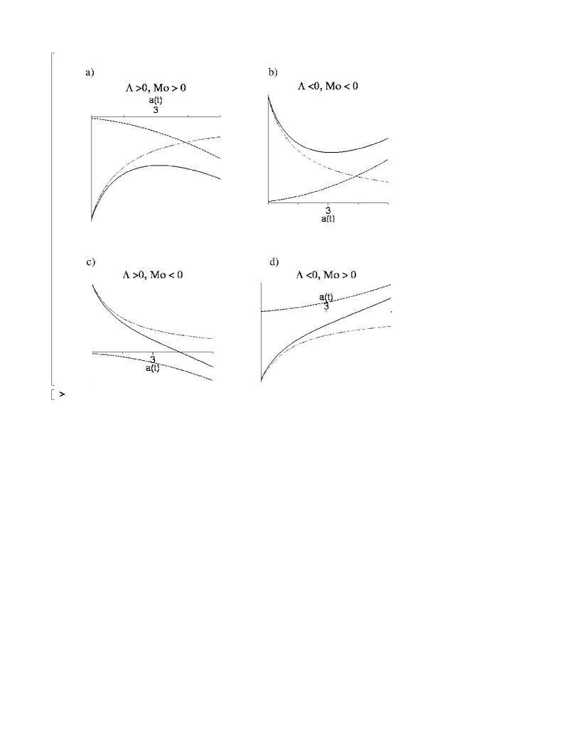
Figure 1: Effective potentials in the matter phase. Dashed lines denote cosmological potential, $-\frac{\Lambda}{6a^{2}(t)}$, grey lines denote matter potential, $-\frac{M_{0}}{a(t)}$, and solid black lines denote net effective potential. Re-collapse is possible for scenarios (a), (b) and (d). Parameters to produce the graphs are $|\Lambda|=0.1$ and $|M_{0}|=1$ although the qualitative picture remains unchanged for other values.

From the figure it can be seen that for $C>0$ situations depicted in figures 1 (a) and (d) allow solutions which re-collapse even for $\Lambda=0$. For $C<0$, the configurations in figures 1 (b) and (d) allow for re-collapse (there are no re-collapse solutions for $C<0$ if $\Lambda=0$). In 2 (c) re-collapse is impossible.

It is of interest to study the geometry of spatial sections generated by this solution. As mentioned in the introduction, the space-like hyper-surfaces are not surfaces of constant curvature. As well, if we consider the global picture, then the parameters discussed can also affect the topology of the universe. Spatial hyper-surfaces at $t=t_{0}$ possess the line element (equation 2a except for a scale factor)

$$d\sigma^{2}=\frac{dr^{2}}{1-Cr^{2}+eb}+r^{2}\,d\theta^{2}+r^{2}\sin^{2}\theta\,d\phi^{2}.$$ (17)

Although (17) bears a close resemblance to the standard FLRW line element, they are not equivalent. The orthonormal Riemann components for (17) yield:

$$\tilde{R}_{\hat{r}\hat{\theta}\hat{r}\hat{\theta}}= C,$$ (18a)

$$\tilde{R}_{\hat{\theta}\hat{\phi}\hat{\theta}\hat{\phi}}= C-\frac{eb}{r^{2}},$$ (18b)

and therefore, for $e\neq 0$, the three dimensional hyper-surfaces are not of constant curvature. For small $e$ deviations are minimal and for $e=0$, the hyper-surface is of constant curvature $C$. The inhomogeneity parameter (9b) is calculated to be

$$I(r)=\frac{{Cr}^{2}}{{Cr}^{2}-eb}.$$ (19)

If we wish to treat the solutions as global, then the spatial topology may be studied. The two dimensional sub-manifold ($\theta=\pi/2$) of the three-metric (17) possesses line element

$$d\sigma_{(2)}^{2}=\frac{dr^{2}}{1-Cr^{2}+eb}+r^{2}\,d\phi^{2}.$$ (20)

Transforming to the arc-length parameter, $l$, along a $r$-coordinate curve, one can obtain

$$d\sigma_{(2)}^{2}=\frac{\left[r^{\prime}(l)\right]^{2}}{A-Cr^{2}(l)}\,dl^{2}+r^{2}(l)\,d\phi^{2}=dl^{2}+r^{2}(l)\,d\phi^{2},$$ (21)

with $A:=1+eb\,$ and $\left[r^{\prime}(l)\right]^{2}=A-Cr^{2}(l)$. Integrating for $r(l)>0$, the following solutions are derived:

$$r(l)=\left\{\begin{array}[]{lll}\sqrt{\frac{A}{2C}}\sin\left[\sqrt{C}(l-l_{0})\right]&\mbox{ for }&C>0\;,\;A>0\\ \sqrt{\frac{A}{2|C|}}\sinh\left[\sqrt{|C|}\left(l-l_{0}\right)\right]&\mbox{ for }&C<0\;,\;A>0\\ \sqrt{\frac{A}{2}}\left(l-l_{0}\right)&\mbox{ for }&C=0\;,\;A>0\;,\end{array}\right.$$ (22)

($l_{0}$ is a constant arising from integration). It is clear from (21) that $l$ is a geodesic coordinate. From the periodicity of the sine function, it may be seen that the two conjugate points on the radial geodesic congruences are given by $\,r(l_{0})=r(l_{0}+\pi/\sqrt{C})=0$. Thus, one concludes that spatially closed universes correspond only to $C>0$.

2.2 Radiation dominated era

Here we study the next major phase in the evolution of the universe. The radiation dominated phase is characterized by the relativistic fluid equation of state $\mu(t,r)=3p(t,r)$. Using this along with (3a) and (3b) yields:

$$\frac{1}{2}\left[a^{2}(t)\right]^{\cdot\cdot}-\frac{2}{3}\Lambda a^{2}(t)=-\epsilon+\frac{5e}{12r^{7/5}}\left[r^{2/5}g(r)\right]^{\prime}=-C,$$ (23)

again $C$ is a separation constant. The equation for $g(r)$ is satisfied by

$$eg(r)=\left(\epsilon-C\right)r^{2}+\frac{eb}{r^{2/5}}.$$ (24)

Solving for the scale factor, $a(t)$, one obtains:

$$a^{2}(t)=\left\{\begin{array}[]{lll}-Ct^{2}+\kappa_{1}t+\kappa_{2}&\mbox{ for }&\Lambda=0\\ \kappa_{1}e^{2\sqrt{\frac{\Lambda}{3}}t}+\kappa_{2}e^{-2\sqrt{\frac{\Lambda}{3}}t}+\frac{3C}{2\Lambda}&\mbox{ for }&\Lambda>0\\ \kappa_{1}\sin\left[2\sqrt{\frac{-\Lambda}{3}}t\right]+\kappa_{2}\cos\left[2\sqrt{\frac{-\Lambda}{3}}t\right]+\frac{3C}{2\Lambda}&\mbox{ for }&\Lambda<0\;.\end{array}\right.$$ (25)

Here, $\kappa_{1}$ and $\kappa_{2}$ are arbitrary constants of integration. However, the domain of $t$ and the signs of these constants must respect $a^{2}(t)>0$.

The densities and pressures are given by

$$8\pi\mu(t,r)= -\Lambda+3\left[\frac{\dot{a}(t)}{a(t)}\right]^{2}+\frac{3}{a^{2}(t)}\left[C-\frac{eb}{5r^{12/5}}\right],$$ (26a)

$$8\pi p(t,r)= \frac{8\pi}{3}\mu(t,r),$$ (26b)

$$8\pi\alpha(t,r)= \frac{6eb}{5r^{12/5}a^{2}(t)}.$$ (26c)

The Hubble parameter is calculated to be:

$$H(t)=\left\{\begin{array}[]{lll}\frac{1}{2}\frac{\kappa_{1}-2Ct}{-Ct^{2}+\kappa_{1}t+\kappa_{2}}&\mbox{ for }&\Lambda=0\\ \sqrt{\frac{\Lambda}{3}}\left[\frac{\kappa_{1}\exp\left(2\sqrt{\frac{\Lambda}{3}}t\right)-\kappa_{2}\exp\left(-2\sqrt{\frac{\Lambda}{3}}t\right)}{\kappa_{1}e^{2\sqrt{\frac{\Lambda}{3}}t}+\kappa_{2}e^{-2\sqrt{\frac{\Lambda}{3}}t}+3C/\Lambda}\right]&\mbox{ for }&\Lambda>0\\ \sqrt{\frac{-\Lambda}{3}}\left[\frac{\kappa_{1}\cos\left(2\sqrt{\frac{-\Lambda}{3}}t\right)-\kappa_{2}\sin\left(2\sqrt{\frac{-\Lambda}{3}}t\right)}{\kappa_{1}\sin\left(2\sqrt{\frac{-\Lambda}{3}}t\right)+\kappa_{2}\cos\left(2\sqrt{\frac{-\Lambda}{3}}t\right)+3C/\Lambda}\right]&\mbox{ for }&\Lambda<0\;.\end{array}\right.$$ (27)

The deceleration parameter is provided by:

$$q(t)=\left\{\begin{array}[]{lll}\frac{4C\kappa_{2}+\kappa_{1}^{2}}{\left(\kappa_{1}-2Ct\right)^{2}}&\mbox{ for }&\Lambda=0\\ -\frac{6\kappa_{1}\kappa_{2}\Lambda+3C\left[\kappa_{1}\exp\left(2\sqrt{\frac{\Lambda}{3}}t\right)+\kappa_{2}\exp\left(-2\sqrt{\frac{\Lambda}{3}}t\right)\right]+\Lambda\kappa_{1}^{2}\exp\left(4\frac{\Lambda}{3}t\right)+\Lambda\kappa_{2}^{2}\exp\left(-4\frac{\Lambda}{3}t\right)}{\Lambda\left[\kappa_{1}e^{2\sqrt{\frac{\Lambda}{3}}t}-\kappa_{2}e^{-2\sqrt{\frac{\Lambda}{3}}t}\right]^{2}}&\mbox{ for }&\Lambda>0\\ \frac{\kappa_{1}^{2}+\kappa_{2}^{2}+\left[\kappa_{1}\sin\left(2\sqrt{\frac{-\Lambda}{3}}t\right)+\kappa_{2}\cos\left(2\sqrt{\frac{-\Lambda}{3}}t\right)\right]^{2}+\left(\frac{3C}{\Lambda}\right)\left[\kappa_{1}\sin\left(2\sqrt{\frac{-\Lambda}{3}}t\right)+\kappa_{2}\cos\left(2\sqrt{\frac{-\Lambda}{3}}t\right)\right]}{\left[\kappa_{1}\sin\left(2\sqrt{\frac{-\Lambda}{3}}t\right)+\kappa_{2}\cos\left(2\sqrt{\frac{-\Lambda}{3}}t\right)\right]^{2}}&\mbox{ for }&\Lambda<0\;.\end{array}\right.$$

Finally, the inhomogeneity parameter of the spatial hyper-surfaces is given by:

$$I(r)=\frac{\left(5\,{Cr}^{{\frac{12}{5}}}+eb\right)}{5\left({Cr}^{{\frac{12}{5}}}-eb\right)}.$$ (28)

The presence of the tachyon affects the spatial geometry. Here spatial geometry is again studied via the arc-length parameter $l$. The geodesic equation along an $r$-coordinate curve yields

$$\left[\frac{dr(l)}{dl}\right]^{2}+2V(r(l))=1$$ (29a)

$$V(r):=\frac{1}{2}Cr^{2}-\frac{eb}{2r^{2/5}}.$$ (29b)

One may analyze (29a) via similar “effective potential” techniques as in the dynamics. For positive $C$, $r(l)$ is bounded regardless of the sign of the tachyonic potential, $eb$ (spatially closed universe). For negative $C$, all allowed solutions are unbounded (spatially open universe). For $C=0$, the spatial universe is also open.

2.3 Inflationary era

We now investigate the inflationary phase. It is generally believed that the universe experienced tremendous expansion over a short period of time. There are many physical reasons for believing in this scenario and an excellent review may be found in [39]. Some studies of the scalar tachyon’s relevance to inflation may be found in [21], [22], [24], [25]. In the scenario presented here, the tachyon does not play the role of the inflaton. However, the inflationary phase provides one possible mechanism for the transition from high tachyon concentration to low concentration.

Inflationary scenarios are generally supported by the equation of state $\mu(t,r)+p(t,r)=0$. This linear combination of (3a) and (3b) yields:

$$a^{2}(t)\left[\ln|a(t)|\right]^{\cdot\cdot}=\epsilon-\frac{e}{4r^{3}}\left[r^{2}g(r)\right]^{\prime}=C.$$ (30)

The solution for $g(r)$ is given by

$$eg(r)=\left(\epsilon-C\right)r^{2}+\frac{eb}{r^{2}}\,.$$ (31)

As well, the following modes are found for $a(t)$:

$$a(t)= \beta_{0}e^{Ht} \mbox{for }C=0,\;\;\;\beta_{0}>0,$$ (32a)

$$a(t)= \sqrt{\frac{C}{\beta_{1}}}\cosh\left[\sqrt{\beta_{1}}(t-t_{0})\right] \mbox{for }C>0,\;\;\;\beta_{1}>0,$$ (32b)

$$a(t)= \sqrt{\frac{|C|}{\beta_{2}}}\sinh\left[\sqrt{\beta_{2}}(t-t_{0})\right] \mbox{for }C<0,\;\;\;\beta_{2}>0,$$ (32c)

$$a(t)= \sqrt{\frac{C}{\beta_{2}}}\sin\left[\sqrt{|\beta_{2}|}(t-t_{0})\right] \mbox{for }C<0,\;\;\;\beta_{2}<0,$$ (32d)

$$a(t)= \sqrt{|C|}(t-t_{0}) \mbox{for }C<0,\;\;\;\beta_{2}=0.$$ (32e)

Here $\beta_{0}$, $\beta_{1}$, $\beta_{2}$ and $H$ are constants of integration.

The Hubble factor is given by

$$H(t)=\left\{\begin{array}[]{lllll}H=\mbox{constant}&\mbox{ for }&C=0,\;\;\;\beta_{0}>0\\ \sqrt{\beta_{1}}\tanh\left[\sqrt{\beta_{1}}(t-t_{0})\right]&\mbox{ for }&C>0,\;\;\;\beta_{1}>0\\ \sqrt{\beta_{2}}\coth\left[\sqrt{\beta_{2}}(t-t_{0})\right]&\mbox{ for }&C<0,\;\;\;\beta_{2}>0\\ \sqrt{|\beta_{2}|}\cot\left[\sqrt{|\beta_{2}|}(t-t_{0})\right]&\mbox{ for }&C<0,\;\;\;\beta_{2}<0\\ (t-t_{0})^{-1}&\mbox{ for }&C<0,\;\;\;\beta_{2}=0.\end{array}\right.$$ (33)

The corresponding deceleration parameter

$$q(t)=\left\{\begin{array}[]{lllll}-1&\mbox{ for }&C=0,\;\;\;\beta_{0}>0\\ -\coth^{2}\left[\sqrt{\beta_{1}}(t-t_{0})\right]&\mbox{ for }&C>0,\;\;\;\beta_{1}>0\\ -\tanh^{2}\left[\sqrt{\beta_{2}}(t-t_{0})\right]&\mbox{ for }&C<0,\;\;\;\beta_{2}>0\\ \tan^{2}\left[\sqrt{|\beta_{2}|}(t-t_{0})\right]&\mbox{ for }&C<0,\;\;\;\beta_{2}<0\\ 0&\mbox{ for }&C<0,\;\;\;\beta_{2}=0\,.\end{array}\right.$$ (34)

The source terms are:

$$8\pi\mu(t,r)=-8\pi p(t,r)= \frac{1}{a^{2}(t)}\left[3C+\dot{a}^{2}(t)+\frac{eb}{r^{4}}\right]-\Lambda,$$ (35a)

$$8\pi\alpha(t,r)= \frac{2eb}{r^{4}a^{2}(t)}$$ (35b)

from which it can be seen that the tachyon is naturally diluted by the presence of a scale factor which increases rapidly. The fluid density and pressures, however, need not dilute as their expressions contain terms proportional to $\dot{a}(t)/a(t)$ which may tend to constant (as in (32a) and (32b)) or increase (as in (32d)). We demonstrate several scenarios next.

In the figure 2. The graphs on the left represent the scenario with $C>0$ (“closed inflation”) whereas the graphs on the right represent the $C=0$ scenario (“flat inflation”) at some fixed value of $r$. Both scenarios are with $\Lambda=0$ so that $\mu(t,r)$ represents the energy density of all fields (dominated by the inflaton, with minor contributions from other fields) save for the tachyon, whose density is given by $\alpha(t,r)$ in graphs a) and b). The space-time coordinates possess units of $10^{-24}$ metres here. Note that for an acceptable interval of inflation (approx a few times $10^{-32}$s), we have, in the $C=0$ scenario, a dramatic decrease in the density of the tachyon field but not the necessarily the inflaton field. In this scenario, inflation must terminate by the standard phase transition of the inflaton field. At the end of inflation, the tachyon density is much smaller than the densities of the other matter which will be dominated by radiation leading to the radiation era. In the $C>0$ scenario, both $\alpha(t,r)$ and $\mu(t,r)$ vary with time although $\mu(t,r)$ (initially primarily the inflaton) approaches a constant value while $\alpha(t,r)$ decreases as $a^{-2}(t)$ (this is not obvious from graph c, however it can easily be seen, by examining the analytic expressions for $\alpha(t,r)$ and $\mu(t,r)$ with $C>0$, that $\mu(t,r)$ possesses a term which does not decay with time whereas $\alpha(t,r)$ does not possess such a term). It is a simple matter to show that parameters exist to produce an increase in the expansion factor by many orders of magnitude. The figures 2 show this although their time axes have been truncated to show the behaviour of $a(t)$ more clearly.

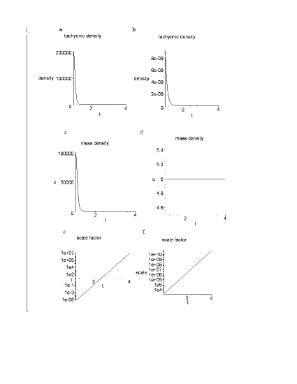
Figure 2: Inflationary scenarios: graphs on the left represent a $C>0$ model whereas graphs on the right represent a $C=0$ model. Space-time coordinates are measured in $10^{-24}$m and densities are scaled accordingly. Graphs a) and b) represent the evolution of $\alpha(t,r)$, graphs c) and d) the evolution of $\mu(t,r)$ and graphs e) and f) the increase in the scale factor (see text for explanation).

As inflation progresses, both models yield a tachyon density whose value decreases to a smaller value than $\mu(t,r)$. This value can be made small enough as not to intertfere with the physical processes that must have occured during the radiation dominated era.

The spatial geometry is again studied using the arc-length parameter, $l$, as in the matter dominated era. In this case

$$r(l)=\left\{\begin{array}[]{lll}\frac{1}{\sqrt{2C}}\left\{\left(1+4Ceb\right)^{1/2}\sin\left[2\sqrt{C}\left(l-l_{0}\right)\right]+1\right\}^{1/2}&\mbox{ for }&C>0\\ \frac{1}{\sqrt{2|C|}}\left\{\left(4|C|eb-1\right)^{1/2}\sinh\left[2\sqrt{|C|}\left(l-l_{0}\right)\right]-1\right\}^{1/2}&\mbox{ for }&C<0\\ \sqrt{\left(l-l_{0}\right)^{2}-eb}&\mbox{ for }&C=0\;.\end{array}\right.$$ (36)

Here we see that, from periodicity of the sine function, $C>0$ again can yield the closed spatial universe.

Finally, the inhomogeneity parameter in this phase is

$$I(r)={\frac{C{r}^{4}+eb}{C{r}^{4}-eb}}.$$ (37)

3 An extension to variable Lambda cosmology

Recent experiments suggest that the universe is presently in an accelerating phase. If one accepts that the net mass of the universe is positive, then the present acceleration can be explained by the figure 2a alone. Thus, the choice $\Lambda>0$ must be made. In case $\Lambda>0$ is a constant, re-collapse is incompatible with acceleration. Therefore, we consider the generalization of the previous sections to the variable $\Lambda(t)$ case. This scenario has relevance in light of recent models (mainly based on supergravity considerations) which predict that the dark energy decreases and that the universe re-collapses within a time comparable to the present age of the universe (see [40] and references therein).

Time dependent fields with equation of state $p(t)\approx-\mu(t)$ have been employed in the literature to explain certain evolutionary periods requiring positive acceleration. There are also compelling reasons from particle physics for treating the cosmological term as a dynamic quantity (see [41], [42], [43] [44] and references therein).

The field equations (3a), (3b), (3c) formally remain the same with the exception that $\Lambda=\Lambda(t)$. However, the conservation equation (4a) needs to be augmented by an additional term. The definitions of the matter, radiation and inflationary phases are retained exactly as before. Therefore, the equations for $g(r)$ in all three phases remain intact.

The solutions for $g(r)$ can be summarized as:

$$eg(r)=(\epsilon-C)r^{2}+\frac{eb}{r^{\nu}},$$ (38)

with

$$\nu=\left\{\begin{array}[]{lll}0&\mbox{ for the matter phase}\\ 2/5&\mbox{ for the radiation phase }\\ 2&\mbox{ for the inflationary phase }.\end{array}\right.$$ (39)

The three-geometries are specified as

$$d\sigma^{2}=\frac{dr^{2}}{1-Cr^{2}+\frac{eb}{r^{\nu}}}+r^{2}\,d\theta^{2}+r^{2}\sin^{2}\theta\,d\phi^{2},$$ (40)

$$\tilde{R}_{\hat{r}\hat{\theta}\hat{r}\hat{\theta}}= C+\frac{\nu eb}{2r^{\nu+2}},$$ (41a)

$$\tilde{R}_{\hat{\theta}\hat{\phi}\hat{\theta}\hat{\phi}}= C-\frac{eb}{2r^{\nu+2}},$$ (41b)

from which one obtains

$$I(r)=\frac{2Cr^{\nu+2}+\nu eb}{2\left[Cr^{\nu+2}-eb\right]}.$$ (42)

The field equations are

$$8\pi\mu(t,r)+\Lambda(t) =\frac{1}{a^{2}(t)}\left\{3\left[\dot{a}^{2}(t)+C\right]+\frac{\left(\nu-1\right)eb}{r^{\nu+2}}\right\},$$ (43a)

$$8\pi p(t,r)-\Lambda(t) =-\frac{1}{a^{2}(t)}\left\{2a(t)\ddot{a}(t)+\dot{a}^{2}(t)+C+\frac{\nu eb}{2r^{\nu+2}}\right\}.$$ (43b)

$$8\pi\alpha(t,r) =\frac{\left(\nu+2\right)eb}{2r^{\nu+2}a^{2}(t)},$$ (43c)

with conservation laws:

$$\mu(t,r)_{,t}+\frac{\dot{\Lambda}(t)}{8\pi}+H(t)\left\{3\left[\mu(t,r)+p(t,r)\right]+\alpha(t,r)\right\} =0,$$ (44a)

$$\left[p(t,r)+\alpha(t,r)\right]_{,r}+\frac{\left(\nu+2\right)eb}{8\pi r^{\nu+3}a^{2}(t)} =0.$$ (44b)

The dynamical quantities are given by

$$\ddot{a}(t)=-\left\{\frac{4\pi}{3}\left[\mu(t,r)+\alpha(t,r)+3p(t,r)\right]a(t)\right\}+\frac{1}{3}\Lambda(t)a(t).$$ (45)

The Hubble parameter and the deceleration parameter are furnished as

$$H^{2}(t)= \frac{8\pi}{3}\mu(t,r)+\frac{\Lambda(t)}{3}-\frac{C}{a^{2}(t)}-\frac{(\nu-1)eb}{3r^{\nu+2}a^{2}(t)},$$ (46a)

$$H^{2}(t)\left[2q(t)-1\right]= 8\pi p(t,r)-\Lambda(t)+\frac{1}{a^{2}(t)}\left[C+\frac{\nu eb}{2r^{\nu+2}}\right].$$ (46b)

As far as experimental evidences are concerned, the matter domain is the most relevant. Therefore, the maximum information possible will be elicited from the field equations for that domain. Setting $p(t,r)=\nu=0$ and integrating (43b) yields the “energy” conservation equation:

$$\frac{1}{2}\dot{a}^{2}(t)-\frac{1}{6a(t)}\int_{t_{2}}^{t}\Lambda(\tau)\,d[a^{3}(\tau)]-\frac{M_{0}}{a(t)}=-\frac{C}{2}.$$ (47)

Again $M_{0}$ arises from the integration and represents the total effective mass of the universe. Furthermore, $t_{2}$ is another constant representing the beginning of the matter phase. In terms of the matter fields, the mass is:

$$M_{0}= \mu(t,r)\left[\frac{4}{3}\pi a^{3}(t)\right]+\frac{eb}{6r^{2}}a(t)+\frac{a^{3}(t)}{6}\Lambda(t)-\frac{1}{6}\int_{t_{0}}^{t}\Lambda(\tau)\,d\left[a^{3}(\tau)\right],$$ (48a)

$$= \left[\mu(t_{2},r)+\alpha(t_{2},r)\right]\left[\frac{4}{3}\pi a^{3}(t_{2})\right]+\frac{a^{3}(t_{2})}{6}\Lambda(t_{2}).$$ (48b)

Here, a possible interpretation is that the first term represents the total mass of observed matter (“normal” matter), the second term the tachyonic contribution to the dark matter (non-baryonic mass for pressure, “dark energy” for tension) and the third gives rise to potential “dark energy” responsible for acceleration.

The acceleration is provided by (45) and (47) as:

$$\ddot{a}(t)= -\frac{M_{0}}{a^{2}(t)}+\frac{1}{2}\Lambda(t)a(t)-\frac{1}{6a^{2}(t)}\int_{t_{2}}^{t}\Lambda(\tau)\,d\left[a^{3}(\tau)\right]$$

$$= -\left\{\frac{\left[\mu(t,r)+\alpha(t,r)\right]\left[\frac{4}{3}\pi a^{3}(t)\right]}{a^{2}(t)}\right\}+\frac{1}{3}\Lambda(t)a(t).$$ (49)

In case $\mu(t,r)>0$, $eb>0$ and $\Lambda(t)>0$, the above terms on the right hand side produce a combination of both attractive and repulsive forces.

The Hubble parameter in the matter domain is provided by:

$$H^{2}(t)= \frac{8}{3}\pi\left[\mu(t,r)+\alpha(t,r)\right]+\frac{\Lambda(t)}{3}-\frac{C}{a^{2}(t)}$$ (50a)

$$= \frac{2M_{0}}{a^{3}(t)}-\frac{C}{a^{2}(t)}+\frac{1}{3a^{3}(t)}\int_{t_{2}}^{t}\Lambda(\tau)\,d\left[a^{3}(\tau)\right].$$ (50b)

The deceleration parameter in this domain is

$$H^{2}(t)\left[2q(t)-1\right]=\frac{C}{a^{2}(t)}-\Lambda(t).$$ (51)

It is clear from (51) that $q$ can be positive, negative or zero depending on the values of $C$ and $\Lambda(t)$. A specific model will be proposed which accommodates a spatially closed, re-collapsing universe with an accelerating period in the matter domain. In the cosmology presented here, this may be realized by setting $\Lambda(t_{2})>0$, $C>0$ and $eb>0$. Observations indicate that $C$ has a value very close to zero. A $C\leq 0$ universe has cubic divergent volume at all times save the origin when the volume is zero. If, however, $C$ is extremely small yet positive, one has finite large volume in the matter domain without contradicting observations.

The time periods for inflation, radiation and matter dominated eras are $[\epsilon,t_{1}]$, $[t_{1},t_{2}]$ and $[t_{2},T/2]$ respectively. The time $T/2$ indicates the initiation of re-collapse and thus represents the half-life of the universe. Of course, the boundaries separating the domains are not sharp as we have indicated and therefore the above simply represents a rough guideline.

A possible evolutionary scenario is depicted in figure 3. Here we plot both the scale factor $a(t)$ and cosmological term $\Lambda(t)$ as a function of cosmic time. The scale factor increases greatly during the inflationary phase (in the model presented in the figure, the inflation is driven by some matter field, not the cosmological term). This is followed by a decelerating phase and, near the present time, a period of acceleration follows. This scenario is based on the tachyonic positive pressure model and therefore this acceleration is $\Lambda$ driven. To allow for re-collapse, the cosmological term decays (starting at $t=t_{3}$) so that $\ddot{a}(t)$ becomes negative causing deceleration and eventual re-collapse. The figure is symmetric about $T/2$. Furthermore, one may have a cyclic universe where the scenario repeats after the “big crunch”.

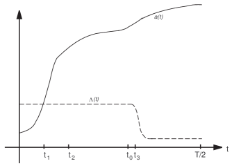
Figure 3: A possible scenario for the evolution of the universe. The present time is denoted by $t=t_{0}$ and the half-life of the universe denoted by $t=T/2$. The solid line represents the qualitative evolution of the scale factor and the dashed line the cosmological term.

A suitable $\Lambda(t)$ function may be defined by

$$\Lambda(t)=\left\{\begin{array}[]{llll}\Lambda_{0}\;\;\;\mbox{a positive constant}&\mbox{ for }&0\leq t<t_{1}\\ \Lambda_{0}&\mbox{ for }&t_{1}\leq t<t_{2}\\ \Lambda_{0}&\mbox{ for }&t_{2}\leq t<t_{3}\\ \Lambda_{0}-\epsilon_{2}(t-t_{3})^{2}+\epsilon_{4}(t-t_{4})^{4}&\mbox{ for }&t_{3}<t<T/2\;,\end{array}\right.$$ (52)

with $\epsilon_{2}>0$ and $\epsilon_{4}>0$.

The expansion factor for this case is given by:

$$a(t)=\left\{\begin{array}[]{lll}\sqrt{\frac{C}{\beta_{0}}}\cosh(\sqrt{\beta_{0}}t)&\mbox{ for }0\leq t<t_{1}\\ \sqrt{\frac{3C}{2\Lambda_{0}}+\kappa_{1}\exp\left[2\sqrt{\frac{\Lambda_{0}}{3}}t\right]+\kappa_{2}\exp\left[-2\sqrt{\frac{\Lambda_{0}}{3}}t\right]}&\mbox{ for }t_{1}\leq t<t_{2}\\ f^{-1}(t-t_{2})&\mbox{ for }t_{2}\leq t<t_{3}\;,\end{array}\right.$$ (53)

$f(a):=\int_{a(t_{2})}^{a(t)}\frac{dx}{\sqrt{\frac{\Lambda_{0}}{3}x^{2}+\left[2M_{0}-\frac{\Lambda_{0}}{3}a^{3}(t_{2})\right]x^{-1}-C}}$. There are enough arbitrary parameters in (53) so that $a(t)$ can be joined smoothly in the three phases if one wishes to enforce sharp boundaries between the phases.

The function $a(t)$ satisfies the formidable integro-differential equation

$$\left[\dot{a}(t)\right]^{2}-\frac{\Lambda_{0}}{3}a^{2}(t)-\frac{2M_{0}-\Lambda_{0}a^{3}(t)}{a(t)}+\frac{1}{3a(t)}\int_{t_{3}}^{t}\left(\epsilon_{2}\tau^{2}-\epsilon_{4}\tau^{4}\right)f\left[a^{3}(\tau)\right]=0$$ (54)

in the interval $t_{3}\leq t<T/2$. The above equation is too difficult to solve analytically at this stage.

The spatial geometry for $C>0$ is governed by $r(l)$ as

$$d\sigma^{2}=dl^{2}+r^{2}(l)\left(d\theta^{2}+\sin^{2}\theta\,d\phi^{2}\right),$$ (55)

$$r(l)=\left\{\begin{array}[]{lll}\frac{1}{\sqrt{2C}}\left\{\left(1+4Ceb\right)^{1/2}\sin\left[2\sqrt{C}\left(l-l_{0}\right)\right]+1\right\}^{1/2}&\mbox{ for inflation}\\ F^{-1}\left(l-l_{0}\right)&\mbox{ for radiation}\\ \sqrt{\frac{1+eb}{2C}}\sin\left[\sqrt{C}\left(l-l_{0}\right)\right]&\mbox{ for matter}\;.\end{array}\right.$$ (56)

Here, $F(r):=\int\frac{dr}{\sqrt{1-Cr^{2}+eb/r^{2/5}}}\>$. By previous discussions, in all phases the physical universes are closed. Moreover, the total volume corresponding to the three dimensional spatial sub-manifold in the matter phase is given by

$$\frac{2\pi\left(1+eb\right)}{C}\left[a(t_{0})\right]^{3}\int_{l_{0}}^{l_{0}+\pi/\sqrt{C}}\sin^{2}\left[\sqrt{C}\left(l-l_{0}\right)\right]\,dl=\frac{\pi^{2}\left(1+eb\right)}{C^{3/2}}\left[a^{3}(t_{0})\right],$$ (57)

(Note that in the limit $C\rightarrow 0_{+}$, the above volume diverges).

We now wish to address the singularity at $r=0$. The two dimensional geometries (restricted to $\theta=\pi/2$) yield:

$$d\sigma_{2}^{2}=\frac{dr^{2}}{1-Cr^{2}+\frac{eb}{r^{\nu}}}+r^{2}\,d\phi^{2}.$$ (58)

These two-dimensional surfaces embedded in a three-dimensional Euclidean space possess the following Gaussian curvatures:

$$K(r,\phi)=\left\{\begin{array}[]{lll}C+\frac{eb}{r^{4}}\;\;>0&\mbox{ for inflation}\\ C+\frac{eb}{5r^{12/5}}\;\;>0&\mbox{ for radiation}\\ C\;\;>0&\mbox{ for matter}\;.\end{array}\right.$$ (59)

In the matter domain, the surface is locally isometric to a spherical surface of radius $1/\sqrt{C}$. However, the original three dimensional spaces in the equation (41b) all exhibit a singularity at the limit $r\rightarrow 0_{+}$. Therefore, some possible global pictures for these three dimensional spaces are provided in figure 4.

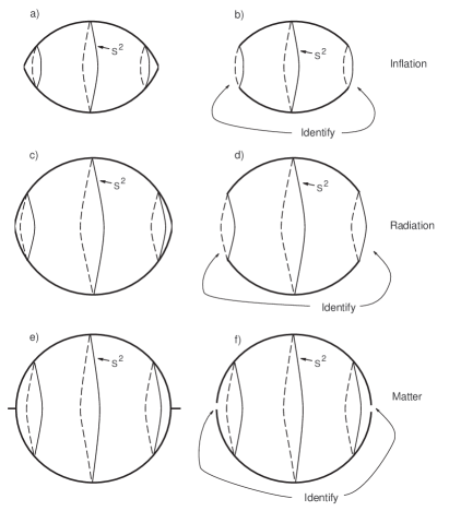
Figure 4: Possible global pictures for spatial sections in the inflationary (a, b), radiation (c, d) and matter (e, f) dominated eras. The diagrams on the left include the points corresponding to $r=0$. The diagrams on the right have a neighborhood about $r=0$ removed and the boundaries identified. Note that in the matter domain the surfaces are isometric to spheres yet singularities still exist at $r=0$ as indicated by the “hairs” in diagram e.

In the figure 4, one of the angles is suppressed so that latitudinal lines represent two-spheres. Two possible scenarios exist; the figures on the left represent the spatial manifold for inflation, radiation dominated and matter dominated eras which include $r=0$ (the left and right points in each figure). The figures on the right have the domains in the neighborhood of $r=0$ excised. The left and right boundaries are therefore identified. Note that as the evolution progresses, the anisotropy of the spatial sections diminishes yielding a sphere in the matter domain. This is therefore quite compatible with observation. The poles of the sphere, however, are singular or must be excised. The singularity appears to be “soft” in that it is of the conical type. Also, the equations, being local, are valid in a domain $r_{1}<r<r_{2}$ which need not include $r=0$. It is likely that such a singularity would be absent in a quantum theory of gravity which would be manifest at high energies.

4 Compatibility with current observations

Current observations indicate a universe which is approximately 5% baryonic matter, 20% non-baryonic matter and 75% “dark energy” which is responsible for the recent acceleration phase. The “directly” measurable quantities in cosmology are $\mu(t,r)$, $H$ and $q_{0}$. Roughly, in the present epoch (and, as we are dealing with an inhomogeneous universe, in our neighborhood of the universe) these quantities possess the following approximate values:

$$\mu(t_{0},r_{0})\approx 1.6\times 10^{-56}\,\mbox{m}^{-2},$$ (60a)

$$H^{2}:= \left[\frac{\dot{a}(t)}{a(t)}\right]^{2}\approx 7.3\times 10^{-53}\,\mbox{m}^{-2},$$ (60b)

$$q_{0}\approx -0.4\;\;\;.$$ (60c)

Here $t_{0}$ and $r_{0}$ are the current time and position respectively.

The deceleration equation (15c) provides a relationship (using the above parameters along with (14c)) between $\Lambda$ and $\alpha(t,r)$ (we assume that any time variation in $\Lambda$ can be ignored):

$$\alpha(t_{0},r_{0})=\left(8.0\times 10^{-2}\Lambda-6.9\times 10^{-54}\right)\mbox{m}^{-2}\;.$$ (61)

If there is no cosmological constant, then the second term in this equation indicates the approximate value the tachyon tension must possess in our region of the universe to drive the observed acceleration.

If, on the other hand, the tachyon possesses positive pressure (contributing all or in part to the non-baryonic dark matter of the universe) then the acceleration is $\Lambda$ driven. In such a case $\alpha(t_{0},r_{0})$ may take on the following values:

$$0\leq\alpha(t_{0},r_{0})\lesssim 4\mu(t_{0},r_{0})\approx 6.4\times 10^{-56}\,\mbox{m}^{-2}.$$ (62)

The upper limit comes from noting the observational evidence that the dark matter contribution is approximately four times the baryonic contribution to the matter content. This sets a restriction on the cosmological constant to be of the order

$$\Lambda=\mathcal{O}\left(10^{-52}\right)m^{-2}.$$ (63)

Alternately we may begin the analysis by using equation (51) and solving for $\Lambda$ (with the parameters quoted above)

$$\Lambda_{0}=\frac{C}{a^{2}(t)}-H^{2}\left(2q-1\right)=\frac{C}{a^{2}(t)}+13.14\times 10^{-53}.$$ (64)

Also, by equation (50a), we may write

$$3H^{2} = 8\pi\left[\mu(t,r)+\alpha(t,r)\right]+\Lambda_{0}-\frac{3C}{a^{2}(t)}$$

$$2.19\times 10^{-52} = 8\pi\left[\mu(t,r)+\alpha(t,r)\right]+1.31\times 10^{-52}-2\frac{C}{a^{2}(t)}$$ (65)

(in the last equation (64) has been used.) Isolating the $\mu(t,r)+\alpha(t,r)$ term and using in (48a) yields

$$\frac{M_{0}}{\frac{4\pi}{3}a^{3}(t_{0})}=3.48\times 10^{-54}+\frac{1}{8\pi}\left[\frac{C}{a^{2}(t_{0})}+1.3\times 10^{-52}\right]\left[\frac{a(t_{2})}{a(t_{0})}\right]^{3}+\frac{C}{4\pi a^{2}(t_{0})}.$$ (66)

The $C/a^{2}(t)$ terms represent the present “radius”-squared of the universe. The left hand side of (66) is an analogue of the present Newtonian density of the universe. The above equation is therefore useful in determining the radius of the universe given the density or vice-versa.

5 Concluding remarks

This paper considers a simple cosmological model consisting of perfect fluid matter supplemented with a “tachyonic dust”. The perfect fluid, with positive mass density, makes up the ordinary matter as in the standard cosmology. The tachyonic dust term is a source of pressure which, interestingly, can increase the effective mass of the universe. In this case it could potentially be utilised as a source of dark matter although the clustering properties need to be studied. In case the tachyonic dust term is a source of tension, it may be responsible for the observed recent acceleration of the universe. This model provides the simplest pressure enhancing extension to the successful FLRW scenario. At late times, the solution generates a geometry compatible with FLRW.

References

[1]
G. Lemaître,
Ann. Soc. Sci. BruxellesA53 (1933) 51. Engl.
trans. Gen. Rel. Grav.29 (1997) 641.
[2]
R. C. Tolman,
Proc. Nat. Acad. Sci. USA20 (1934) 169. Reprint
Gen. Rel. Grav.29 (1997) 935.
[3]
C. Misner,
Astrophys. J.151 (1968) 431.
[4]
A. Krasiński,
Inhomogeneous Cosmological Models (Cambridge University
Press, Cambridge, 1997).
[5]
A. Feinstein, J. Ibáñez and P. Labraga,
J. Math. Phys.36 (1995) 4962.
[6]
J. Ibáñez and I. Olasagasti,
J. Math. Phys.37 (1996) 6283.
[7]
J. D. Barrow and K. E. Kunze,
gr-qc/9611007.
[8]
J. D. Barrow and K. E. Kunze,
Phys. Rev.D56 (1997) 741.
[9]
J. Ibáñez and I. Olasagasti,
Class. Quant. Grav.15 (1998) 1937.
[10]
A. Krasiński,
Proceedings of the 49th Yamada Conference on black holes and high-energy
astrophysics Kyoto, Japan, (Universal Academic Press, Tokyo,
1998)
[11]
J. D. Barrow and R. Maartens,
Phys. Rev.D59 (1999) 043502.
[12]
J. V. Arnau, M. Fullana, L. Monreal and D. Sáez,
Astroph. J.402 (1993) 359.
[13]
D. Sáez, J. V. Arnau and M. Fullana,
Mon. Not. Roy. Astr. Soc.263 (1993) 681.
[14]
J. V. Arnau, M. Fullana and D. Sáez,
Mon. Not. Roy. Astr. Soc.268 (1994) L17.
[15]
M. Fullana, J. V. Arnau, and D. Sáez,
Mon. Not. Roy. Astr. Soc.280 (1996) 1181.
[16]
A. Mazumdar, S. Panda, A. Pérez-Lorenzana,
Nucl. Phys.B614 (2001) 101.
[17]
A. Sen,
J. H. E. P.0204 (2002) 048.
[18]
G. W. Gibbons,
Phys. Let.B537 (2002) 1.
[19]
T. Padmanabhan,
Phys. Rev.D66 (2002) 021301.
[20]
A. Feinstein,
Phys. Rev. D 66 (2002) 063511.
[21]
A. Frolov, L. Kofman and A. Starobinsky,
Phys. Lett.B545 (2002) 8.
[22]
L. Kofman and A. Linde,
J. H. E. P.0207 (2002) 004.
[23]
P. Matlock, R. C. Rashkov, K. S. Viswanathan and Y. Yang,
Phys. Rev.D66 (2002) 026004.
[24]
M. Sami, P. Chingangbam and T. Qureshi,
Phys. Rev.D66 (2002) 043530.
[25]
X. Li, D. Liu and J. Hao,
hep-th/0207146.
[26]
J. S. Bagla, H. K. Jassal and T. Padmanabhan,
astro-ph/0212198.
[27]
D. Choudhury, D. Ghoshal, D. P. Jatkar and S. Panda,
Phys. Let.B544 (2003) 231.
[28]
C. Kim, H. B. Kim and Y. Kim,
Phys. Let.B552 (2003) 111.
[29]
G. W. Gibbons,
hep-th/0301117.
[30]
A. Das and D. Kay,
Can. J. Phys.66 (1988) 1031.
[31]
A. G. Reiss, et al,
Astron. J.116 (1998) 1009.
[32]
S. Perlmutter, et al,
Astrophys. J.517 (1999) 565.
[33]
M. K. Mak and T. Harko,
Proc. Roy. Soc. Lond.A459 (2003) 393.
[34]
B. V. Ivanov,
Phys. Rev.D65 (2002) 104011.
[35]
K. Dev and M. Gleiser,
Gen. Rel. Grav.34 (2002) 1793.
[36]
A. G. Reiss, et al,
Astrophys. J.560 (2001) 49.
[37]
G. Lemaitré,
Ann. Soc. Sci. Brux.A47 (1927) 49.
[38]
A. S. Eddington,
Mon. Not. Roy. Astron. Soc.90 (1930) 668.
[39]
R. Brandenberger,
Proceedings of the International School on
Cosmology Kish Island, Iran, (Kluwer, Dordrecht, 2000).
[40]
R. Kallosh and A. Linde,
J. Cosmol. Astropart. Phys.02 (2003) 002.
[41]
P. G. Bergmann,
Int. J. Theor. Phys.1 (1968) 25.
[42]
R. V. Wagoner,
Phys. Rev.D1 (1970) 3209.
[43]
A. D. Linde,
JETP Let.19 (1974) 183.
[44]
J. M. Overduin and F. I. Cooperstock,
Phys. Rev.D58 (1998) 043506.