Stockholm
USITP 03-03
April 2003

The Hessian of the entropy function can be thought of as a metric tensor on the state space. In the context of thermodynamical fluctuation theory Ruppeiner has argued that the Riemannian geometry of this metric gives insight into the underlying statistical mechanical system; the claim is supported by numerous examples. We study this geometry for some families of black holes. It is flat for the BTZ and Reissner–Nordström black holes, while curvature singularities occur for the Reissner–Nordström–anti–de Sitter and Kerr black holes.

1. Introduction

It has been argued that the Hessian of the thermodynamic entropy function S, that is the matrix

$$g_{ij}\equiv-\partial_{i}\partial_{j}S(X)\ ,$$ (1)

can be thought of as a Riemannian metric on the state space in a meaningful way. We will refer to it as the Ruppeiner metric. It is clearly assumed that the coordinates $X^{i}$ form some preferred affine space; in ordinary thermodynamics they are chosen to be the extensive variables of the system. In this paper we will study this geometry for some important families of black holes, choosing the conserved charges $M$, $J$ and $Q$ as coordinates. The idea is that the Riemannian curvature in some sense measures the complexity of the underlying statistical mechanical model, which in this case is unknown but may well be in the process of being uncovered by progress in quantum gravity. The results are rather pleasing: We will find that the BTZ and Reissner–Nordström families have a flat thermodynamic geometry, while the Reissner–Nordström–anti-de Sitter and Kerr families exhibit curvature singularities.

Our belief that this is a meaningful result rests on an analogy to thermodynamic fluctuation theory, where a similar claim was originally based simply on the observation that the thermodynamic geometry of the ideal gas is flat [1]. Let us recall the argument: Let $W$ be the number of (equiprobable) microstates consistent with a given macroscopical state. Boltzmann argued that the macroscopic entropy is given by

$$S=k\ln{W}\ .$$ (2)

Einstein rewrote this equation as

$$P\propto e^{\frac{1}{k}S}\ ,$$ (3)

where $P$ is the probability that the given macrostate will be realized. We can Taylor expand the entropy around an equilibrium state, taking into account that the entropy has a maximum there, and introduce the Hessian matrix

$$g_{ij}\equiv-\partial_{i}\partial_{j}S(X)\ .$$ (4)

Here $X$ stands for the $n$ extensive variables shifted so that they take the value zero at equilibrium. The matrix is positive definite if the entropy is concave. If we normalize the resulting probability distribution (and set $k=1$) we obtain

$$P(X)=\frac{\sqrt{g}}{(2{\pi})^{\frac{n}{2}}}e^{-\frac{1}{2}g_{ij}X^{i}X^{j}}$$ (5)

as the probability distribution governing fluctuations around the equilibrium state. The pair correlation functions are then given by the contravariant metric tensor,

$$\langle X^{i}X^{j}\rangle=g^{ij}\ .$$ (6)

In the derivation we assume that the fluctuations are small. So far everything is standard [2]. It is important to realize that the physical situation here is a system described by the canonical (or grand canonical) ensemble, and moreover that one extensive parameter (typically the volume) has been set aside and used to give an appropriate physical dimension to $g_{ij}$. If this is not done the Gibbs–Duhem relation will imply that $g_{ij}$ has a null eigenvector.

Ruppeiner [3] argues that the Riemannian geometry of the metric tensor $g_{ij}$ carries information about the underlying statistical mechanical model of the system. In particular he argues that the metric is flat if and only if the statistical mechanical system is non–interacting, while curvature singularities are a signal of critical behaviour—more precisely of divergent correlation lengths. This viewpoint has received support from various directions [4] [5] [6]. Evidently the construction is related to the Fisher–Rao metric that is used in mathematical statistics, although it is fair to add that the Riemannian geometry of the Fisher–Rao metric does not play any significant role there—statistical geometry is rather more subtle [7].

The reason why Ruppeiner’s arguments do not apply directly to black holes is that the thermodynamics of black holes exhibit some unfamiliar features which are in fact generic to systems with long range interactions in general, and to self–gravitating systems in particular [8]. First we encounter negative specific heats, that is to say that the entropy is not a concave function. Second there are no extensive variables. Technically this means that the Ruppeiner metric will not be positive definite; on the other hand it will not have any null eigenvectors either. But it also means that the canonical ensemble does not exist, and that it is difficult to choose a physical dimension for the metric. Nevertheless we believe that the Ruppeiner geometry of black holes is telling us something; our justification is mainly the a posteriori one that once it has been worked out for some examples we will find an interesting pattern. For some further observations on the role of the Ruppeiner metric in black hole physics see Ferrara et al. [9]. For background information on black hole thermodynamics see Davies [10].

Some technical comments before we begin: Although the definition of the Ruppeiner metric depends on a preferred affine coordinate system we can afterwards transform ourselves to any coordinate system that we find convenient. Here we take note of a related construction due to Weinhold [11], who defined a metric in the energy representation through

$$g^{W}_{ij}\equiv\partial_{i}\partial_{j}M(S,N^{a})\ .$$ (7)

We use $M$ to denote energy and $N^{a}$ to denote any other extensive variables. The entropy function is naturally a function of $M$ and $N^{a}$, so that in this notation the Ruppeiner metric is

$$g_{ij}=-\partial_{i}\partial_{j}S(M,N^{a})\ .$$ (8)

Of course we can transform the Ruppeiner metric to the coordinate system used to define the Weinhold metric, and conversely. Interestingly the two metrics are conformally related [12] [4]:

$$ds^{2}=g_{ij}dM^{i}dM^{j}=\frac{1}{T}g^{W}_{ij}dS^{i}dS^{j}\ ,$$ (9)

where $M^{i}=(M,N^{a})$, $S^{i}=(S,N^{a})$ and $T$ denotes the temperature

$$T=\frac{\partial M}{\partial S}\ .$$ (10)

Eq. (9) often provides the most convenient way to compute the Ruppeiner metric.

The organization of paper is as follows: In section 2 we consider the Reissner–Nordström and Reissner–Nordström–anti-de Sitter black holes in some detail. In section 3 we give a briefer treatment of the Kerr and BTZ black holes, and make some brief observations on the three dimensional Kerr–Newman family. Our conclusions are in section 4.

2. Reissner–Nordström black holes.

We will describe one case in full detail, and we choose the Reissner–Nordström family of black holes for this purpose. They are spherically symmetric black holes carrying mass $M$ and charge $Q$. The event horizon is ruled by a Killing vector field whose norm is

$$||{\xi}||^{2}=-\frac{1}{r^{2}}\left(\frac{r^{4}}{l^{2}}+r^{2}-2Mr+Q^{2}\right)\ ,$$ (11)

where $r$ is a natural radial coordinate chosen so that the area of a sphere at constant $r$ equals $4{\pi}r^{2}$. For later reference we have included a negative cosmological constant

$${\lambda}=-\frac{3}{l^{2}}$$ (12)

but for the time being we set ${\lambda}=0$, in which case the polynomial defining $||{\xi}||^{2}$ has two roots $r_{+}$ and $r_{-}$. These values of $r$ characterize the outer and inner event horizons, respectively. We find that

$$M=\frac{1}{2}(r_{+}+r_{-})\hskip 22.76219ptQ^{2}=r_{+}r_{-}\hskip 22.76219ptS=r_{+}^{2}\ ,$$ (13)

where the entropy is one quarter of the area of the event horizon times Boltzmann’s constant,

$$S=\frac{k}{4}A=k{\pi}r_{+}^{2}=r_{+}^{2}\ ,$$ (14)

and we exercised our right to set $k=1/{\pi}$. The extremal limit, beyond which the singularity becomes naked, occurs when the root $r_{+}$ is a double root. This happens at

$$Q^{2}=M^{2}\hskip 14.22636pt\Leftrightarrow\hskip 14.22636pt\frac{Q^{2}}{S}=1\ .$$ (15)

The thermodynamics of these black holes is now defined by the fundamental relation

$$M=\frac{\sqrt{S}}{2}\left(1+\frac{Q^{2}}{S}\right)\ .$$ (16)

This is in the energy representation, which proves to be the most convenient one here—the Ruppeiner metric becomes quite unwieldy when expressed in terms of its natural coordinates.

The Hawking temperature is

$$T=\frac{\partial M}{\partial S}=\frac{1}{4\sqrt{S}}\left(1-\frac{Q^{2}}{S}\right)$$ (17)

and the electric potential is given by

$${\Phi}=\frac{\partial M}{\partial Q}=\frac{Q}{\sqrt{S}}\ .$$ (18)

In its natural coordinates the Weinhold metric becomes

$$ds^{2}_{W}=\frac{1}{8S^{\frac{3}{2}}}\left(-\left(1-\frac{3Q^{2}}{S}\right)dS^{2}-8QdQdS+8SdQ^{2}\right)\ .$$ (19)

We observe that the component $g^{W}_{SS}$ vanishes and changes sign at

$$\frac{Q^{2}}{S}=\frac{1}{3}\ .$$ (20)

This implies that the specific heat $C_{Q}$ diverges and changes sign there. In ref. [10] Davies argued that this implies that the system is undergoing a phase transition. We will see that this is not so—nothing special happens to the convexity of the energy function at this point.

It is essential to use the coordinates $S,Q$ in the definition of the Weinhold metric. But once we have it it is convenient to introduce the new coordinate

$$u=\frac{Q}{\sqrt{S}}\ ;\hskip 22.76219pt-1\leq u\leq 1\ .$$ (21)

The limits on the coordinate range are set by the fact that the black hole becomes extremal there. We now find that

$$ds^{2}_{W}=\frac{1}{8S^{\frac{3}{2}}}\left(-(1-u^{2})dS^{2}+8S^{2}du^{2}\right)\ .$$ (22)

This is on diagonal form.

In these coordinates the Ruppeiner metric is given by

$$ds^{2}=\frac{1}{T}ds^{2}_{W}=-\frac{dS^{2}}{2S}+4S\frac{du^{2}}{1-u^{2}}\ .$$ (23)

This metric is flat. To see this introduce new coordinates

$${\tau}=\sqrt{2S}\hskip 22.76219pt\sin{\frac{\sigma}{\sqrt{2}}}=u\ .$$ (24)

The Ruppeiner metric now takes the form

$$ds^{2}=-d{\tau}^{2}+{\tau}^{2}d{\sigma}^{2}\ ,$$ (25)

which is recognizable as a timelike wedge in Minkowski space when described by Rindler coordinates. This seems to us to be a surprising result and provides some a posteriori justification for considering the Ruppeiner metric in the first place.

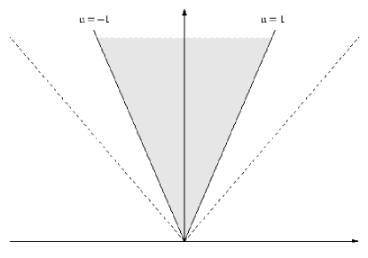
Figure 1: The state space of the Reissner–Nordström black holes shown as a wedge in a flat Minkowski space.

For completeness let us discuss the case of a non–zero and negative cosmological constant. Eq. (11) is now a quartic polynomial. The event horizon is determined by its largest positive root $r_{+}$. The entropy is still determined by one quarter of the area of the event horizon, and it is not difficult to see that the fundamental relation is given by

$$M=\frac{\sqrt{S}}{2}\left(1+\frac{S}{l^{2}}+\frac{Q^{2}}{S}\right)\ .$$ (26)

The extremal limit occurs when $r_{+}$ is a degenerate root, and this happens when

$$\frac{Q^{2}}{S}=1+\frac{3S}{l^{2}}\ .$$ (27)

The Hawking temperature is

$$T=\frac{1}{4\sqrt{S}}\left(1+\frac{3S}{l^{2}}-\frac{Q^{2}}{S}\right)\ .$$ (28)

This vanishes in the extremal limit, as it should.

The Weinhold metric is

$$ds^{2}_{W}=\frac{1}{8S^{\frac{3}{2}}}\left(-\left(1-\frac{3S}{l^{2}}-\frac{3Q^{2}}{S}\right)dS^{2}-8QdSdQ+8SdQ^{2}\right)\ .$$ (29)

It can be diagonalized using the same coordinate transformation as above, with the result that the conformally related Ruppeiner metric becomes

$$ds^{2}=\frac{1}{1+\frac{3{\tau}^{2}}{2l^{2}}-u^{2}}\left(-\left(1-\frac{3{\tau}^{2}}{2l^{2}}-u^{2}\right)d{\tau}^{2}+2{\tau}^{2}du^{2}\right)\ .$$ (30)

The geometry is non–trivial. By inspection we see that the signature of the metric—and with it the stability properties of the thermodynamic system—changes for sufficiently large black holes (using the length scale $l$ set by ${\lambda}$). This feature is of course well known—it means that the entropy function becomes concave for sufficiently large black holes [13]. The details of the thermodynamics of this case are actually quite interesting and can be found in the literature [14] [15]. Our concern is the curvature scalar of the Ruppeiner metric, which is

$$R=\frac{9}{l^{2}}\frac{\left(\frac{3S}{l^{2}}+\frac{Q^{2}}{S}\right)\left(1-\frac{S}{l^{2}}-\frac{Q^{2}}{S}\right)}{\left(1-\frac{3S}{l^{2}}-\frac{Q^{2}}{S}\right)^{2}\left(1+\frac{3S}{l^{2}}-\frac{Q^{2}}{S}\right)}\ .$$ (31)

We observe that the curvature diverges both in the extremal limit and along the curve where the metric changes signature, that is where the thermodynamical stability properties are changing.

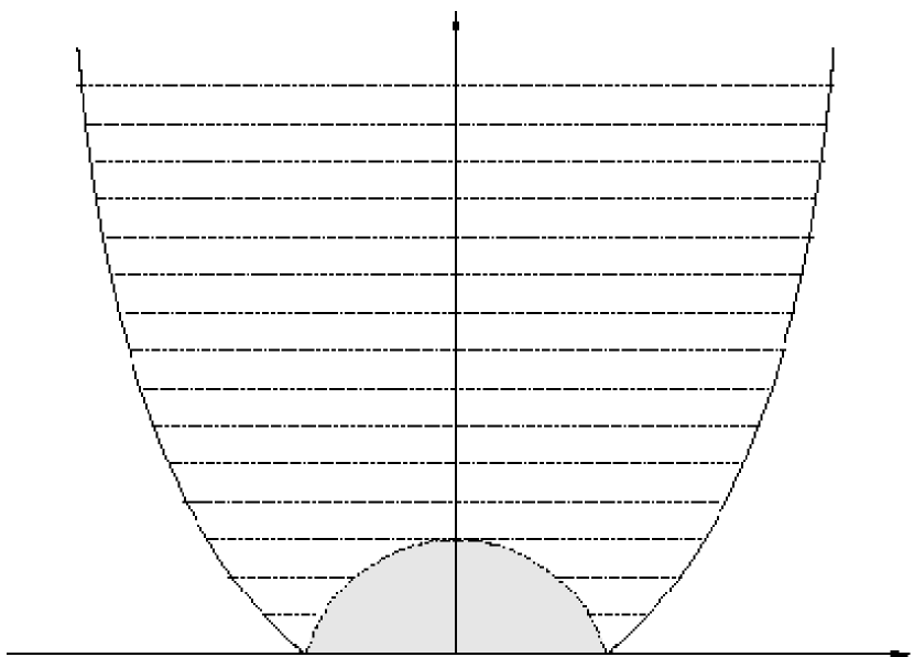
Fig.(A)

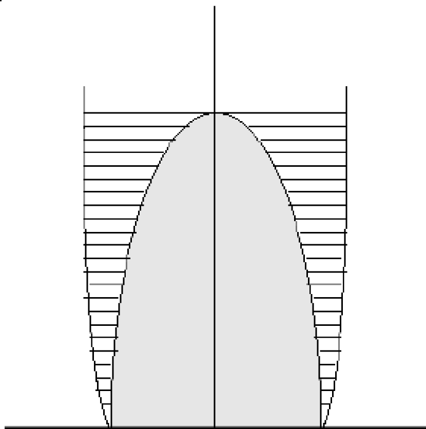
Fig.(B)

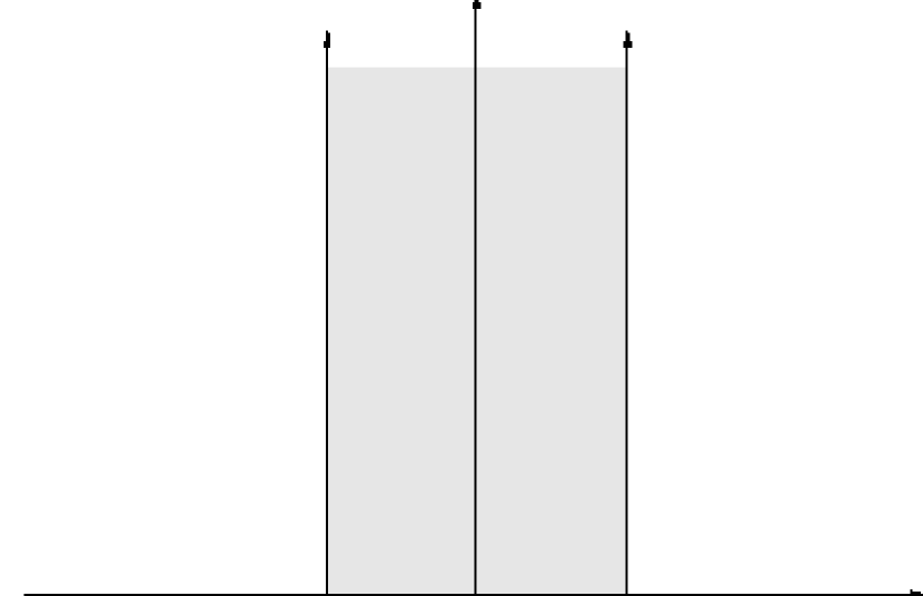
Fig.(C)

Figure 2: The state space for Reissner–Nordström–anti-de Sitter black holes; our coordinates are $u$ and $S$ and the cosmological constant decreases as we go from A to C. The grey region has a Lorentzian metric. Note that C is the same as figure 1 although the coordinates differ.

3. Other black holes.

The Reissner–Nordström black holes belong to the three parameter Kerr–Newman family of black holes, with fundamental relation

$$M=\sqrt{\frac{S}{4}+\frac{1}{S}\left(J^{2}+\frac{Q^{4}}{4}\right)+\frac{Q^{2}}{2}}\ ,$$ (32)

or in the entropy representation

$$S=2M^{2}-Q^{2}+2M^{2}\sqrt{1-\frac{Q^{2}}{M^{2}}-\frac{J^{2}}{M^{4}}}\ .$$ (33)

Here $J$ measures the spin of the black hole. If we set $Q=0$ we obtain the Kerr black holes, which are worthy of attention because they are believed to exist as physical objects. Their extremal limit is given by

$$\frac{J}{M^{2}}=\pm 1\ .$$ (34)

From our point of view it is advantageous to use the entropy representation here. The Ruppeiner metric becomes

$$ds^{2}=\frac{2}{(1-\frac{J^{2}}{M^{4}})^{\frac{3}{2}}}\left(-2\left((1-\frac{J^{2}}{M^{4}})^{\frac{3}{2}}+1-\frac{3J^{2}}{M^{4}}\right)dM^{2}-\frac{4J}{M^{3}}dMdJ+\frac{dJ^{2}}{M^{2}}\right).$$ (35)

This can be diagonalized by means of the coordinate transformation

$$v=\frac{J}{M^{2}}\ ;\hskip 22.76219pt-1\leq v\leq 1\ .$$ (36)

The Ruppeiner geometry is curved, but its curvature scalar takes a quite simple form:

$$R=\frac{1}{4M^{2}}\frac{\sqrt{1-\frac{J^{2}}{M^{4}}}-2}{\sqrt{1-\frac{J^{2}}{M^{4}}}}\ .$$ (37)

We observe that $R$ diverges in the extremal limit. It is however difficult to draw any firm conclusions from this because of the difficulty that the entropy function is not concave so that the fluctuation theory does not apply. A curious observation is that the Weinhold geometry of the Kerr black holes is actually flat.

We used the computer program Classi [16] to study the full three dimensional state space of the Kerr–Newman black holes (and to add some details to the table below). In particular, we computed the Cotton–York tensor and from this we could conclude that the Ruppeiner geometry is not conformally flat. Beyond this we did not uncover any noteworthy features.

There is one case where the thermodynamical response functions are positive throughout. This is the case of the 2+1 dimensional BTZ black holes [17]. They occur in a theory—Einstein’s equation in 2+1 dimensions with a negative cosmological constant included—that is close to trivial from a dynamical point of view, but they are bona fide black holes nevertheless. Their thermodynamics is given by the fundamental relation

$$M=S^{2}+\frac{J^{2}}{4S^{2}}\ ,$$ (38)

where we choose $k=2/{\pi}$. The extremal limit, beyond which no black hole exists because the singularity (or “singularity”, for connaisseaurs of these solutions [18]) becomes naked, is given by $J=\pm M$. It is also worth noting that $M=0$ does not correspond to the “background” anti-de Sitter spacetime but to another kind of extremal black hole.

This time the energy representation is the convenient one to use. The Weinhold metric diagonalizes if we trade $J$ for the new coordinate

$$u\equiv\frac{J}{2S^{2}}\ ;\hskip 28.45274pt-1\leq u\leq 1\ .$$ (39)

Finally the Ruppeiner metric is

$$ds^{2}=\frac{dS^{2}}{S}+\frac{Sdu^{2}}{1-u^{2}}\ .$$ (40)

This is a wedge of an Euclidean flat space described in coordinates that are polar coordinates in slight disguise.

We summarize our results in a table.

Black hole family	Ruppeiner	Weinhold
RN	Flat	Curved, no Killing vectors
RNadS	Curved, no Killing vectors	Curved, no Killing vectors
Kerr	Curved, no Killing vectors	Flat
BTZ	Flat	Curved, no Killing vectors
Kerr–Newman	Curved	Curved

4. Conclusions

In conclusion we have studied the Ruppeiner and Weinhold geometries of BTZ and Kerr–Newman black holes. In analogy to thermodynamic fluctuation theory we expect that a flat Ruppeiner geometry is a sign that an underlying statistical mechanical model must be exceptionally simple (“non–interacting”), while curvature singularities signal exceptional (“critical”) behaviour in the underlying model. We found that the Ruppeiner geometry is flat for the BTZ and Reissner–Nordström families, while the curvature diverges in the extremal limit in the Kerr and Reissner–Nordström–anti-de Sitter families. In the latter case the curvature is also singular along the line where the stability properties change. We find these results sensible, and also simpler than one would perhaps have expected. For the full Kerr–Newman family no elegant results were found.

An interesting but of course very speculative use of the Ruppeiner geometry for the Kerr family is to let the volume form serve as a Bayesian prior for the amount of spin one should expect; observations concerning this can be expected in the not too far future.

References

- [1] G. Ruppeiner, Phys. Rev. A20 (1979) 1608.
- [2] L. Landau and E. M. Lifshitz, Statistical Physics, Pergamon Press, London 1980.
- [3] G. Ruppeiner, Rev. Mod. Phys. 67 (1995) 605; 68 (1996) 313(E).
- [4] R. Mrugała, Physica 125A (1984) 631.
- [5] P. Salamon, J. D Nulton and R. S. Berry, J. Chem. Phys. 82 (1985) 2433.
- [6] D. C. Brody and A. Ritz, Geometric phase transitions, cond-mat/9903168.
- [7] N. N. Čencov, Statistical Decision Rules and Optimal Inference, Amer. Math. Soc., Providence 1982.
- [8] T. Padmanabhan, Phys. Rep. 188 (1990) 285.
- [9] S. Ferrara, G. W. Gibbons and R. Kallosh, Nucl. Phys. B500 (1997) 75.
- [10] P. C. W. Davies, Proc. R. Soc. Lond. A353 (1977) 499.
- [11] F. Weinhold, J. Chem. Phys. 63 (1975) 2479.
- [12] P. Salamon, J. D. Nulton and E. Ihrig, J. Chem. Phys. 80 (1984) 436.
- [13] S. W. Hawking and D. N. Page, Comm. Math. Phys. 87 (1983) 577.
- [14] J. Louko and S. N. Winters-Hilt, Phys. Rev. D54 (1996) 2647.
- [15] A. Chamblin, R. Emparan, C. V. Johnson and R. C. Myers, Phys. Rev. D60 (1999) 104026.
- [16] J. E. Åman, “Manual for classi: Classification Programs for Geometries in General Relativity”, ITP, Stockholm University, Technical Report, 2002. Provisional edition. Distributed with the sources for sheep and classi.
- [17] M. Bañados, C. Teitelboim and J. Zanelli, Phys. Rev. Lett. 69 (1992) 1849.
- [18] M. Bañados, M. Henneaux, C. Teitelboim and J. Zanelli, Phys. Rev. D48 (1993) 1506.