The accelerated expansion of the Universe as a quantum cosmological effect

Abstract

We study the quantized Friedmann-Lemaître-Robertson-Walker (FLRW) model minimally coupled to a free massless scalar field. In a previous paper, fab2 , solutions of this model were constructed as gaussian superpositions of negative and positive modes solutions of the Wheeler-DeWitt equation, and quantum bohmian trajectories were obtained in the framework of the Bohm-de Broglie (BdB) interpretation of quantum cosmology. In the present work, we analyze the quantum bohmian trajectories of a different class of gaussian packets. We are able to show that this new class generates bohmian trajectories which begin classical (with decelerated expansion), undergo an accelerated expansion in the middle of its evolution due to the presence of quantum cosmological effects in this period, and return to its classical decelerated expansion in the far future. We also show that the relation between luminosity distance and redshift in the quantum cosmological model can be made close to the corresponding relation coming from the classical model suplemented by a cosmological constant, for $z<1$. These results suggest the posibility of interpreting the present observations of high redshift supernovae as the manifestation of a quantum cosmological effect.

I Introduction

Recent measurements of high redshift supernovae SN1 SN indicate that the Universe is presently in accelerated expansion and not in a decelerated one, as was firmly believed by cosmologists since Hubble’s observation and its interpretation in the framework of General Relativity (GR). This was a spectacular break through in our understanding (or misunderstanding) of the Universe, and it became a major task to Cosmology and Astrophysics to explain this unexpected fact. Staying in the domain of classical GR and, consequently, considering the Friedmann’s equations as valid, the only way to explain such present acceleration of the Universe is by considering the existence of some negative pressure dark energy SN1 triangle garnavich wang .This cosmic dark energy opposes the self-atraction of matter and is causing the expansion of the universe to be positively acceleratedtriangle . The most obvious candidate to be such dark energy is the cosmological constant and/or the vacuum quantum fluctuations of fields, which do have negative pressure. However, theorists estimates that the zero point energies of the quantum fields must be at least 55 orders of magnitude larger than the critical density value. Hence, there must exist some yet unknown profound theoretical reason for the many contributions to the effective value of the cosmological constant be cancelled out to yield a number 55 orders of magnitude less then expected, or even zero. This is known as the cosmological constant problem. Some theorists believe that some profound symmetry requirements can be found to explain an exact cancellation, but not a partial one with an extreme fine tuning. In the case where the effective cosmological constant is indeed exactly zero, there were proposed some candidates in order to explain the present accelerated expansion of the Universe as, for example, a very light, evolving scalar field called quintescence quint jer .

Another way to tackle this problem is by considering that presently, at cosmological scales, classical GR is not valid. In other words, instead of changing the right-hand-side (RHS) of Einstein’s equations by introducing some new negative pressure fluid, one could try to find physical reasons which justify the modification of its left-hand-side (LHS) accordingly. How this can be done?

In early works fab2 fab , a quantum minisuperspace model containing a free massless scalar field minimally coupled to gravity in a FLRW geometry was studied. These models were interpreted in the framework of the ontological Bohm-de Broglie (BdB) interpretation of quantum mechanics, bohm1 bohm2 hol , in order to extract predictions from the wave function of the Universe. This interpretation avoids many conceptual difficulties inherent to the application of the Copenhagen interpretation to the quantization of the whole Universe, where no place for a classical domain exists. The BdB interpretation does not need a classical domain outside the quantized system to generate the physical facts out of potentialities (the facts are there ab initio), and hence it can be applied to the Universe as a whole . The solutions of the Wheeler-DeWitt equation for such scalar tensor model contain positive and negative frequency modes, the first leading to an expanding universe, and the second to a contracting one. There were constructed some particular superpositions mixing negative and positive frequency modes. In Ref. fab2 , gaussian superpositions were studied and, for the case of flat spatial section, the Bohm guidance equations were reduced to a dynamical system. In this way the quantum trajectories were studied, emerging the following three kind of scenarios: periodic solutions, representing oscilating universes, bouncing universes, and models with a big bang followed by a big crunch. The bouncing universes contract classicaly from infinity until a minimum size, where quantum effects become important acting as a repulsive force avoiding the singularity, expanding afterwards to an infinite size, approaching the classical expansion as long as the scale factor increases. For the periodic solutions, the quantum effects are always important, and they do not grow enough to yield a large Universe as ours. The models with a big bang followed by a big crunch behave as the classical solutions for small values of the scale factor, but display quantum behaviour for large scale factor. These quantum effects are responsible for the turning over of these solutions from decelerated expansion to contraction. Near the big crunch, the quantum effects are again negligible. Bohmian trajectories which behave classically for small scale factors but quantically for large scale factors where already found in Ref. fab . This is not surprising as it is well known hartle that a large universe behaves classically or quantically depending on its initial quantum state. After these remarks, the natural question one can ask is if it is possible that quantum cosmological effects at large scales can mimic a negative pressure fluid and yield a positive acceleration for the whole Universe. The aim of this paper is to show with a simple model that it is indeed possible for some suitable initial quantum states of the universe. We take the flat model considered in Ref. fab2 , and we consider another gaussian superposition of negative and positive modes solutions of the Wheeler-DeWitt equation. We write the Bohm guidance equations, which are reduced to a dynamical system, and we analyze the bohmian trajectories in configuration space. We find the two following scenarios, depending on the initial conditions: oscillating universes without singularities and with relative small amplitudes of oscillation, and universes which arise classically from a singularity, experience quantum effects in the middle of its expansion, and recover its classical behaviour for large values of the scale factor. We concentrate our attention on these solutions and we study the epoch where the quantum effects are important. We calculate its acceleration and explore its behaviour as a function of the scalar field $\phi$ and of the logarithm of the scale factor, $\alpha\equiv\ln(a)$. We find that a positive acceleration of the universe can be obtained in such models, whose value can be adjusted by the choice of the free parameters of the model. This positive acceleration is a quantum effect. The mechanism is driven by the quantum potential, which appears in the modified quantum Einstein-Hamilton-Jacobi equation and modifies the usual classical trajectories. In this model, the acceleration is not forever: in the future, the universe recovers its classical deccelerated expansion. In this way, we present a possible alternative explanation for the accelerated expansion of the Universe today. Note that this explanation is based on quantum effects not only present in the scalar field, as described within a different approach in Ref.parker , but also in the geometry itself.

The article is organized as follows. In Sec. II, we describe the classical model and we quantize it. In Sec. III, we introduce the Bohm-de Broglie interpretation of the quantized minisuperspace model presented in Sec. II. We study gaussian superpositions of the quantum solutions previously found, and we obtain the corresponding quantum bohmian trajectories. In Sec. IV we analyze the beahviour of the acceleration of the scale factor in the quantum bohmian trajectories, first qualitatively, by showing some period in the history of the model where the acceleration of its expansion is positive, then quantitatively, by comparing the curve relating the luminosity distance with redshift in the quantum model with the corresponding curve coming from the classical model suplemented by a cosmological constant. Sec. IV is for discussions and conclusions.

II Classical and quantum minisuperspace models

In this section we make an overview of the models studied in Ref. fab2

II.1 Classical Model.

We start from the Lagrangian

$$L=\sqrt{-g}\biggr{[}R-{1\over 2}\phi_{;\rho}\phi^{;\rho}\biggl{]},$$ (1)

We consider the FLRW metric given (in isotropical coordinates) by

$$ds^{2}=-N^{2}dt^{2}+\frac{a(t)^{2}}{(1+\frac{\epsilon}{4}r^{2})^{2}}\biggr{[}dr^{2}+r^{2}(d\theta^{2}+\sin^{2}\theta d\phi^{2})\biggl{]},$$ (2)

the quantity $\epsilon$ being the spatial curvature with values $0,1,-1$ for flat, spherical and hyperbolic spatial sections, respectively. This line element will give, after inserting it in the Lagrangian (1), the following action:

$$S=\frac{3V}{4\pi l^{2}_{P}}\int\frac{Na^{3}}{2}\biggr{(}\frac{-\dot{a}^{2}}{N^{2}a^{2}}+{1\over 2}\frac{\dot{\phi}^{2}}{6N^{2}}+\frac{\epsilon}{a^{2}}\biggr{)}dt,$$ (3)

where we have set $\hbar=c=1$ and $\dot{}\equiv\frac{d}{dt}$. The quantity $V$ is the volume divided by $a^{3}$ of the spacelike hypersurfaces, which are supposed to be closed, and $l_{P}$ is the Planck length. The total volume $V$ depends on the value of $\epsilon$ and on the topology of the hypersurfaces. For $\epsilon=0$, $V$ can have any value because the fundamental polyhedra of closed $\epsilon=0$ hypersurfaces can have arbitrary size dl . For the case $\epsilon=1$ and topology $S^{3}$ we have $V=2\pi^{2}$. Defining $\beta^{2}=\frac{4\pi l^{2}_{P}}{3V}$, $\bar{\phi}\equiv\sqrt{\phi/12}$, and omiting the bars, we obtain for the Hamiltonian:

$$H=N\biggr{(}-\beta^{2}\frac{p^{2}_{a}}{2a}+\beta^{2}\frac{p^{2}_{\phi}}{2a^{3}}-\epsilon\frac{a}{2\beta^{2}}\biggl{)}$$ (4)

where $p_{a}$ and $p_{\phi}$ are the moments canonically conjugate to $a$ and $\phi$ respectivelly, given by:

$$p_{a}=-\frac{a\dot{a}}{\beta^{2}N}$$ (5)

$$p_{\phi}=\frac{a^{3}\dot{\phi}}{\beta^{2}N}$$ (6)

A dimensionless scale factor is defined by $\tilde{a}\equiv\frac{a}{\beta}$ and the Hamiltonian becomes, omitting the tilde,

$$H=\frac{N}{2\beta}\biggr{(}-\frac{p^{2}_{a}}{a}+\frac{p^{2}_{\phi}}{a^{3}}-\epsilon a\biggl{)}$$ (7)

As $\beta$ is a multiplicative constant in the hamiltonian, we can set $\beta=1$ without any loss of generality, keeping in mind that the scale factor which appears in the metric is $a_{\rm phys}\equiv\beta a$, not $a$. Defining now $\alpha\equiv\ln(a)$, we simplify the Hamiltonian obtaining:

$$H=\frac{N}{2e^{3\alpha}}\biggr{[}-p^{2}_{\alpha}+p^{2}_{\phi}-\epsilon e^{4\alpha}\biggl{]},$$ (8)

where

$$p_{\alpha}=-\frac{e^{3\alpha}\dot{\alpha}}{N},$$ (9)

$$p_{\phi}=\frac{e^{3\alpha}\dot{\phi}}{N},$$ (10)

This Hamiltonian does not depend explicitly on $\phi$. Hence, $p_{\phi}$ is a constant of motion, which we will call $\bar{k}$. The classical solutions in the gauge $N=1$ can now be listed:

II.1.1 Flat model, $\epsilon=0$.

In configuration space, the classical solutions are:

$$\phi=\pm\alpha+c_{1},$$ (11)

where $c_{1}$ is an integration constant. In terms of cosmic time $t$ they read:

$$a=e^{\alpha}=(3\bar{k}t)^{\frac{1}{3}},$$ (12)

$$\phi=\frac{\ln(t)}{3}+c_{2}.$$ (13)

These are solutions forever contracting or expanding from a singularity, depending on the signal of $\bar{k}$, without any inflationary epoch.

II.1.2 Spherical model, $\epsilon=1$.

In this case we have,

$$a=e^{\alpha}=\frac{\bar{k}}{\cosh(2\phi-c_{1})},$$ (14)

where $c_{1}$ is an integration constant. Conservation of $p_{\phi}$ implies that

$$\bar{k}=e^{3\alpha}\dot{\phi}.$$ (15)

These solutions describe universes expanding from a singularity till a maximum size and contracting again to a big crunch. Near the singularity, these solutions behave as in the flat case. There is no inflation.

II.1.3 Hyperbolic model, $\epsilon=-1$.

The classical solutions in configuration space are:

$$a=e^{\alpha}=\frac{\bar{k}}{|\sinh(2\phi-c_{1})|},$$ (16)

where $c_{1}$ is an integration constant. Again, from the conservation of $p_{\phi}$ we get

$$\bar{k}=e^{3\alpha}\dot{\phi}.$$ (17)

These solutions describe universes contracting forever to, or expanding forever from, a singularity. Near the singularity, these solutions behave as in the flat case. There is no inflation phase. The cosmic time dependence is complicated in the cases 2 and 3 and we will not write it here.

II.2 Quantization.

Let us quantize the model following the Dirac procedure dirac . The constraints become conditions imposed on the possible states of the quantum system. The operator version of the Hamiltonian (8), obtained by setting $\hat{\alpha}\rightarrow-\imath\frac{\partial}{\partial\alpha}$ and $\hat{\phi}\rightarrow-\imath\frac{\partial}{\partial\phi}$, must annihilate the wave function $\Psi$. Choosing a factor ordering which make it covariant through field redefinitions, the quantum constraint, i.e. the Wheeler-DeWitt equation, reads

$$-\frac{\partial^{2}\Psi}{\partial\alpha^{2}}+\frac{\partial^{2}\Psi}{\partial\phi^{2}}+\epsilon e^{4\alpha}\Psi=0,$$ (18)

whose general solution can be written as

$$\Psi(\alpha,\phi)=\int_{-\infty}^{\infty}F(k)A_{k}(\alpha)B_{k}(\phi)dk,$$ (19)

where $k$ is a separation constant which in the classical limit corresponds to $\bar{k}$, $F(k)$ is an arbitrary function of $k$, the function $B_{k}(\phi)$ reads

$$B_{k}(\phi)=b_{1}e^{ik\phi}+b_{2}e^{-ik\phi},$$ (20)

and, for $\epsilon=0$, the function $A_{k}(\alpha)$ is given by

$$A_{k}(\alpha)=a_{1}e^{ik\alpha}+a_{2}e^{-ik\alpha},$$ (21)

while for $\epsilon=1$ it is

$$A_{k}(\alpha)=a_{1}I_{ik/2}\frac{e^{2\alpha}}{2}+a_{2}K_{ik/2}\frac{e^{2\alpha}}{2},$$ (22)

and for $\epsilon=-1$ it reads

$$A_{k}(\alpha)=a_{1}J_{ik/2}\frac{e^{2\alpha}}{2}+a_{2}N_{ik/2}\frac{e^{2\alpha}}{2}.$$ (23)

The functions $J,N,I,K$ are Bessel and modified Bessel functions of first and second kind.

III The Bohm-de Broglie interpretation of the quantum model

The Bohm-de Broglie (BdB) interpretation of homogeneous minisuperspace models can be summarized as followsbola : the Wheeler-DeWitt equation is

$${\cal H}[\hat{p}^{\alpha}(t),\hat{q}_{\alpha}(t)]\Psi(q)=0.$$ (24)

Substituting the wave function in polar form, $\Psi=Ae^{iS}$, we have a complex equation and its real part produce, after dividing it by $A$:

$$\frac{1}{2}f_{\alpha\beta}(q_{\mu})\frac{\partial S}{\partial q_{\alpha}}\frac{\partial S}{\partial q_{\beta}}+U(q_{\mu})+Q(q_{\mu})=0,$$ (25)

where $Q(q_{\mu})$ is the quantum potential, given by

$$Q(q_{\mu})=-\frac{1}{2A}f_{\alpha\beta}\frac{\partial^{2}A}{\partial q_{\alpha}\partial q_{\beta}}.$$ (26)

In the BdB approach, the trajectories $q_{\alpha}(t)$ are supposed to be real, independent of any observations. Equation (25) is the Hamilton-Jacobi equation for them, but with an extra term given by the quantum potential (26). Then we define

$$p^{\alpha}=\frac{\partial S}{\partial q_{\alpha}},$$ (27)

where the momenta are related to the velocities in the usual way:

$$p^{\alpha}=f^{\alpha\beta}\frac{1}{N}\frac{\partial q_{\beta}}{\partial t}.$$ (28)

In order to obtain the quantum trajectories we have to solve the Bohm guidance relations, $p=\frac{\partial S}{\partial q}$, which are, in this case, given by:

$$\frac{\partial S(q_{\alpha})}{\partial q_{\alpha}}=f^{\alpha\beta}\frac{1}{N}\frac{\partial q_{\beta}}{\partial t}.$$ (29)

Equations (29) are invariant under time reparametrization. Hence, even at the quantum level, different choices of $N(t)$ yield the same spacetime geometry for a given nonclassical solution $q_{\alpha}(t)$. There is no problem of time in BdB interpretation of minisuperspace quantum cosmology.

In the case of hamiltonian (8), we obtain for the guidance relations (29)

$$\frac{\partial S}{\partial\alpha}=-\frac{e^{3\alpha}\dot{\alpha}}{N},$$ (30)

$$\frac{\partial S}{\partial\phi}=\frac{e^{3\alpha}\dot{\phi}}{N}.$$ (31)

The modified Hamilton-Jacobi equation (25) reduces to

$$\frac{1}{2}\biggr{[}\bigg{(}\frac{\partial S}{\partial\phi}\biggl{)}^{2}-\biggr{(}\frac{\partial S}{\partial\alpha}\biggl{)}^{2}\biggl{]}-\frac{\epsilon}{2}e^{4\alpha}-\frac{1}{2A}\biggr{(}\frac{\partial^{2}A}{\partial\phi^{2}}-\frac{\partial^{2}A}{\partial\alpha^{2}}\biggl{)}=0,$$ (32)

where the last term in the LHS represents the quantum potential (26):

$$Q(\alpha,\phi)\equiv\frac{1}{2A}\biggr{[}\frac{\partial^{2}A}{\partial\alpha^{2}}-\frac{\partial^{2}A}{\partial\phi^{2}}\biggl{]}.$$ (33)

We will now apply the BdB interpretation to our minisuperspace model. We will restrict ourselves to the case of flat spatial sections, hypersurfaces with $\epsilon=0$. In Ref. fab2 , the following Gaussian superpositions of the solutions (19) were studied:

$$\Psi_{1}(\alpha,\phi)=\int F(k)B_{k}(\phi)[A_{k}(\alpha)+A_{-k}(\alpha)]dk,$$ (34)

and

$$\Psi_{2}(\alpha,\phi)=\int F(k)A_{k}(\alpha)[B_{k}(\phi)+B_{-k}(\phi)]dk,$$ (35)

both with $a_{2}=b_{2}=0$ in Eqs (20,21), and where the arbitrary function $F(k)$ is the Gaussian

$$F(k)=\exp{\biggr{[}-\frac{(k-d)^{2}}{\sigma^{2}}}\biggl{]}.$$ (36)

While in paper fab2 the solution $\Psi_{1}$ was studied in detail, here we will concentrate our analysis on the solution $\Psi_{2}$. Integrating (36) in $k$ we obtain, for $\Psi_{2}$,

$$\Psi_{2}=a_{1}b_{1}\mid\sigma\mid\sqrt{\pi}\biggr{\{}\exp{\biggr{[}-\frac{(\alpha+\phi)^{2}\sigma^{2}}{4}\biggl{]}} \exp(id(\alpha+\phi))$$ (37)

$$+\exp{\biggr{[}-\frac{(\alpha-\phi)^{2}\sigma^{2}}{4}\biggl{]}}\exp(id(\alpha-\phi))\biggl{\}}$$

To obtain the quantum trajectories, we have to calculate the phase $S$ of the above wave function and substitute it into the guidance equations (30) and (31). We will work in the gauge $N=1$. Computing the phase of $\Psi_{2}$, we obtain $S=d\alpha+\arctan(\frac{\sigma^{2}\phi\alpha}{2})\tan(-d\phi)$ which, after substitution in Eqs (30,31), yields a planar system given by:

$$\dot{\alpha}=\frac{\phi\sigma^{2}\sin(2d\phi)-2d\cos(2d\phi)-2d\cosh(\sigma^{2}\alpha\phi)}{e^{3\alpha}2[\cos(2d\phi)+\cosh(\sigma^{2}\alpha\phi)]}$$ (38)

$$\dot{\phi}=-\frac{\alpha\sigma^{2}\sin(2d\phi)+2d\sinh(\sigma^{2}\alpha\phi)}{e^{3\alpha}2[\cos(2d\phi)+\cosh(\sigma^{2}\alpha\phi)]}$$ (39)

Equations (38,39) give the direction of the geometrical tangents to the trajectories which solves this planar system. By plotting the tangent direction field, it is possible to obtain the trajectories. The vertical line $\phi=0$ divides the configuration space in two symmetric regions. The line $\alpha=0$ contains all singular points of this system, which are nodes and centers. The nodes appear when the denominator of the above equations, which is proportional to the norm of the wave equation, is zero. No trajectory can pass through these points. They happen when $\alpha=0$ and $\phi=(2n+1)\frac{\pi}{2d}$, $n$ an integer, with periodicity $\pi/|d|$. The center points appear when the numerators are zero. They are given by $\alpha=0$ and $\phi=\frac{2d}{\sigma^{2}}\cot(d\phi)$. As $|\phi|\rightarrow\infty$ these points tend to $n\pi/d$ (zeros of $\tan(d\phi)$). As one can see from the above system, the classical solutions $(a(t)\propto t^{1/3})$ are recovered when $|\phi|\rightarrow\infty$ or $|\alpha|\rightarrow\infty$, the other being different from zero.

We present a field plot of this planar system in Fig. 1, for the case $d=-1$, $\sigma=1$. Depending on the initial conditions, we can see two different possibilities. Near the center points there are oscillating universes without singularities and with amplitudes of oscillation of order 1. The other possibility is given by non-oscillating universes. A non oscillating universe arises classically from a singularity, experiences quantum effects in the middle of its expansion, and recover its classical behaviour for large values of $\alpha$.

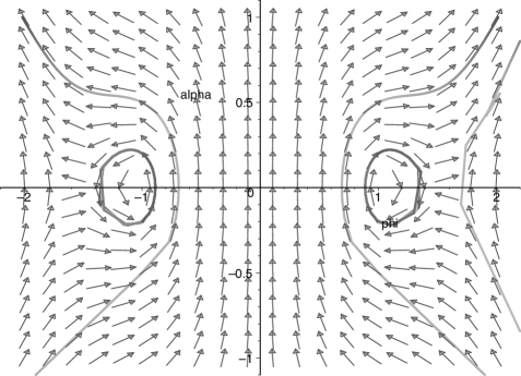
Figure 1: Field plot of the system of planar equations (38,39) coming from the wave function (37).For numerical simplicity we choose the values $-d=\sigma=1$. We see the two possibilities: trajectories corresponding to oscillating universes without singularities and trajectories corresponding to non-oscillating universes that come from a singularity, experience quantum effects in the middle of their expansions, and recover their classical behaviours for large values of $\alpha$.

IV The accelerated expansion.

IV.1 Qualitative approach

In this subsection we show how our approach for the explanation of the accelerated expansion works in a qualitative manner, i.e., with the parameters of the wave packet ($d$ and $\sigma$) adapted for readable numerical treatment, without any fitting with usual cosmological orders of magnitude. The aim is just to show that in some period in the history of such quantum models where the expansion is positively accelerated. We take here $d=-1$, $\sigma=1$ for the numerical computations. The quantum effects appearing in the middle of the non periodic bohmian trajectories described above can deviate them from their classical decelerated expansion to an accelerated one. We will show that this is indeed the case of this model. From $\alpha=\ln{a(t)}$ we have

$$\frac{\ddot{a}}{a}=\ddot{\alpha}+(\dot{\alpha})^{2}.$$ (40)

From Eq. (38), $\dot{\alpha}$ can be viewed as a function of the canonical variables $\dot{\alpha}=f(\alpha,\phi)$. Then we have

$$\ddot{\alpha}=\frac{\partial f}{\partial\alpha}\dot{\alpha}+\frac{\partial f}{\partial\phi}\dot{\phi}$$ (41)

Computing the derivatives with respect to $\alpha$ and $\phi$, and substituting $\dot{\alpha}$ and $\dot{\phi}$ from equations (38) and (39), respectively, we obtain

$$\frac{\ddot{a}}{a}=-\frac{1}{4}\biggr{[}\left(2{\phi}^{2}{\sigma}^{4}+\alpha{\sigma}^{4}\right)\left(\left(\sin(2d\phi)\right)^{2}\cos(2d\phi)+\left(\sin(2d\phi)\right)^{2}\cosh({\sigma}^{2}\alpha\phi)\right)+$$

$$\left(2{\sigma}^{2}d-2{\sigma}^{4}d{\phi}^{2}\right)\left(\sin(2d\phi)\cos(2d\phi)\sinh({\sigma}^{2}\alpha\phi)+\sin(2d\phi)\sinh({\sigma}^{2}\alpha\phi)\cosh({\sigma}^{2}\alpha\phi)\right)+$$

$$\left({\sigma}^{6}{\phi}^{3}+4{\sigma}^{2}{d}^{2}\phi-{\sigma}^{6}\phi{\alpha}^{2}\right)\left(\sin(2d\phi)\right)^{2}\sinh({\sigma}^{2}\alpha\phi)+\left(2{\sigma}^{4}d\phi\alpha-8{\sigma}^{2}d\phi\right)\sin(2d\phi)\left(\cos(2d\phi)\right)^{2}+$$

$$\left(2{\sigma}^{4}d\phi\alpha-16{\sigma}^{2}d\phi\right)\sin(2d\phi)\cos(2d\phi)\cosh({\sigma}^{2}\alpha\phi)+24{d}^{2}\left(\cos(2d\phi)\right)^{2}\cosh({\sigma}^{2}\alpha\phi)+$$

$$24{d}^{2}\cos(2d\phi)\left(\cosh({\sigma}^{2}\alpha\phi)\right)^{2}-8\phi d{\sigma}^{2}\sin(2d\phi)\left(\cosh({\sigma}^{2}\alpha\phi)\right)^{2}+4{\sigma}^{2}\phi{d}^{2}\left(\cos(2d\phi)\right)^{2}\sinh({\sigma}^{2}\alpha\phi)+$$

$$4{\sigma}^{2}\phi{d}^{2}\cos(2d\phi)\cosh({\sigma}^{2}\alpha\phi)\sinh({\sigma}^{2}\alpha\phi)+2{\sigma}^{4}\phi\left(\sin(2d\phi)\right)^{3}d\alpha-2{\sigma}^{4}\phi\sin(2d\phi)\left(\sinh({\sigma}^{2}\alpha\phi)\right)^{2}\alpha d+$$

$$8{d}^{2}\left(\cos(2d\phi)\right)^{3}+8{d}^{2}\left(\cosh({\sigma}^{2}\alpha\phi)\right)^{3}\biggl{]}\biggr{[}\left(e^{3\alpha}\right)^{2}\left(\cos(2d\phi)+\cosh({\sigma}^{2}\alpha\phi)\right)^{3}\biggl{]}^{-1}.$$ (42)

The equation above gives the acceleration $\frac{\ddot{a}}{a}$ as a function of $\alpha$ and $\phi$. If one integrates the system (38,39) to obtain $\phi=\phi(a)$, the quantum version of the classical equation (i.e. Raychaudhuri equation for the Friedmann model)

$$\frac{\ddot{a}}{a}=-\frac{4\pi G}{3}(\rho+3p)\propto-(\dot{\phi})^{2}\propto-\frac{1}{a^{6}}$$ (43)

can be obtained. Taking the limit where the absolute value of $\alpha$ is very large in Eq. (IV.1), one recovers the classical behaviour given in Eq. (43), $\frac{\ddot{a}}{a}\propto-1/a^{6}$. Note that the quantum analog of the Friedmann’s equation can also be easily obtained from Eqs.(30,31,32), yielding (recovering the unities) $H^{2}={\dot{\phi}}^{2}+\beta^{4}c^{2}Q(a,\phi)/a_{\rm phys}^{6}$.

We can represent $\frac{\ddot{a}}{a}$ in a tridimensional plot as a function of $\alpha$ and $\phi$. In this plot we can see the regions on the plane $\alpha-\phi$ in which the acceleration is possitive, negative or zero. We show this plot, for the parameters $d=-1$ and $\sigma=1$, in Fig. 2. One can see the classical behaviour $\ddot{a}/a\propto-1/a^{6}$ for $a\rightarrow 0$ ($\alpha\rightarrow-\infty$) and $a\rightarrow\infty$ ($\alpha\rightarrow\infty$), but near the region $a=1$ ($\alpha=0$), a clear departure from classical behaviour is observed, and positive values of $\ddot{a}/a$ are obtained. Fig. 3 shows the acceleration $\ddot{a}/a$ as a function of $\alpha$ for $\phi=1.66$.

As we pointed above, the quantum potential is the cause of this positive acceleration. Fig. 4 shows the quantum potential in the $\alpha-\phi$ plane where we can see that it is different from zero in the regions of positive acceleration. A trajectory passing through this region on the plane $\alpha-\phi$ will correspond to a universe experiencing an accelerated expansion. Fig. 5 shows the quantum potential as a function of $\alpha$ for $\phi=1.66$. Note also the increasing in the acceleration and in the quantum potential as we approach the node point $\alpha=0$, $\phi=\pi/2$.

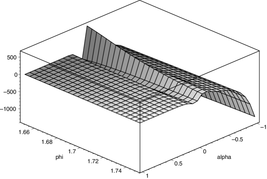
Figure 2: Acceleration $\ddot{a}/a$ as a function of $\phi$ and $\alpha$. For numerical simplicity we choose the values $-d=\sigma=1$.

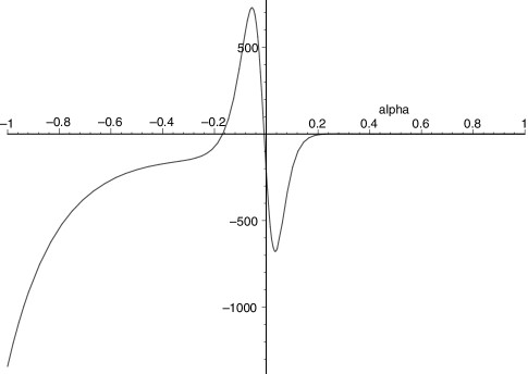
Figure 3: Acceleration $\ddot{a}/a$ as a function of $\alpha$ for $\phi=1.66$. For numerical simplicity we choose the values $-d=\sigma=1$.

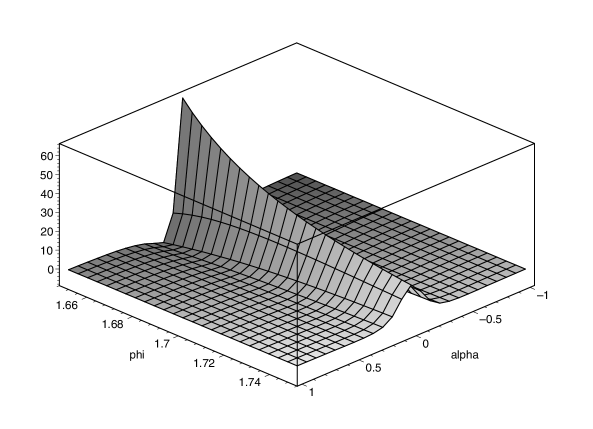
Figure 4: The quantum potential as a function of $\phi$ and $\alpha$. We see that it is different from zero in the region of positive acceleration. For numerical simplicity we choose the values $-d=\sigma=1$.

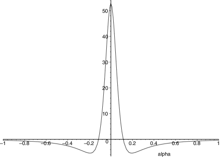
Figure 5: The quantum potential as a function of $\alpha$ for $\phi=1.66$. We see that it is different from zero in the region of positive acceleration. For numerical simplicity we choose the values $-d=\sigma=1$.

IV.2 Comparison between the quantum acceleration of the Universe’s expansion and the presence of a cosmological constant

We will now compare quantitatively the accelerated expansion of the Universe caused by such a quantum cosmological effect with the one generated by the presence of a cosmological constant in the classical model . First of all, we must recover the units in Eqs.(38,39). This is done by multiplying the RHS of these equations by $c/\beta$, where $\beta=\sqrt{\frac{4\pi}{3V}}l_{P}$ and $V=V_{{\rm phys}}(t)/a^{3}_{{\rm phys}}(t)$, where $a_{{\rm phys}}=a\beta$ is the physical scale factor and $V_{{\rm phys}}$ is the physical volume of the spacelike section. Then we obtain

$$H=\dot{\alpha}=f(\alpha,\phi)\frac{V_{P}}{V_{{\rm phys}}(t)t_{P}},$$ (44)

$$\dot{\phi}=g(\alpha,\phi)\frac{V_{P}}{V_{{\rm phys}}(t)t_{P}},$$ (45)

where

$$f(\alpha,\phi)=\frac{\phi\sigma^{2}\sin(2d\phi)}{2[\cos(2d\phi)+\cosh(\sigma^{2}\alpha\phi)]}-d,$$ (46)

$$g(\alpha,\phi)=-\frac{\alpha\sigma^{2}\sin(2d\phi)+2d\sinh(\sigma^{2}\alpha\phi)}{2[\cos(2d\phi)+\cosh(\sigma^{2}\alpha\phi)]},$$ (47)

$V_{P}\equiv\frac{4\pi}{3}l^{3}_{P}$ is the Planck volume, and $t_{P}$ is the Planck time. We will compare this quantum cosmological model with the original classical free scalar field model, classically equivalent to stiff matter, with flat spatial section, suplemented with a cosmological constant as an alternative source for accelerated expansion. This classical model satisfies the Friedmann s equation

$$H^{2}=\frac{8\pi G}{3}\frac{c_{\phi}}{a^{6}}+\Lambda=H_{0}^{2}[(1-\Omega_{\Lambda})(1+z)^{6}+\Omega_{\Lambda}],$$ (48)

where $c_{\phi}$ is a constant such that the energy density of the field is $\rho_{\phi}=c_{\phi}/a^{6}$, $\Omega_{\Lambda}=\Lambda/(8\pi G\rho_{\rm crit})$, $\rho_{\rm crit}$ is the critical density, and $H_{0}$ is the Hubble’s paremeter today. The deceleration parameter today, $q_{0}=-\ddot{a}/(a{H_{0}^{2}})$, is given by

$$q_{0}=2-3\Omega_{\Lambda}.$$ (49)

To obtain the luminosity distance as a function of $z$ one can calculate numerically the integral

$$d_{L}=(1+z)\int_{0}^{z}\frac{{\rm d}y}{H(y)}=\frac{(1+z)}{H_{0}}\int_{0}^{z}\frac{{\rm d}y}{\sqrt{(1-\Omega_{\Lambda})(1+y)^{6}+\Omega_{\Lambda}}}.$$ (50)

As a power series, it can be written as

$$H_{0}d_{L}=z+z^{2}\biggl{(}-\frac{1}{2}+\frac{3}{2}\Omega_{\Lambda}\biggr{)}+z^{3}(1-\Omega_{\Lambda})\biggl{(}\frac{1}{2}-\frac{9}{2}\Omega_{\Lambda}\biggr{)}+...,$$ (51)

In the quantum cosmological problem, we have to deal with Eqs. (44,45). There are four arbitrary parameters: $\sigma,d$ and two coordinates in the $(\alpha,\phi)$ plane, $\phi_{0}$ designating the particular trajectory in Fig.(1) which represent our Universe, and $\alpha_{0}$ designating the present moment in a particular trajectory. The present value of the Hubble’s paremeter in a particular trajectory coming from Eq.(44) is given by

$$H_{0}=f(\alpha_{0},\phi_{0})\frac{V_{P}}{V_{{\rm phys}}^{0}t_{P}}$$ (52)

where

$$f(\alpha_{0},\phi_{0})\equiv\frac{\phi_{0}\sigma^{2}\sin(2d\phi_{0})}{2[\cos(2d\phi_{0})+\cosh(\sigma^{2}\alpha_{0}\phi_{0})]}-d$$ (53)

In order to obtain a model similar to our present Universe whith $H_{0}\simeq 10^{-18}{\rm s}^{-1}$ and $V_{{\rm phys}}^{0}\geq 10^{82}{\rm cm}^{3}$, one must have

$$f(\alpha_{0},\phi_{0})\equiv\frac{\phi_{0}\sigma^{2}\sin(2d\phi_{0})}{2(\cos(2d\phi_{0})+\cosh(\sigma^{2}\alpha_{0}\phi_{0}))}-d\simeq 10^{120}$$ (54)

This huge number can be obtained by choosing a very large value for $\sigma^{2}$ (the gaussian in the wave function would be almost flat indicating no preference in the choice of $k$, or physically, no prefered choice in the strength of the initial explosion), a very large value for $|d|$ (a gaussian centered in a very negative value of $k$, or a choice for a very strong initial explosion), or trajectories passing very close to the node point, where the denominator of the above expression approaches zero.

In the case of a large value of $\sigma^{2}$, choosing $\alpha_{0}\simeq 1/\sigma^{4}\simeq 0$, one can check from Eq.(IV.1) that

$$q_{0}=-\frac{\ddot{a}}{a}|_{0}\frac{1}{H_{0}^{2}}\simeq\frac{2\cos(2d\phi_{0})+1}{\cos(2d\phi_{0})+1}$$ (55)

. For $2d\phi_{0}=2n\pi+x$ with $x\in(2.145,2.15)$ one has $-0.21<q_{0}<-0.17$. Note that, for the classical model with $\Omega_{\Lambda}=0.73$ new , $q_{0}=-0.19$ (see Eq. (49)).

The supernovae measurements relate the luminosity distance $d_{L}$ with $z$. Hence, it would be instructive to compare the quantum cosmological luminosity distance $d_{L}^{q}(z)$

$$d_{L}^{q}=(1+z)\int_{0}^{z}\frac{{\rm d}ye^{3\alpha(y)}}{f(\alpha(y),\phi(y))}\frac{\beta}{c},$$ (56)

with the one given in Eqs.(50,51). We will expande $G(y)\equiv e^{3\alpha(y)}/f(\alpha(y),\phi(y))$ in powers of $y$ around $y=0$ (today)

$$G(y)=G(0)+y\frac{{\rm d}G}{{\rm d}y}|_{y=0}+\frac{y^{2}}{2!}\frac{{\rm d}^{2}G}{{\rm d}y^{2}}|_{y=0}+\frac{y^{3}}{3!}\frac{{\rm d}^{3}G}{{\rm d}y^{3}}|_{y=0}+...$$ (57)

up to third order. The operator ${\rm d}/{\rm d}y$ can be written as

$$\frac{{\rm d}}{{\rm d}y}=-\frac{1}{(1+y)}\frac{{\rm d}}{{\rm d}\alpha}=-\frac{1}{(1+y)}\biggl{(}\frac{\partial}{\partial\alpha}+\frac{{\rm d}\phi}{{\rm d}\alpha}\frac{\partial}{\partial\phi}\biggr{)},$$ (58)

where ${\rm d}\phi/{\rm d}\alpha$ can be easily obtained from Eqs.(38,39) and $\alpha=\ln(a)=-\ln(1+y)+{\rm const.}$. Recalling that

$$\frac{H_{0}\beta a_{0}^{3}}{c}=\frac{H_{0}a_{\rm phys}^{3}}{c\beta^{2}}=\frac{H_{0}a_{\rm phys}^{3}l_{P}3V}{4\pi}=\frac{H_{0}t_{P}V_{\rm phys}}{V_{P}}\simeq 10^{120},$$ (59)

we obtain

$$H_{0}d_{L}^{q} = \frac{10^{120}}{f_{0}}\biggl{[}z+z^{2}\biggl{(}1+\frac{f_{0}}{2a_{0}^{3}}\frac{{\rm d}G}{{\rm d}z}|_{0}\biggr{)}+z^{3}\biggl{(}\frac{f_{0}}{2a_{0}^{3}}\frac{{\rm d}G}{{\rm d}z}|_{0}+\frac{f_{0}}{6a_{0}^{3}}\frac{{\rm d}^{2}G}{{\rm d}z^{2}}|_{0}\biggr{)}+$$ (60)

$$+z^{4}\biggl{(}\frac{f_{0}}{6a_{0}^{3}}\frac{{\rm d}^{2}G}{{\rm d}z^{2}}|_{0}+\frac{f_{0}}{24a_{0}^{3}}\frac{{\rm d}^{3}G}{{\rm d}z^{3}}|_{0}\biggr{)}+...\biggr{]}.$$

Comparing Eq.(60) with Eq.(51), one can see that $f_{0}$ must be of order $10^{120}$, as we have already concluded in Eq. (53). Here we will choose $|d|$ as the big number to make $f_{0}\simeq 10^{120}$, and $|\alpha_{0}|=\gamma/|d|$, $\gamma$ being an arbitrary number of order $1$. This is to assure that $\frac{{\rm d}^{n}G}{{\rm d}z^{n}}|_{0}$ is of order $1$ or less for any $n\geq 1$, which is not the case if we choose $\sigma\gg 1$. Using Eq.(58), we can calculate the coefficients in Eq.(60), obtaining

$$H_{0}d_{L}^{q} \simeq z-\frac{1}{2}z^{2}+z^{3}\biggl{\{}\frac{1}{2}+\frac{\phi_{0}^{2}\sigma^{4}}{6[1+\cos(2d\phi_{0})]^{2}}\biggr{\}}+$$ (61)

$$+z^{4}\biggl{\{}-\frac{1}{2}-\frac{\phi_{0}^{2}\sigma^{4}}{3[1+\cos(2d\phi_{0})]^{2}}-\frac{\phi_{0}^{3}\sigma^{6}\gamma\sin(2d\phi_{0})}{2[1+\cos(2d\phi_{0})]^{4}}\biggr{\}}+...$$

In order to obtain Eq.(61), we have used that $|d|>>1$ and $|\alpha_{0}|=\gamma/|d|$ is very small.

There are many values of $\phi_{0},\sigma_{0}$ and $\gamma$ which makes the graphic of $H_{0}d_{L}^{q}$ similar to the one obtained from Eq. (50) for $\Omega_{\Lambda}=0.73$. For instance, for $\gamma=1$ we set $2d\phi=0.64\pm 2n\pi$ and the coefficients of $z^{3}$ and $z^{4}$ become, respectively, $2.6$ and $-2.25$.

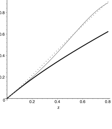
Figure 6: The luminosity distance as a function of redshift. The thin line curve corresponds to the quantum model, the dotted curve is for the classical model with a cosmological constant, and the thick line curve is for the classical model without cosmological constant.

In Fig.6, we show a plot of $H_{0}d_{L}(z)$ given by Eq.(50), $H_{0}d_{L}(z)$ given by Eq.(50) with $\Omega_{Lambda}=0$, and $H_{0}d_{L}^{q}(z)$ given by Eq.(61) with the coefficients of $z^{3}$ and $z^{4}$ being equal to $2.6$ and $-2.25$, respectively. Note that for small values of $z$ they are close but, for intermediary values of $z$, the quantum $d_{L}^{q}(z)$ remain close to the cosmological constant $d_{L}(z)$ while both separates of the pure stiff matter $d_{L}(z)$. Of course, for bigger values of $z$, the quantum $d_{L}^{q}(z)$ may separate strongly from the cosmological constant $d_{L}(z)$. Hence, quantum comological effects may mimic a cosmological constant in some region but not everywhere. The two models are distinguishable.

V Conclusion

We have studied gaussian superpositions of positive and negative frequency mode solutions of the Wheeler-DeWitt equation corresponding to a scalar-tensor model in minisuperspace in the case of flat spatial section. According to the Bohm-de Broglie approach to quantum cosmology, the quantum trajectories representing dynamical universes evolving in time were studied. We have shown that it is possible to have universes which arise classically from a singularity, undergo a positive acceleration in the middle of its expansion, and recover its classical behaviour for large values of the scale factor. We have shown that this positive acceleration, which can be made compatible with observations for many choices of initial conditions, is due to a quantum cosmological effect driven by the quantum potential, according to the BdB interpretation of quantum cosmology. In this way, it may be possible to explain the positive acceleration suggested by the recent measurements of high redshift supernovae without postulating a new contribution to the energy density of the Universe as the dark energy. Note that this acceleration is caused by quantum effects not only present in the scalar field, as described in Ref.parker , but also in the geometry itself. We consider the Universe as a quantum system no matter its size. It is possible to have small classical universes and large quantum ones: it depends on the state functional and on initial conditions fab ; hartle .

The quantum cosmological explanation for the acceleration of the Universe presented in this paper needs to be studied further, not only because it would be an alternative explanation for a misterious behaviour of the present Universe without appealing to any new form of energy, but also because it is a possibility of an observable physical effect of quantum cosmology. Furthermore, quantum cosmological explanations may be suported by symmetry principles which are absent in the classical domain. As an example, we have seen that the huge cosmological numbers may be explained by some ”democracy” principle stating that any value of the velocity of expansion (the constant $k$) is equally good ($\sigma$ is very big, the gaussian is almost flat). Of course, more elaborated models taking into account relevant matter sources like dust and radiation must be studied. This will be the subject of our future investigations.

References

- (1) R. Colistete Jr., J. C. Fabris and N. Pinto-Neto, Phys. Rev. D62, 83507 (2000).
- (2) S. Perlmutter, et al., Nature (London) 391, 51 (1998).
- (3) A. Riess et al., Astron. J. 116, 1009, (1998).
- (4) Neta A. Bahcall, J. P. Ostriker, S. Perlmutter and P. J. Steinhardt, Science 284, 1481-1488 (1999).
- (5) P.M. Garnavich et al., Astrophys.J. 509,74 (1998).
- (6) L. Wang, R.R. Caldwell, J.P. Ostriker and Paul J. Steinhardt Astrophys. J. 530, 17-35 (2000).
- (7) R. R. Caldwell, R. Dave and P. J. Steinhardt, Phys. Rev. Lett.80, 1582 (1998);
- (8) Philippe Brax and Jerome Martin, Phys.Rev. D61 103502 (2000).
- (9) R. Colistete Jr., J. C. Fabris and N. Pinto-Neto, Phys. Rev. D57, 4707 (1998).
- (10) David Bohm, Phys. Rev. 85, 166 (1952).
- (11) David Bohm, Phys. Rev. 85, 180 (1952).
- (12) P. R. Holland, The Quantum Theory of Motion: An Account of the de Broglie-Bohm Causal Interpretation of Quantum Mechanics (Cambridge University Press, Cambridge, 1993).
- (13) B. S. DeWitt and N. Graham (Eds.) The Many-Worlds Interpretation of Quantum Mechanics (Princeton University Press, Princeton, 1973).
- (14) Jonathan J. Halliwell and James B. Hartle, Phys. Rev. D 41, 1815 (1990).
- (15) Leonard Parker and Alpan Raval, Phys. Rev. Lett. 86, 749 (2001).
- (16) V. A. De Lorenci, J. Martin, N. Pinto-Neto and I. Damião Soares, Phys.Rev. D 56, 3329 (1997).
- (17) P. A. M. Dirac, Lectures on Quantum Mechanics, Yeshiva University (1964).
- (18) J. Acácio de Barros and N. Pinto-Neto, Int. J. of Mod. Phys. D 7, 201 (1998).
- (19) N. Pinto-Neto and E. Sergio Santini, Phys.Rev. D 59 123517 (1999).
- (20) N. Pinto-Neto and E. Sergio Santini, Gen. Rel. and Grav. 34, 505 (2002).
- (21) E. Sergio Santini, PhD Thesis, CBPF-Rio de Janeiro, (May 2000), (gr-qc/0005092).
- (22) C. L. Bennett et al., astro-ph/0302207.