Close encounters of black holes

Abstract

This is an introduction into the problem of how to set up black hole initial-data for the matter-free field equations of General Relativity. The approach is semi-pedagogical and addresses a more general audience of astrophysicists and students with no specialized training in General Relativity beyond that of an introductory lecture.

1 Introduction and motivation

In my lecture I will try to explain how scattering and merging processes between black holes can be described analytically in general relativity(GR). This is a vast subject and I will focus attention to the basic issues, rather than trying to explain analytical details of approximation schemes etc. I will also not discuss numerical aspects, which are beyond my competence, and which would anyway require a separate lecture. I will address the following main topics:

1. a first step beyond Newtonian gravity,

2. constrained evolutionary structure of Einstein’s equations,

3. the 3+1- split and the Cauchy initial-value problem,

4. black hole data,

5. problems and recent developments,

with emphasis on the fourth entry. However, I will also spend some time to explain some of the specialties of GR, like the absence of a point-particle concept and the non-trivial linkage between the field equations and the equations of motion for matter. These points should definitely be appreciated before one goes on to discuss black holes, which are solutions to the vacuum Einstein equations representing extended objects.

The following points seem to me the main motivations for studying the problem of black hole collision:

• Coalescing black holes are regarded as promising sources for the detection of gravitational waves by earth-based instruments.

• Close encounters of black holes provide physically relevant situations for the investigation of the strong-field regime of general relativity.

• The dynamics of simple black hole configurations is regarded as ideal testbed for numerical relativity.

My conventions are as follows: space-time is a manifold $M$ with Lorentzian metric $g$ of signature $(-,+,+,+)$. Greek indices range from $0$ to $3$, latin indices from $1$ to $3$ unless stated otherwise. The covariant derivative is denoted $\nabla_{\mu}$, ordinary partial derivatives by $\partial_{\mu}$ or sometimes simply by a lower-case $,\mu$. The relation $:=$ ($=:$) defines the left (right) hand side. The gravitational constant in GR is $\kappa=8\pi G/c^{2}$, where $G$ is Newton’s constant and $c$ the velocity of light. A symbol like $O(\epsilon^{n})$ stands collectively for terms falling off at least as fast as $\epsilon^{n}$.

2 A first step beyond Newtonian gravity

It can hardly be overstressed how useful the concept of a mass-point is in Newtonian mechanics and gravity. It allows to pointwise probe the gravitational field and to reduce the dynamical problem to the mathematical problem of finding solutions to a system of finitely many ordinary differential equations. To be sure, just postulating the existence of mass points is not sufficient. To be consistent with known laws of physics one must eventually understand the point mass as an idealization of a highly localized mass distribution which obeys known field-theoretic laws, such that in the situations at hand most of the field degrees of freedom effectively decouple from the dynamical laws for those collective degrees of freedom one is interested in, like e.g. the centre-of-mass. In Newtonian gravity this usually requires clever approximation schemes but is not considered to be a problem of fundamental nature. Although this is true for the specific linear theory of Newtonian gravity, this needs not be so for comparably simple generalizations, as will become clear below.

In GR the situation is markedly different. A concentration of more than one Schwarzschild mass in a region of radius less than the Schwarzschild radius will lead to a black hole whose behaviour away from the stationary state usually cannot be well described by finitely many degrees of freedom. It shakes and vibrates, thereby radiating off energy and angular momentum in form of gravitational radiation. Moreover, it is an extended object and cannot be unambiguously ascribed an (absolute or relative) position or individual mass. Hence the problem of motion, and therefore the problem of scattering of black holes, cannot be expected to merely consist of corrections to Newtonian scattering problems. Rather, the whole kinematic and dynamical setup will be different where many of the established concepts of Newtonian physics need to be replaced or at least adapted, very often in a somewhat ambiguous way. Among those are mass, distance, and kinetic energy. For example, one may try to solve the following straightforward sounding problem in GR, whose solution one might think has been given long ago. Given are two unspinning black holes, momentarily at rest, with equal individual mass $m$, mutual distance $\ell$, and no initial gravitational radiation around. What is the amount of energy released via gravitational radiation during the dynamical infall? In such situation we can usually make sense of the notions of ‘spin’ (hence unspinning) and ‘mass’; but ambiguities generally exist in defining ‘distance’ and, most important of all, ‘initial gravitational radiation’. Such difficulties persist over and above the ubiquitous analytical and/or numerical problems which are currently under attack by many research groups.

To those who are not so familiar with GR and like to see Newtonian analogies, I wish to mention that there is a way to consistently model some of the non-linear features of Einstein’s equations in a Newtonian context, which shares the property that it does not allow for point masses. I will briefly describe this model since it does not seem to be widely known.

First recall the field equation in Newtonian gravity, which allows to determine the gravitational potential $\phi$ (whose negative gradient, -$\vec{\nabla}\phi$, is the gravitational field) from the mass density $\rho$ (the ‘source’ of the gravitational field):

$$\Delta\phi=4\pi G\rho\,.$$ (1)

Now suppose one imposes the following principle for a modification of (1): all energies, including the self-energy of the gravitational field, act as source for the gravitational field. In order to convert an energy density $\varepsilon$ into a mass density $\rho$, we adopt the relation $\varepsilon=\rho c^{2}$ from special relativity (the equation we will arrive at can easily be made Lorentz invariant by adding appropriate time-derivatives). The question then is whether one can modify the source term of (1) such that $\rho\rightarrow\rho+\rho_{\scriptscriptstyle\rm grav}$ with $\rho_{\scriptscriptstyle\rm grav}:=\varepsilon_{\scriptscriptstyle\rm grav}/c^{2}$, where $\varepsilon_{\scriptscriptstyle\rm grav}$ is the energy density of the gravitational field as predicted by this very same equation (condition of self-consistency). It turns out that there is indeed a unique such modification, which reads

$$\Delta\phi=\frac{4\pi G}{c^{2}}\,\phi\left[\rho+\frac{c^{2}}{8\pi G}(\vec{\nabla}\phi/\phi)^{2}\right]\,.$$ (2)

It is shown in the Appendix that this equation indeed satisfies the ‘energy principle’ as just stated. (For more information and a proof of uniqueness, see [21].) The gravitational potential is now required to be always positive, tending to the value $c^{2}$ at spatial infinity (rather than zero as for (1)). The second term on the right hand side of (2) corresponds to the energy density of the gravitational field. Unlike the energy density following from (1) (which is $-\frac{1}{8\pi G}|\nabla\phi|^{2}$) it is now positive definite. This does not contradict attractivity of gravity for the following reason: the rest-energy density of a piece of matter is in this theory not given by $\rho c^{2}$, but by $\rho\phi$, that is, it depends on the value of the gravitational potential at the location of matter. The same piece of matter located at lower gravitational potential has less energy than at higher potential values. In GR this is called the universal redshift effect. Here, as in GR, the active gravitational-mass also suffers from this redshift, as is immediate from the first term on the right hand side of (2), where $\rho$ does not enter alone, as in (1), but is multiplied with the gravitational potential $\phi$. With respect to these features our modification (2) of Newtonian gravity mimics GR quite well.

We mention in passing that (2) can be ‘linearized’ by introducing the dimensionless field $\psi:=\sqrt{\phi}/c$, in terms of which (2) reads

$$\Delta\psi=\frac{2\pi G}{c^{2}}\rho\psi\,.$$ (3)

The boundary conditions are now $\psi(r\rightarrow\infty)\rightarrow 1$. Hence only those linear combinations of solutions are again solutions whose coefficients add up to one. For $\rho\geq 0$ it also follows that solutions to (3) can never assume negative values, since otherwise the function $\psi$ must have a negative minimum (because of the positive boundary values) and therefore non-negative second derivatives there. But then (3) cannot be satisfied at the minimum, hence $\psi$ must be nonnegative everywhere. This implies that solutions of (2) are also non-negative. To be sure, for mathematical purposes (3) is easier to use than (2), but note that $\phi$ and not $\psi$ is the physical gravitational potential.

We now show how these non-linear features render impossible the notion of point mass, and even induce a certain black-hole behaviour on their solutions. Let us be interested in static, spherically symmetric solutions to (2) with source $\rho$, which is zero for $r>R$ and constant for $r<R$. We need to distinguish two notions of mass. One mass just counts the amount of ‘stuff’ located within $r<R$. You may call it ‘bare mass’ or ‘baryonic mass’, since for ordinary matter it is proportional to the baryon number. We denote it by $M_{B}$. It is simply given by

$$M_{B}:=\int_{\rm\scriptscriptstyle space}d^{3}x\ \rho\,.$$ (4)

The other mass is the ‘gravitational mass’, which is measured by the amount of flux of the gravitational field to ‘infinity’, that is, through the surface of a sphere whose radius tends to infinity. We call this mass $M_{G}$. It is given by

$$M_{G}:=\frac{1}{4\pi G}\lim_{r\rightarrow\infty}\int_{S^{2}(r)}(-\vec{\nabla}\phi\cdot\vec{n})\,d\sigma\,,$$ (5)

where $r=|\vec{x}|$, $\vec{x}/r=\vec{n}$, $S^{2}(r)$ is the 2-sphere or radius $r$ and $d\sigma$ is its surface element. $M_{G}$ should be identified with the total inertial mass of the system, in full analogy to the ADM-mass in GR (see eq. (35) below). Hence $M_{G}c^{2}$ is the total energy of the system, with gravitational binding energy also taken into account. The masses $M_{B}$ and $M_{G}$ can dimensionally be turned into radii by writing $R_{B}:=GM_{B}/c^{2}$ and $R_{G}:=GM_{G}/c^{2}$, and further turned into dimensionless quantities via rescaling with $R$, the radius of our homogeneous star. We write $x:=R_{B}/R$ and $y:=R_{G}/R$.

For each pair of values for the two parameters $M_{B}$ and $R$ there is a unique homogeneous-star-solution to (2), whose simple analytical form needs not interest us here (see [21]). Using it we can calculate $M_{G}$, whose dependence on the parameters is best expressed in terms of the dimensionless quantities $x$ and $y$:

$$y=f(x)=2\,\left(1-\frac{\tanh(\sqrt{3x/2})}{\sqrt{3x/2}}\right)\,.$$ (6)

The function $f$ maps the interval $[0,\infty]$ monotonically to $[0,2]$. This implies the following inequality

$$M_{G}<2Rc^{2}/G$$ (7)

which says that the gravitational mass of the star is bounded by a purely geometric quantity. It corresponds to the statement in GR that the star’s radius must be bigger than its Schwarzschild radius, which in isotropic coordinates is indeed given by $R_{S}=GM_{G}/2c^{2}$. It can be proven [21] that the bound (7) still exists for non-homogeneous spherically symmetric stars, so that the somewhat unphysical homogeneity assumption can be lifted. The physical reason for this inequality is the ‘redshift’, i.e. the fact, that the same bare mass at lower gravitational potential produces less gravitational mass. Hence adding more and more bare mass into the same volume pushes the potential closer and closer to zero (recall that $\phi$ is always positive) so that the added mass becomes less and less effective in generating gravitational fields. The inequality then expresses the mathematical fact that this ‘redshifting’ is sufficiently effective so as to give finite upper bounds to the gravitational mass, even for unbounded amounts of bare mass.

The energy balance can also be nicely exhibited. Integrating the matter energy density $\phi\rho$ and the energy density of the gravitational field, $\frac{c^{4}}{8\pi G}(\vec{\nabla}\phi/\phi)^{2}$, we obtain

$$E_{\rm\scriptscriptstyle matter} = M_{B}c^{2}\,\left(1-\frac{6R_{B}}{5R}+O(R_{B}^{2}/R^{2})\right)\,,$$ (8)

$$E_{\rm\scriptscriptstyle field} = M_{B}c^{2}\,\left(\frac{3R_{B}}{5R}+O(R_{B}^{2}/R^{2})\right)\,,$$ (9)

$$E_{\rm\scriptscriptstyle total} = M_{B}c^{2}\,\left(1-\frac{3R_{B}}{5R}+O(R_{B}^{2}/R^{2})\right)=M_{G}c^{2}\,.$$ (10)

Note that the term $-3M_{B}c^{2}R_{B}/5R$ in (10) is just the Newtonian binding energy. At this point it is instructive to verify the remarks we made above about the positivity of the gravitational energy. Shrinking a mass distribution enhances the field energy, but diminishes the matter energy twice as fast, so that the overall energy is also diminished, as it must due to the attractivity of gravity. But here this is achieved with all energies involved being positive, unlike in Newtonian gravity. Note that the total energy, $M_{G}$, cannot become negative (since $\phi$ cannot become negative, as already shown). Hence one also cannot extract an infinite amount of energy by unlimited compression, as it is possible in Newtonian gravity. This is the analogue in our model theory to the positive mass theorem in GR.

We conclude by making the point announced above, namely that the inequality (7) shows that point objects of finite gravitational mass do not exist in the theory based upon (2); mass implies extension! Taken together with the lesson from special relativity, that extended rigid bodies also do not exist (since the speed of elastic waves is less than $c$), we arrive at the conclusion that the dynamical problem of gravitating bodies and their interaction is fundamentally of field-theoretic (rather than point-mechanical) nature. Its proper realization is GR to which we now turn.

3 Constrained evolutionary structure of Einstein’s equations

In GR the basic field is the spacetime metric $g_{\mu\nu}$, which comprises the gravitational and inertial properties of spacetime. It defines what inertial motion is, namely a geodesic

$${\ddot{x}}^{\lambda}+\Gamma^{\lambda}_{\mu\nu}{\dot{x}}^{\mu}{\dot{x}}^{\nu}=0$$ (11)

with respect to the Levi-Civita connection

$$\Gamma^{\lambda}_{\mu\nu}:=\hbox{${\textstyle{\frac{1}{2}}}$}g^{\lambda\sigma}(-g_{\mu\nu,\sigma}+g_{\sigma\mu,\nu}+g_{\nu\sigma,\mu})\,.$$ (12)

(Since inertial motion is ‘force-free’ by definition, you may rightly ask whether it is correct to call gravity a ‘force’.) The gravitational field $g_{\mu\nu}$ is linked to the matter content of spacetime, represented in form of the energy momentum tensor $T_{\mu\nu}$, by Einstein’s equations

$$G_{\mu\nu}:=R_{\mu\nu}-\hbox{${\textstyle{\frac{1}{2}}}$}g_{\mu\nu}R=\kappa T_{\mu\nu}.$$ (13)

Due to the gauge-invariance with respect to general differentiable point transformations (i.e. diffeomorphisms) of spacetime one has the identities (as a consequence of Noether’s 2nd theorem)

$$\nabla_{\mu}G^{\mu\nu}\equiv 0\,.$$ (14)

Being ‘identities’ they hold for any $G^{\mu\nu}$, independent of any field equation. With respect to some coordinate system $x^{\mu}=(x^{0},\cdots x^{3})$ we can expand (14) in terms of ordinary derivatives. Preferring the coordinate $x^{0}$, this reads

$$\partial_{0}G^{0\nu}=-\partial_{k}G^{k\nu}-\Gamma^{\mu}_{\mu\lambda}G^{\lambda\nu}-\Gamma^{\nu}_{\mu\lambda}G^{\mu\lambda}.$$ (15)

Since $G^{\mu\nu}$ contains no higher derivatives of $g_{\mu\nu}$ than the second, the right-hand side of this equation also contains only 2nd $x^{0}$-derivatives. Hence (15) implies that the four components $G^{0\nu}$ only involve first $x^{0}$-derivatives. Now choose $x^{0}$ as time coordinate. The four $(0,\nu)$-components of (13) then do not involve second time derivatives, unlike the space-space components $(i,j)$. Hence the time-time and time-space components are constraints, that is, equations that constrain the allowed choices of initial data, rather than evolving them.

That is not an unfamiliar situation, which similarly occurs for Maxwell’s equations in electromagnetism (EM). Let us recall this analogy. We consider the four-dimensional form of Maxwell’s equations in terms of the vector potential $A_{\mu}$, whose antisymmetric derivative is the field-tensor $F_{\mu\nu}:=\partial_{\mu}A_{\nu}-\partial_{\nu}A_{\mu}$, comprising the electric ($E_{i}=F_{0i}$) and magnetic ($B_{i}=-F_{jk}$, $ijk$ cyclic) field. Maxwell’s equations are

$$E^{\nu}:=\partial_{\mu}F^{\mu\nu}-{\textstyle\frac{4\pi}{c}}j^{\nu}=0\,.$$ (16)

Due to its antisymmetry, the field tensor obviously obeys the identity

$$\partial_{\mu}\partial_{\nu}F^{\mu\nu}\equiv 0\,,$$ (17)

which here is the analogue of (14), an identity involving third derivatives in the field variables. Using (17) in the divergence of (16) yields

$$\partial_{\nu}E^{\nu}=-{\textstyle\frac{4\pi}{c}}\partial_{\nu}j^{\nu}\,,$$ (18)

which shows that Maxwell’s equations imply charge conservation as integrability condition. Let us interpret the rôle of charge conservation in the initial value problem. Decomposing (17) into space and time derivatives gives

$$\partial_{0}\partial_{\nu}F^{0\nu}=-\partial_{k}\partial_{\nu}F^{k\nu}\,.$$ (19)

Again the right hand side involves only second time derivatives implying that the $0$-component of (16) involves no second time derivatives. Hence the time component of (16) is merely a constraint on the initial data; clearly it is just Gauss’ law $\vec{\nabla}\cdot\vec{E}-4\pi\rho=0$. Its change under time evolution according to Maxwell’s equations is

$$\partial_{0}E^{0} = \partial_{\nu}E^{\nu}-\partial_{k}E^{k}$$ (20)

$$= -{\textstyle\frac{4\pi}{c}}\partial_{\nu}j^{\nu}-\partial_{k}E^{k}\,,$$

where we used the identity (18) in the second step. Suppose now that on the initial surface of constant $x^{0}$ we put an electromagnetic field which satisfies the constraint, $E^{0}=0$, and which we evolve according to $E^{k}=0$ (implying $\partial_{k}E^{k}=0$ on that initial surface). Then (20) shows that charge conservation is the necessary and sufficient condition for the evolution to preserve the constraint.

Let us return to GR now, where the overall situation is entirely analogous. Now we have four constraints

$$E^{0\nu}:=G^{0\nu}-\kappa T^{0\nu}=0$$ (21)

and six evolution equations, which we write

$$E^{ij}:=G^{ij}-\kappa T^{ij}=0\,.$$ (22)

The identity (14) now implies

$$\nabla_{\mu}E^{\mu\nu}=-\kappa\nabla_{\mu}T^{\mu\nu}\,,$$ (23)

which parallels (18). Here, too, the time derivative of the constraints is easily calculated:

$$\partial_{0}E^{0\nu} = \nabla_{\mu}E^{\mu\nu}-\partial_{k}E^{k\nu}-\Gamma^{0}_{0\lambda}E^{\lambda\nu}-\Gamma^{\nu}_{0\lambda}E^{0\lambda}$$ (24)

$$= -\kappa\nabla_{\mu}T^{\mu\nu}-\partial_{k}E^{k\nu}-\Gamma^{0}_{0\lambda}E^{\lambda\nu}-\Gamma^{\nu}_{0\lambda}E^{0\lambda}$$

using (23) in the last step. Now consider again the evolution of initial data from a surface of constant $x^{0}$. If they initially satisfy the constraints and are evolved via $E^{ij}=0$ (hence all spatial derivatives of $E^{\mu\nu}$ vanish initially) they continue to satisfy the constraints if and only if the energy momentum tensor of the matter satisfies

$$\nabla_{\mu}T^{\mu\nu}=0\,.$$ (25)

Hence we see that the ‘covariant conservation’ of energy-momentum, expressed by (25), plays the same rôle in GR as charge conservation plays in EM. This means that you cannot just prescribe the motion of matter and then use Einstein’s equations to calculate the gravitational field produced by that source. You have to move the matter in such a way that it satisfies (25). But note that at this point there is a crucial mathematical difference to charge conservation in EM: charge conservation is a condition on the source only, it does not involve the electromagnetic field. This means that you know a priori what to do in order not to violate charge conservation. On the other hand, (25) involves the source and the gravitational field. The latter enters through the covariant derivatives which involve the metric $g_{\mu\nu}$ through the connection coefficients (12). Hence here (25) cannot be solved a priori by suitably restricting the motion of the source. Rather we have a consistency condition which mutually links the problem of motion for the sources and the problem of field determination. It is this difference which makes the problem of motion in GR exceedingly difficult. (A brief and lucid presentation of this problem, drawing attention to its relevance in calculating the generation of gravitational radiation by self-gravitating systems, was given in [15]. A broader summary, including modern developments is [14]).

For example, for pressureless dust represented by $T^{\mu\nu}=\rho c^{2}\,U^{\mu}U^{\nu}$, where $\rho$ is the local rest-mass density and $U^{\mu}$ is the vector field of four-velocities of the continuously dispersed individual dust grains, (25) is equivalent to the two equations

$$\nabla_{\mu}(\rho U^{\mu}) = 0\,,$$ (26)

$$U^{\nu}\nabla_{\nu}U^{\mu} = 0\,.$$ (27)

The first states the conservation of rest-mass. The second is equivalent to the statement that the vector field $U^{\mu}$ is geodesic, which means that its integral lines (the worldlines of the dust grains) are geodesic curves (11) with respect to the metric $g_{\mu\nu}$. Hence we see that in this case the motion of matter is fully determined by (25), i.e. by Einstein’s equations, which imply (25) as integrability condition. This clearly demonstrates how the problem of motion is inseparably linked with the problem of field determination, and that these problems can only be solved simultaneously. The methods used today use clever approximation schemes. For example, one can make use of the fact that there is a difference of one power in $\kappa$ between the field equations and their integrability condition. Hence, in an approximation in $\kappa$ it is consistent for the $n$th order approximation of the field equations to have the integrability conditions (equations of motions) satisfied to $n-1$st order.

Clearly the problem just discussed does not arise for the matter-free Einstein equations for which $T_{\mu\nu}\equiv 0$. Now recall that black holes too are described by the matter free equations. Hence the mathematical problem just described does not occur in the discussion of their dynamics. In this aspect the discussion of black hole scattering is considerably easier than e.g. that of neutron stars.

4 The 3+1- split and the Cauchy initial-value problem

We saw that the ten Einstein equations decompose into two sets of four and six equations respectively, four constraints which the initial data have to satisfy, and six equations driving the evolution. As a consequence there will be four dynamically undetermined components among the ten components of the gravitational field $g_{\mu\nu}$. The task is to parametrise the $g_{\mu\nu}$ in such a way that four dynamically undetermined functions can be cleanly separated from the other six. One way to achieve this is via the splitting of spacetime into space and time (see [22] for a more detailed discussion). The four dynamically undetermined quantities will be the famous lapse (one function $\alpha$) and shift (three functions $\beta^{i}$). The dynamically determined quantity is the Riemannian metric $h_{ij}$ on the spatial 3-manifolds of constant time. These together parametrise $g_{\mu\nu}$ as follows:

$$ds^{2}=-\alpha^{2}\,(dx^{0})^{2}+h_{ik}\,(dx^{i}+\beta^{i}dx^{0})(dx^{k}+\beta^{k}dx^{0})\,.$$ (28)

The physical interpretation of $\alpha$ and $\beta^{i}$ is as follows: think of spacetime as the history of space. Each ‘moment’ of time, $x^{0}=t$, corresponds to an entire 3-dimensional slice $\Sigma_{t}$. Obviously there is plenty of freedom how to ‘waft’ space through spacetime. This freedom corresponds precisely to the freedom to choose the 1+3 functions $\alpha$ and $\beta^{i}$. For one thing, you may freely specify how far for each parameter step $dt$ you push space in a perpendicular direction forward in time. This is controlled by $\alpha$, which is just the ratio $ds/dt$ of the proper perpendicular distance between the hypersurfaces $\Sigma_{t}$ and $\Sigma_{t+dt}$. This speed may be chosen in a space and time dependent fashion, which makes $\alpha$ a function on spacetime. Second, given a point with coordinates $x^{i}$ on $\Sigma_{t}$. Going from $x^{i}$ in a perpendicular direction you meet $\Sigma_{t+dt}$ in a point with coordinates $x^{i}+dxi$, where $dx^{i}$ can be chosen at will. This freedom of moving the coordinate system around while evolving is captured by $\beta^{i}$; one writes $dx^{i}=\beta^{i}dt$. Clearly this moving around of the spatial coordinates can also be made in a space and time dependent fashion, so that the $\beta^{i}$ are functions of spacetime, too.

Let $n^{\mu}$ be the vector field in spacetime which is normal to the spatial sections of constant time. It is given by $n=\frac{1}{\alpha}(\partial/\partial x^{0}-\beta^{i}\partial/\partial x^{i})$, as one may readily verify using (28) (you have to check that $n$ is normalized and satisfies $g(n,\partial/\partial x^{i})=0$). We define the extrinsic curvature, $K_{ij}$, to be one-half the Lie derivative of the spatial metric in the direction of the normal:

$$K_{ij}:=\hbox{${\textstyle{\frac{1}{2}}}$}L_{n}h_{ij}=\frac{1}{2\alpha}\left(\frac{\partial h_{ij}}{\partial x^{0}}-2D_{(i}\beta_{j)}\right)\,,$$ (29)

where $D$ is the spatial covariant derivative with respect to the metric $h_{ij}$. As usual, a round bracket around indices denotes their symmetrization. Note that, by definition, $K_{ij}$ is symmetric. Finally we denote the Ricci scalar of $h_{ij}$ by $R^{\scriptscriptstyle(3)}$.

We can now write down the four constraints of the vacuum Einstein equations in terms of these variables:

$$0 = G(n,n)=\hbox{${\textstyle{\frac{1}{2}}}$}(R^{\scriptscriptstyle(3)}+K^{ij}K_{ij}-(K^{i}_{i})^{2})\,,$$ (30)

$$0 = G(n,\partial/\partial x^{j})=D_{i}(K^{i}_{j}-\delta^{i}_{j}K^{k}_{k})\,.$$ (31)

(30) and (31) are referred to as Hamiltonian constraint and momentum constraint respectively. The six evolution equations of second order in the time derivative can now be written as twelve equations of first order. Six of them are just (29), read as equation that relates the time derivative $\partial h_{ij}/\partial x^{0}$ to the ‘canonical data’ $(h_{ij},K_{ij})$. The other six equations, whose explicit form needs not concern us here (see e.g. [22]), express the time derivative of $K_{ij}$ in terms of the canonical data. Both sets of evolution equations contain on their right hand sides the lapse and shift functions, whose evolution is not determined but must be specified by hand. This specification is a choice of gauge, without which one cannot determine the evolution of the physical variables $(h_{ij},K_{ij})$.

The initial-data problem takes now the following form

1. Choose a topological 3-manifold $\Sigma$.

2. Find on $\Sigma$ a Riemannian metric $h_{ij}$ and a symmetric tensor field $K_{ij}$ which satisfy the constraints (30) and (31).

3. Choose a lapse function $\alpha$ and a shift vector field $\beta^{i}$, both as functions of space and time, possibly according to some convenient prescription (e.g. singularity avoiding gauges, like maximal slicing).

4. Evolve initial data with these choices of $\alpha$ and $\beta^{i}$ according to the twelve equations of first order. By consistency of Einstein’s equations the constraints will be preserved during this evolution, independent of the choices for $\alpha$ and $\beta^{i}$.

The backbone of this setup is a mathematical theorem, which states that for any set of initial data, taken from a suitable function space, there is, up to diffeomorphism, a unique maximal Einstein spacetime developing from these data [7].

5 Black hole data

5.1 Horizons

By black hole data we understand vacuum data which contain apparent horizons. The informal definition of an apparent horizon is that it is the boundary of a trapped region, which means that its orthogonal outgoing null rays must have zero divergence. (Inside the trapped region they converge for any 2-surface, by definition of ‘trapped region’.) The Penrose-Hawking singularity theorems state that the existence of an apparent horizon implies that the evolving spacetime will be singular (assuming the strong energy-condition). Given also the condition that singularities cannot be seen by observers far off, a condition usually called cosmic censorship, one infers the existence of an event horizon and hence a black hole. One can then show that the intersection of the event horizon with the spatial hypersurface lies on or outside the apparent horizon (for stationary spacetimes they coincide). The reason why one does not deal with event horizons directly is that you cannot tell whether there exists one by just looking at initial data. In principle you would have to evolve them to the infinite future, which is beyond our abilities in general. In contrast, apparent horizons can be recognized once the data on an initial slice are given. The formal definition of an apparent horizon is the following: given initial data $(\Sigma,h_{ij},K_{ij})$ and an embedded 2-surface $\sigma\subset\Sigma$ with outward pointing normal $\nu^{i}$. $\sigma$ is an apparent horizon if and only if the following relation between $K_{ij}$, the extrinsic curvature of $\Sigma$ in spacetime, and $k_{ij}$, the extrinsic curvature of $\sigma$ in $\Sigma$, is satisfied:

$$q^{ij}k_{ij}=-q^{ij}K_{ij}\,,$$ (32)

where $q_{ij}:=h_{ij}-\nu_{i}\nu_{j}$ is just the induced Riemannian metric on $\sigma$, so that (32) simply says that the restriction of $K_{ij}$ to the tangent space of $\sigma$ has opposite trace to $k_{ij}$. (The minus sign on the rhs of (32) signifies a future apparent horizon corresponding to a black hole which has a future event horizon. A plus sign would signify a past apparent horizon corresponding to a ‘white hole’ with past event horizon.) This means that once we have the data $(\Sigma,h_{ij},K_{ij})$ we can in principle find all 2-surfaces $\sigma\subset\Sigma$ for which (32) holds and therefore find all apparent horizons.

5.2 Poincaré charges

By Poincaré charges we shall understand quantities like mass, linear momentum, and angular momentum. In GR they are associated to an asymptotic Poincaré symmetry (see [4]), provided that the data $(\Sigma,h_{ij},K_{ij})$ are asymptotically flat in a suitable sense, which we now explain. Topologically asymptotic flatness means that the non-trivial ‘topological features’ of $\Sigma$ should all reside in a bounded region and not ‘pile up’ at infinity. More formally this is expressed by saying that there is a bounded region $B\subset\Sigma$ such that $\Sigma-B$ (the complement of $B$) consists of a finite number of disjoint pieces, each of which looks topologically like the complement of a ball in $\mathbb{R}^{3}$. These asymptotic pieces are also called the ends of the manifold $\Sigma$. Next comes the geometric restriction imposed by the condition of asymptotic flatness. It says that for each end there is an asymptotically euclidean coordinate-system $\{x^{1},x^{2},x^{3}\}$ in which the fields $(h_{ij},K_{ij})$ have the following fall-off for $r\rightarrow\infty$ ($r=\sqrt{(x^{1})^{2}+(x^{2})^{2}+(x^{3})^{2}}$, $n^{k}=x^{k}/r$)

$$h_{ij}(x^{k}) = \delta_{ij}+\frac{s_{ij}(n^{k})}{r}+O(r^{-1-\epsilon})\,,$$ (33)

$$K_{ij}(x^{k}) = \frac{t_{ij}(n^{k})}{r^{2}}+O(r^{-2-\epsilon})\,.$$ (34)

Moreover, in order to have convergent expressions for physically relevant quantities, like e.g. angular momentum (see below), the field $s_{ij}$ must be an even function of its argument, i.e. $s_{ij}(-n^{k})=s_{ij}(n^{k})$, and $t_{ij}$ must be an odd function, i.e. $t_{ij}(-n^{k})=-t_{ij}(n^{k})$.

Under these conditions each end can be assigned mass, momentum, and angular momentum, which are conserved during time evolution. They may be computed by integrals over 2-spheres in the limit the spheres are pushed to larger and larger radii into the asymptotically flat region of that end. These so-called ADM-Integrals (first considered by Arnowitt, Deser, and Misner in [1]) are given by the following expressions, which we give in ‘geometric’ units (meaning that in order to get them in standard units one has to multiply the mass expression given below by $1/\kappa$ and the linear and angular momentum by $c/\kappa$):

$$M = \lim_{r\rightarrow\infty}\int_{S^{2}(r)}\delta^{ij}(\partial_{i}h_{jk}-\partial_{k}h_{ij})n^{k}\,d\sigma$$ (35)

$$P^{i} = \lim_{r\rightarrow\infty}\int_{S^{2}(r)}(K^{i}_{k}-\delta^{i}_{k}K^{j}_{j})n^{k}\,d\sigma$$ (36)

$$S^{i} = \lim_{r\rightarrow\infty}\int_{S^{2}(r)}\varepsilon_{ijl}x^{j}(K^{l}_{k}-\delta^{l}_{k}K^{n}_{n})n^{k}\,d\sigma$$ (37)

5.3 Maximal and time-symmetric data

The constraints (30, 31) are too complicated to be solved in general. Further conditions are usually imposed to reduce the complexity of the problem: data $(h_{ij},K_{ij})$ are called maximal if $K^{i}_{i}=h^{ij}K_{ij}=0$. The name derives from the fact that $K^{i}_{i}=0$ is the necessary and sufficient condition for a hypersurface to have stationary volume to first order with respect to deformations in the ambient spacetime. Even though stationarity does generally not imply extremality one calls such hypersurfaces maximal. Note also that since spacetime is a Lorentzian manifold, extremal spacelike hypersurfaces will be of maximal rather than minimal volume. In contrast, in Riemannian manifolds one would speak of minimal surfaces.

A much stronger condition is to impose $K_{ij}=0$, which as seen from (36) and (37) implies that all momenta and angular momenta vanish. Only the mass is now allowed to be non-zero. Such data are called time-symmetric since for them $h_{ij}$ is momentarily static as seen from (29). This implies that the evolution of such data into the future and into the past will coincide so that the developed spacetime will have a time-reversal symmetry which pointwise fixes the initial surface where $K_{ij}=0$. This surface is therefore also called the moment of time-symmetry. Time-symmetric data can still represent configurations of any number of black holes without angular momenta which are momentarily at rest. Note also that for time-symmetric data the condition (32) for an apparent horizon is equivalent to the tracelessness of the extrinsic curvature of $\sigma$. Hence for time symmetric data apparent horizons are minimal surfaces.

We add one more general comment concerning submanifolds. A vanishing extrinsic curvature is equivalent to the property that each geodesic of the ambient space, which starts on, and tangent to, the submanifold, will always run entirely inside the submanifold. Therefore, submanifolds with vanishing extrinsic curvature are called totally geodesic. Now, if the ambient space allows for an isometry (symmetry of the metric), whose fixed-point set is the submanifold in question, like for the time-reversal transformation just discussed, the submanifold must necessarily be totally geodesic. To see this, consider a geodesic of the ambient space which starts on, and tangent to, the submanifold. Assume that this geodesic eventually leaves the submanifold. Then its image under the isometry would again be a geodesic (since isometries always map geodesics to geodesics) which is different from the one we started from. But this is impossible since they share the same initial conditions which are known to determine the geodesic uniquely. Hence the geodesic cannot leave the submanifold, which proves the claim. We will later have more opportunities to identify totally geodesic submanifolds—namely apparent horizons—by their property of being fixed-point sets of isometries.

5.4 Solution strategy for maximal data

Possibly the most popular approach to solving the constraints is the conformal technique due to York, Lichnerowicz and others (see [37] for a review). The basic idea is to regard the Hamiltonian constraint (30) as equation for the conformal factor of the metric $h_{ij}$ and freely specify the complementary information, called the conformal equivalence-class of $h_{ij}$. More concretely, this works as follows:

1. Choose unphysical (‘hatted’) quantities $(\hat{h}_{ij},\hat{K}_{ij})$, where $\hat{h}_{ij}$ is a Riemannian metric on $\Sigma$ and $\hat{K}_{ij}$ is symmetric, trace and divergence free:

   $$\hat{h}^{ij}\hat{K}_{ij}=0,\qquad\hat{D}^{i}\hat{K}_{ij}=0\,,$$ (38)

   where $\hat{D}$ is the covariant derivative with respect to $\hat{h}_{ij}$.

2. Solve the (quasilinear elliptic) equation for a positive, real valued function $\Phi$ with boundary condition $\Phi(r\rightarrow\infty)\rightarrow 1$, where $\hat{\Delta}=\hat{h}^{ij}\hat{D}_{i}\hat{D}_{j}$:

   $$\hat{\Delta}\Phi+\hbox{${\textstyle{\frac{1}{8}}}$}\hat{K}^{ij}\hat{K}_{ij}\Phi^{-7}=0$$ (39)

3. Using the solution of (39), define physical (‘unhatted’) quantities by

   $$h_{ij} = \Phi^{4}\hat{h}_{ij}\,,$$ (40)

   $$K_{ij} = \Phi^{-2}\hat{K}_{ij}\,.$$ (41)

   These will satisfy the constraints (30, 31)!

5.5 Explicit time symmetric data

Before we say a little more about maximal data we wish to present some of the most popular examples for time symmetric data some of which are also extensively used in numerical simulations. Hopefully these examples let you gain some intuition in the geometries and topologies involved and also let you anticipate the richness that a variable space-structure gives to the solution space of one of the simplest equations in physics: the Laplace equation.

Restricting the solution strategy, outlined above, to the time-symmetric case one first observes that for $K_{ij}=0$ one has $\hat{K}_{ij}=0$. The momentum constraint (31) is automatically satisfied and all that remains is equation (39), which now simply becomes the Laplace equation for the single scalar function $\Phi$ on the Riemannian manifold $(\Sigma,\hat{h}_{ij})$.

We now make a further simplifying assumption, namely that $\hat{h}_{ij}$ is in fact the flat metric. This will restrict our solution $h_{ij}$ to a conformally flat geometry. It is not obvious how severe the loss of physically interesting solutions is by restricting to conformally flat metrics. But we will see that the latter already contain many interesting and relevant examples.

So let us solve Laplace’s equation in flat space! Remember that $\Phi$ must be positive and approach 1 at spatial infinity (asymptotic flatness). We cannot take $\Sigma=\mathbb{R}^{3}$ since the only solution to the Laplace equation in $\mathbb{R}^{3}$ which asymptotically approaches 1 is identically 1. We must allow $\Phi$ to blow up at some points, which we can then remove from the manifold. In this way we let the solution tell us what topology to choose in order to have an everywhere regular solution. You might think that just removing singular points would be rather cheating, since the resulting manifold may turn out to be incomplete, that is, can be hit by a curve after finite proper length (you can go ‘there’), even though $\Phi$ and hence the physical metric blows up at this point. If this were the case one definitely had to say what a solution on the completion would be. But, as a matter of fact, this cannot happen and the punctured space will turn out to be complete in the physical metric.

5.5.1 One black hole

The simplest solution with one puncture (at $r=0$) is just

$$\Phi(r,\theta,\varphi)=1+\frac{a}{r}\,,$$ (42)

where $a$ is a constant which we soon interpret and which must be positive in order for $\Phi$ to be positive everywhere. We cannot have other multipole contributions since they inevitably would force $\Phi$ to be negative somewhere. What is the geometry of this solution? The physical metric is

$$ds^{2}=\left(1+\frac{a}{r}\right)^{4}(dr^{2}+r^{2}\,d\theta^{2}+\sin^{2}\theta\,d\varphi^{2})$$ (43)

which is easily checked to be invariant under the inversion-transformation on the sphere $r=a$:

$$r\rightarrow\frac{a^{2}}{r},\quad\theta\rightarrow\theta,\quad\varphi\rightarrow\varphi\,.$$ (44)

This means that the region $r>a$ just looks like the region $r<a$ and that the sphere $r=a$ has the smallest area among all spheres of constant radius. It is a minimal surface, in fact even a totally geodesic submanifold, since it is the fixed point set of the isometry (44). Hence it is an apparent horizon, whose area follows from (43):

$$A=16\pi(2a)^{2}\,.$$ (45)

Our manifold thus corresponds to a black hole. Its mass can easily be computed from (35); one finds $m=2a$.

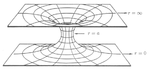
Figure 1: One black hole

This manifold has two ends, one for $r\rightarrow\infty$ and one for $r\rightarrow 0$. They have the same geometry and hence the same ADM mass, as it must be the case since individual and total mass clearly coincide for a single hole.

The data just written down correspond to the ‘middle’ slice right across the Kruskal (maximally extended Schwarzschild) manifold. Also, (43) is just the spatial part of the Schwarzschild metric in isotropic coordinates. Hence we know its entire future development in analytic form. Already for two holes this is not the case anymore. Even the simplest two body problem—head-on collision— has not been solved analytically in GR.

5.5.2 Two black holes

There is an obvious generalization of (42) by allowing two ‘monopoles’ of strength $a_{1}$ and $a_{2}$ at the punctures $\vec{x}=\vec{x}_{1}$ and $\vec{x}=\vec{x}_{2}$ respectively. The 3-metric then reads

$$ds^{2}=\left(1+\frac{a_{1}}{|\vec{x}-\vec{x}_{1}|}+\frac{a_{2}}{|\vec{x}-\vec{x}_{2}|}\right)^{4}(dr^{2}+r^{2}\,d\theta^{2}+\sin^{2}\theta\,d\varphi^{2}).$$ (46)

The manifold has now three asymptotically flat ends, one for $|\vec{x}|\rightarrow\infty$, where the overall ADM mass $M$ is measured, and one each for $|\vec{x}-\vec{x}_{1,2}|\rightarrow 0$. To see the latter, it is best to write the metric (46) in spherical polar coordinates $(r_{1},\theta_{1},\varphi_{1})$ centered at $\vec{x}_{1}$, and then introduce the inverted radial coordinate given by $\bar{r}_{1}=a_{1}^{2}/r_{1}$. In the limit $\bar{r}_{1}\rightarrow\infty$ the metric then takes the form

$$ds^{2}=\left(1+\frac{a_{1}(1+a_{2}/r_{12})}{\bar{r}_{1}}+O((1/\bar{r}_{1})^{2})\right)^{4}(d\bar{r}^{2}+\bar{r}^{2}\,(d\theta_{1}^{2}+\sin^{2}\theta_{1}d\varphi_{1}^{2}))$$ (47)

where $r_{12}=|\vec{x}_{1}-\vec{x}_{2}|$. This looks just like a one-hole metric (43). Hence, if the black holes are well separated (compared to their size), the two-hole geometry looks like that depicted in figure 2.

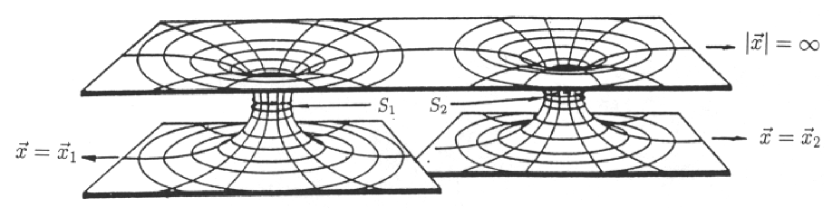
Figure 2: Two black holes well separated

By comparison with the one-hole metric we can immediately write down the ADM masses corresponding to the three ends $r,\bar{r}_{1,2}\rightarrow\infty$ respectively:

$$M=2(a_{1}+a_{2}),\quad m_{1,2}=2a_{1,2}(1+\chi_{1,2}),\quad\mbox{where}\quad\chi_{1,2}=\frac{a_{2,1}}{r_{12}}\,.\qquad$$ (48)

Momenta and angular momenta clearly vanish (moment of time symmetry). Still assuming well separated holes, i.e. $\chi_{i}=a_{i}/r_{12}\ll 1$, we can calculate the binding energy $\Delta E=M-m_{1}-m_{2}$ as function of the masses $m_{i}$ and $r_{12}$ and get

$$\Delta E=-\frac{m_{1}m_{2}}{r_{12}}\left(1-\frac{m_{1}+m_{2}}{2r_{12}}+O((m_{1,2}/r_{12})^{2})\right)\,.$$ (49)

The leading order is just the Newtonian expression for the binding energy of two point-particles with masses $m_{1,2}$ at distance $r_{12}$. But there are corrections to this Newtonian form which tend to diminish the Newtonian value. Note also that (49) is still not in a good form since $r_{12}$ is not an invariantly defined geometric distance measure. As such one might use the length $\ell$ of the shortest geodesic joining the two apparent horizons $S_{1}$ and $S_{2}$. Unfortunately these horizons are not easy to locate analytically and hence no closed form of $\ell(m_{1},m_{2},r_{12})$ exists which could be inverted to eliminate $r_{12}$ in favour of $\ell$.

Due to the difficulty to analytically locate the two apparent horizons we also cannot write down an analytic expression for their area. But we can give upper and lower bounds as follows:

$$16\pi(2a_{i})^{2}<A_{i}<16\pi[(2a_{i}(1+\chi_{i})]^{2}=16\pi m_{i}^{2}\,.$$ (50)

The lower bound simply follows from the fact that the two-hole metric (46), if written down in terms of spherical polar coordinates about any of its punctures, equals the one hole metric (43) plus a positive definite correction. The upper bound follows from the so-called Penrose inequality in Riemannian Geometry (proven in [27]), which directly states that $16\pi m^{2}\geq A$ for each asymptotically flat end, where $m$ is the mass according to (35) and $A$ is the area of the outermost (as seen from that end) minimal surface.

If the two holes approach each other to a distance comparable to the sizes of the holes the geometry changes in an essential way. This is shown in figure 3.

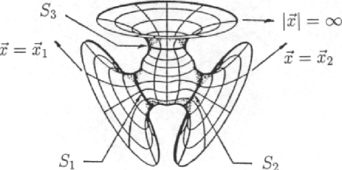
Figure 3: Two black holes after merging

The most important new feature is that new minimal surfaces form, in fact two [10], which both enclose the two holes. The outermost of these, as seen from the upper end, denoted by $S_{3}$ in figure 3, corresponds to the apparent horizon of the newly formed ‘compound’ black hole which contains the two old ones. For two black holes of equal mass, i.e. $a_{1}=a_{2}=a$, this happens approximately for a parameter ratio of $a/r_{12}=0.65$, which in an approximate numerical translation into the ratio of individual hole mass to geodesic separation reads $m/\ell\approx 0.26$.

5.5.3 More than two black holes

The method can be generalized in a straightforward manner to any number $n$ of black holes with parameters $(a_{i},\vec{x}_{i})$, $i=1,\cdots n$, for the punctures. The manifold $\Sigma$ has now $n+1$ ends, one for $|\vec{x}|\rightarrow\infty$ and one for each $\vec{x}\rightarrow\vec{x}_{i}$. The expressions for the metric and masses are then given by the obvious generalizations of (46) and (48) respectively.

5.5.4 Energy bounds from Hawking’s area law

Loosely speaking, Hawking’s area law states that the surface of a black hole cannot decrease with time. (See [23] for a simple and complete outline of the traditional and technically slightly restricted version and [9] for the technically most complete proof known today.) Let us briefly explain this statement. If $\Sigma$ is a Cauchy surface (a spacelike hypersurface in spacetime) and $\mathcal{H}$ the event horizon (a lightlike hypersurface in spacetime), the two intersect in a number of components (spacelike 2-manifolds), each of which we assume to be a two-sphere. Each such two-sphere is called the surface of a black hole at time $\Sigma$. Let us pick one of them and call it $B$. Consider next a second Cauchy surface $\Sigma^{\prime}$ which lies to the future of $\Sigma$. The outgoing null rays of $B$ intersect $\Sigma^{\prime}$ in a surface $B^{\prime}$, and the statement is now that the area of $B^{\prime}$ is larger than or equal to the area of $B$ (to prove this one must assume the strong energy condition). Note that we deliberately left open the possibility that $B^{\prime}$ might be a proper subset of a black hole surface at time $\Sigma^{\prime}$, namely in case the original hole has merged in the meantime with another one. If this does not happen $B^{\prime}$ may be called the surface of the same black hole at the later time $\Sigma$.

Following an idea of Hawking’s [24], this can be applied to the future evolution of multi black hole data as follows. As we already mentioned, the event horizon lies on or outside the apparent horizon. Hence the area of the ‘surface’ (as just defined) of a black hole is bounded below by the area of the corresponding apparent horizon, which in turn has the lower bound stated in (50). Suppose that after a long time our configuration settles in an approximately stationary state, at least for some interior region where no gravitational radiation is emitted anymore. Since our data have zero linear and angular momentum, the final state is static and uniquely given by a single Schwarzschild hole of some final mass $M_{\rm\scriptscriptstyle final}$ and corresponding surface area $A_{\rm\scriptscriptstyle final}=16\pi M_{\rm\scriptscriptstyle final}^{2}$. This is a direct consequence of known black hole uniqueness theorems (see [26] or p. 157-186 of [25] for a summary). By the area theorem $A_{\rm\scriptscriptstyle final}$ is not less than the sum of all initial apparent horizon surface areas. This immediately gives

$$M_{\rm\scriptscriptstyle final}\geq\sqrt{\sum_{i}A_{i}^{\rm\scriptscriptstyle initial}/16\pi}\geq 2\sqrt{\sum_{i}^{n}a_{i}^{2}}\,.$$ (51)

In passing we remark that applied to a single black hole this argument shows that it cannot lose its mass below the value $m_{\scriptscriptstyle\rm ir}:=\sqrt{A^{\rm\scriptscriptstyle initial}/16\pi}$, called its irreducible mass. Back to the multi-hole case, the total initial mass is given by the straightforward generalization of (48):

$$M_{\rm\scriptscriptstyle initial}=\sum_{i}m_{i}=2\sum_{i}a_{i}(1+\chi_{i}),\quad\mbox{where}\quad\chi_{i}=\sum_{i\not=k}\frac{a_{k}}{|\vec{x}_{i}-\vec{x}_{k}|}\,.$$ (52)

Using these two equations we can write down a lower bound for the fractional energy loss into gravitational radiation:

$$\frac{\Delta M}{M}:=\frac{M_{\rm\scriptscriptstyle initial}-M_{\rm\scriptscriptstyle final}}{M_{\rm\scriptscriptstyle initial}}\leq 1-\frac{\sqrt{\sum_{i}a_{i}^{2}}}{\sum_{i}a_{i}(1+\chi_{i})}\,.$$ (53)

For a collision of $n$ initially widely separated ($\chi_{i}\rightarrow 0$) holes of equal mass this becomes

$$\frac{\Delta M}{M}=1-\sqrt{1/n}\,.$$ (54)

For just two holes this means that at most 29% of their total rest mass can be radiated away. But this efficiency can be enhanced if the energy is distributed over a larger number of black holes.

Another way to raise the upper bound for the efficiency is to consider spinning black holes. For two holes the maximal value of 50% can be derived by starting with two extremal black holes (i.e. of maximal angular momentum: $J=m^{2}$ in geometric units) which merge to form a single unspinning black hole [24].

One can also envisage a situation where one hole participates in a scattering process but does not merge. Rather it gets kicked out of the collision zone and settles without spin (for simplicity) in an quasistationary state (for some time) far apart. The question is what fraction of energy the area theorem allows it to lose. Let this be the $k$th hole. Then $m^{\rm\scriptscriptstyle final}_{k}\geq 2a_{k}=m^{\rm\scriptscriptstyle initial}_{k}/(1+\chi_{k})$. Hence

$$\frac{m^{\rm\scriptscriptstyle initial}_{k}-m^{\rm\scriptscriptstyle final}_{k}}{m^{\rm\scriptscriptstyle initial}_{k}}\leq\frac{\chi_{k}}{1+\chi_{k}}<1\,,$$ (55)

showing that an appreciable efficiency can only be obtained if the data are such that $\chi_{k}$ is not too close to zero. This means that the $kth$ hole was originally not too far from the others. This seems an unlikely process. Hence it is difficult to extract energy from a single unspinning hole.

For a single spinning black hole the situation is again different. Spinning it down from an extreme state to zero angular momentum sets an upper bound for the efficiency from the area law of 29%. This follows easily from the following relation between mass, irreducible mass, and angular momentum for a Kerr black hole (see e.g. [32], formula (33.60)):

$$m^{2}=m_{\scriptscriptstyle\rm ir}^{2}+J^{2}/4m_{\scriptscriptstyle\rm ir}^{2}$$ (56)

Setting $J=m^{2}$ one solves for $m_{\scriptscriptstyle\rm ir}/m=\sqrt{1/2}$; hence $(m-m_{\scriptscriptstyle\rm ir})/m=1-\sqrt{1/2}\approx 0.29$. It can moreover be shown [8] that this limit can be (theoretically) realised by the Penrose process (compare Frolov’s lecture).

Needless to say that realistic processes may have far less efficiency than this theoretical bounds from the area law alone indicate. Recent numerical studies of the head-on (i.e. zero angular momentum) collision of two equal-mass black holes give a radiated energy in units of the total energy of only $10^{-3}$ [3]. With angular momentum the efficiency is of course expected to be much better. Here recent numerical investigations give an estimate of $3\times 10^{-2}$ for an inspiral of two equal-mass non-spinning black holes from the innermost stable circular orbit [2]: still a long way from the theoretical upper bound.

5.5.5 Other topologies

Other topologies can be found which support initial data with apparent horizons. For example, instead of the ‘Schwarzschild’ manifold with $n+1$ ends for $n$ black holes one can find one which has just two ends for any number $\geq 2$ of holes and which has been termed the Einstein-Rosen manifold [29].

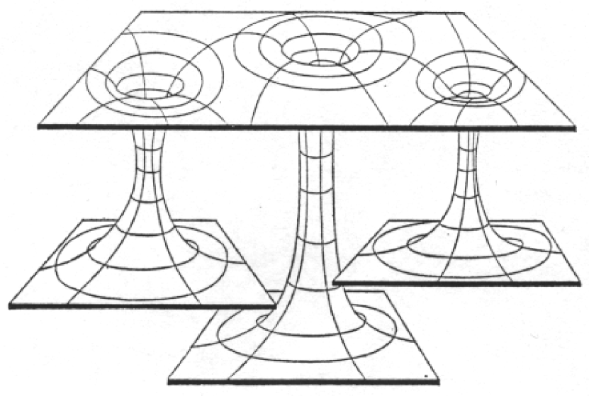
Figure 4: Multi-Schwarzschild

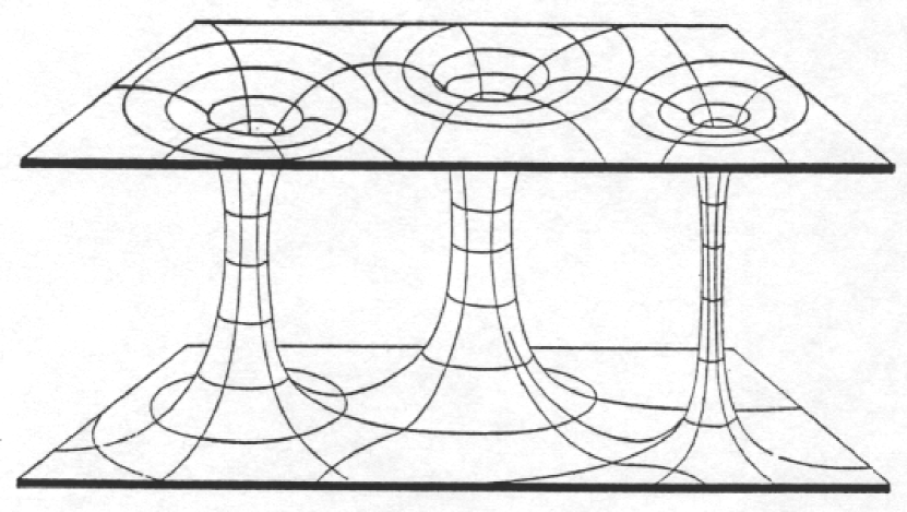
Figure 5: Einstein-Rosen manifold

The difference to the data already discussed does not primarily lie in the physics they represent. After all their different topologies are hidden behind event horizons for the outside observer, even though their interaction energies are slightly different [20][22]. However, the point we wish to stress here is that such data can analytically and numerically be more convenient, despite the fact that the underlying manifold might seem topologically more complicated. The reason is that these data have more symmetries, and that coordinate systems can be found for which these symmetries take simple analytic expressions. For example, in the Einstein-Rosen manifold the upper and lower ends are isometrically related by reflections about the minimal 2-spheres in each connecting tube, with the fixed-point sets being the apparent horizons. Hence all the apparent horizons can analytically be easily located in the multi-hole Einstein-Rosen manifold, in contrast to the multi-hole Schwarzschild manifold.

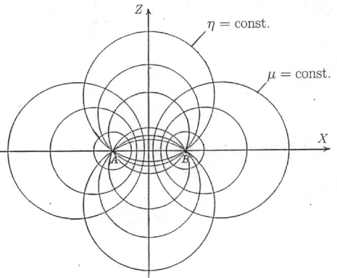
Figure 6: bipolar coordinates

Let us briefly explain this for two holes of equal mass. Here one starts again from $\mathbb{R}^{3}$ coordinatised by spherical bi-polar coordinates. These are obtained from bi-polar coordinates $(\mu,\eta)$ in the $xz$ plane by adding an azimuthal angle $\varphi$ corresponding to a rotation about the $z$ axis, just like ordinary spherical polar coordinates are produced from ordinary polar coordinates in the $xz$-plane. The coordinates $(\mu,\eta)$ parametrise the $xz$-plane according to $\exp(\mu-i\eta)=(\xi+c)/(\xi-c)$, where $\xi=z+ix$ and $c>0$ is a constant. The lines of constant $\mu$ intersect those of constant $\eta$ orthogonally. Both families consist of circles; those in the first family are centered on the $z$-axis with radii $c/\sinh\mu$ at $z=c\,\coth\mu$, and those in the second family on the $x$-axis with radii $c/|\sin\eta|$ at $|x|=c\,\cot\eta$.

Following an idea of Misner [31], one can borrow the method of images from electrostatics (see. e.g. chapter 2.1 in [28]) to construct solutions $\Phi$ to the Laplace equation such that the metric $h_{ij}=\Phi^{4}\delta_{ij}$ has a number of reflection isometries about two-spheres, one for each hole. In the two hole case one uses the two two-spheres $\mu=\pm\mu_{0}$ for some $\mu_{0}>0$, which then become the apparent horizons. Using these isometries we can take two copies of our initial manifold, excise the balls $|\mu|>\mu_{0}$ and glue the two remaining parts ‘back to back’ along the two boundaries $\mu=\mu_{0}$ and $\mu=-\mu_{0}$. The isometry-property is necessary so that the metric continues to be smooth across the seam. This gives an Einstein-Rosen manifold with two tubes (or ‘bridges’, as they are sometimes called) connecting two asymptotically flat regions.

In fact, we could have just taken one copy of the original manifold, excised the balls $|\mu|>\mu_{0}$, and mutually glued together the two boundaries $\mu=\pm\mu_{0}$. This also gives a smooth metric across the seam and results in a manifold known as the Misner wormhole [30].

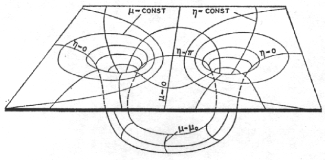
Figure 7: The Misner Wormhole representing two black holes

Metrically the Misner wormhole is locally isometric to the Einstein-Rosen manifold with two tubes (which is its ‘double cover’), but their topologies obviously differ. This means that for the observer outside the apparent horizons these two data sets are indistinguishable. This is not quite true for the Einstein-Rosen and Schwarzschild data, which are not locally isometric. Even without exploring the region inside the horizons (which anyway is rendered impossible by existing results on topological censorship [16]) they slightly differ in their interaction energy and other geometric quantities, like e.g. the tidal deformation of the apparent horizons.

The two parameters $c$ and $\mu_{0}$ now label the two-hole configurations of equal mass. (In the Schwarzschild case the two independent parameters were $a\equiv a_{1}=a_{2}$ and $r_{12}\equiv|\vec{x}_{1}-\vec{x}_{2}|$.) But unlike the Schwarzschild case, we can now give not only closed analytic expressions for the total mass $M$ and individual mass $m$ in terms of the two parameters, but also for the geodesic distance of the apparent horizons $\ell$. ($\ell$ is used as definition for ‘instantaneous distance of the two black holes’; for the Misner wormhole, where the two apparent horizons are identified, this corresponds to the length of the shortest geodesic winding once around the wormhole.) These read

$$M=4c\sum_{n=1}^{\infty}\frac{1}{\sinh n\mu_{0}},\quad m=2c\sum_{n=1}^{\infty}\frac{n}{\sinh n\mu_{0}},\quad\ell=2c(1+2m\mu_{0}).$$ (57)

You might rightly wonder what ‘individual mass’ should be if there is no internal end associated to each black hole where the ADM-formula (35) can be applied. The answer is that there are alternative definitions of ‘quasi-local-mass’ which can be applied even without asymptotic ends. The one we used for the expression of $m$ above is due to Lindquist [29] and is easy to compute in connection with the method of images. But it is lacking a deeper mathematical foundation. An alternative which is mathematically better founded is due to Penrose [34], which however is much harder to calculate and only applies to a limited set of situations (it agrees with the ADM mass whenever both definitions apply). Amongst them are, however, all time-symmetric conformally flat data, and for the data above the Penrose mass has fortunately been calculated in [36]. The expression for $m$ is rather complicated and differs from that given above, though the difference is only of sixth order in an expansion in (mass/distance) [20].

In summary, we see that the problem of setting up initial data for two black holes of given individual mass and given separation has no unique answer. Metrically as well as topologically different data sets can be found which have the same right to be called a realization of such a configuration. For holes without associated asymptotically flat ends no unambiguous definition for quasi-local mass exists.

5.6 Non time-symmetric data

According to a prescription found by Bowen and York [37], we can add linear and angular momentum within the setting of maximal data. We can still use conformally flat data, i.e. set $\hat{h}_{ij}=\delta_{ij}$, on multiply punctured $\mathbb{R}^{3}$. Then the following two expressions add linear momentum $P^{i}$ and spin angular momentum $S^{i}$ to the puncture $\vec{x}=\vec{0}$:

$$\hat{K}_{P}^{ij} = \frac{3}{2r^{2}}\left(P^{i}n^{j}+P^{j}n^{i}-(\delta^{ij}-n^{i}n^{j})(\vec{P}\cdot\vec{n})\right)\,,$$ (58)

$$\hat{K}_{S}^{ij} = \frac{3}{r^{3}}((\vec{S}\times\vec{n})^{i}n^{j}+(\vec{S}\times\vec{n})^{j}n^{i})\,.$$ (59)

It is straightforward to check that these expressions satisfy (38) (note that $\hat{D}_{i}=\partial_{i}$). One can also check that these data will indeed give the proposed momenta and angular momenta at infinity (i.e. at the end $r\rightarrow\infty$). For this one may just use the ‘hatted’ quantities in (36) and (37), since the rescaling (41) does not influence the leading order parts in the $1/r$ expansion of $K$, which alone contribute to these integrals. Linearity of all these equations in $K$ allows us to just add $K_{P}$ and $K_{S}$ and get initial data for one black hole with given momentum $\vec{P}$ and (spin) angular momentum $\vec{S}$. Moreover, we can add any finite number of expressions of the kind (58 and 59) with parameters ${\vec{P}}_{i},{\vec{S}}_{i}$ based at the puncture $\vec{x}_{i}$, where $i=1,\cdots,n$. This then leads to a data set whose total linear and angular momentum is given by the sum $\sum_{i}{\vec{P}}_{i}$ and $\sum_{i}{\vec{S}}_{i}$ respectively. But one may not immediately conclude that the ${\vec{P}}_{i}$ and ${\vec{S}}_{i}$ are linear and angular momenta of the individual black holes. Rather, the latter must be calculated for the internal ends of the manifold and for this one needs to know $\Phi$. The task then remains to solve (39) for the conformal factor, with blow-ups being allowed at the given punctures.

One interesting idea to facilitate solving (39) is to first split off the singular part of $\Phi$, which blows up at the punctures $\{\vec{x}_{1},\cdots,\vec{x}_{n}\}$ like $1/|\vec{x}-\vec{x}_{i}|$, from the regular reminder [6] (compare also [5]). One writes

$$\Phi=\frac{1}{\alpha}+U,\quad\mbox{with}\quad\frac{1}{\alpha}:=\sum_{i=n}^{n}\frac{a_{i}}{|\vec{x}-\vec{x}_{i}|}\,,$$ (60)

where the $a_{i}>0$ may be freely prescribed. Inserting this into (39) gives

$$\Delta U+\beta(1+\alpha U)^{-7}=0,\quad\mbox{with}\quad\beta=\hbox{${\textstyle{\frac{1}{8}}}$}\alpha^{7}K^{ij}K_{ij}\,.$$ (61)

The point is now the following: for $\vec{x}\rightarrow\vec{x}_{i}$ the function $\alpha$ tends to zero as $|\vec{x}-\vec{x}_{i}|$; hence $\beta$, too, tends to zero as $|\vec{x}-\vec{x}_{i}|$. This means that (61) has continuous coefficients everywhere in $\mathbb{R}^{3}$ since the $1/|\vec{x}-\vec{x}_{i}|^{6}$–singularity at $\vec{x}_{i}$ of the $K$-squared term is cancelled by multiplication with $\alpha^{7}$. (Note that this relies on using the $K$’s from (58, 59), which possess no $1/r^{n}$ terms with $n>3$.) This means that equation (61) for $U$ can be solved on all of $\mathbb{R}^{3}$, without the need to excise the points $\{\vec{x}_{1},\cdots,\vec{x}_{n}\}$ and therefore without the need to specify ‘inner’ boundary conditions for $U$; only the ‘outer’ boundary-condition $U(r\rightarrow\infty)\rightarrow 1$ remains. This simplification seems particularly useful in numerical implementations (compare [6]).

The total mass of our configuration is $M=\sum_{i}2a_{i}$. The individual masses are determined just as in 5.5.2, by introducing the inverted radial coordinate $\bar{r}_{i}=a_{i}^{2}/r_{i}$ and reading off the coefficient of the $1/2\bar{r}_{i}$ term in the $\bar{r}_{i}\rightarrow\infty$ expansion. One easily gets

$$m_{i}=2a_{i}(U(\vec{x}_{i})+\chi_{i})$$ (62)

with $\chi_{i}$ as in (52).

The linear and angular momenta at, say, the $k$th end can also be calculated by using inverted coordinates, given by $\vec{\bar{x}}=(\vec{x}-{\vec{x}}_{k})a^{2}_{k}/r^{2}_{k}$. Expressed in these coordinates, the ‘hatted’ (unphysical) extrinsic curvature tensor is given by $J^{i}_{k}J^{j}_{l}\hat{K}_{ij}$ where $J^{i}_{k}:=\frac{\partial x^{i}}{\partial{\bar{x}^{k}}}=(a^{2}_{k}/\bar{r}^{2})R^{i}_{k}$ with $R^{i}_{k}=\delta^{i}_{k}-2n^{i}n_{k}$, which is an orthogonal matrix. The ‘physical’ extrinsic curvature is then obtained by multiplication with $\Phi^{-2}$ (compare 41). Now, $\Phi(\vec{\bar{x}})=\frac{\bar{r}}{a_{k}}(1+\frac{m_{k}}{2\bar{r}}+O((1/\bar{r})^{2}))$ so that

$$\bar{K}_{ij}=\left\{\bigl{(}\frac{a_{k}}{\bar{r}}\bigr{)}^{6}+\mbox{terms}\propto\bigl{(}\frac{a_{k}}{\bar{r}}\bigr{)}^{p}\right\}(R^{k}_{i}R^{l}_{j}\hat{K}_{kl}),\quad\mbox{where}\quad p\geq 7\,.$$ (63)

Inserting the expression (58) for $\hat{K}_{P}$ results in a $1/{\bar{r}}^{4}$ falloff so that the individual linear momenta are all zero as measured from the internal ends. One may say that the asymptotically flat internal ends represent the local rest frames of the black holes. Note that these rest frames are inertial since each black hole is freely falling. Inserting $K_{S}$ from (59) gives a $1/{\bar{r}}^{3}$ falloff and an angular momentum which is just $-{\vec{S}}_{k}$ for the $k$th end. (Here one uses that $R^{i}_{k}$ is orientation-reversing orthogonal, hence changing the sign of $\varepsilon_{ijk}$, and that $R^{i}_{k}(\vec{S}\times\vec{n})^{k}=-(\vec{S}\times\vec{n})^{i}$.)

6 Problems and recent developments

In this final section we draw attention to some of the current problems and developments, without claiming completeness.

1. Given black hole data for $n$ holes of fixed masses and mutual separations (whatever definitions one uses here). One would like to minimize these data on the amount of outgoing radiation energy. Any excess over the minimal amount can be said to be ‘already contained’ initially. But so far no local (in time) criterion is known which quantifies the amount of gravitational radiation in an initial data set. First hints at the possibility that some (Newman-Penrose) conserved quantities could be useful here were discussed in [13].

2. Restricting to spatially conformally flat metrics seems to be too narrow. It has been shown that there are no conformally flat spatial slices in Kerr spacetime which are axisymmetric and reduce to slices of constant Schwarzschild time in the limit of vanishing angular momentum [18]. Accordingly, Bowen-York data, even for a single black hole, contain excess gravitational radiation due to the relaxation of the individual holes to Kerr form [19]. See also [33] for an informal discussion of this and related problems. An alternative to the Bowen-York data which describe two spinning black holes and which reduce to Kerr data if the mass of one hole goes to zero have been discussed in [12].

3. Even for the most simple 2-hole data (Schwarzschild or Einstein-Rosen) it is not known whether the evolving spacetime will have a suitably smooth asymptotic structure at future-lightlike infinity (i.e. ‘scri-plus’). As a consequence, we still do not know whether we can give a rigorous mathematical meaning to the notion of ‘energy loss by gravitational radiation’ in this case of the simplest head-on collision of two black holes! The difficult analytical problems involved are studied in the framework of the so-called ‘conformal field equations’. See [17] (in particular section 4) for a summary and references.

4. We usually like to ask ‘Newtonian’ questions, like: given two black holes of individual masses $m_{1,2}$ and mutual separation $\ell$, what is their binding energy? For such a question to make sense we need good concepts of quasi-local mass and distance. But these are ambiguous concepts in GR. Different definitions of ‘quasi-local mass’ and ‘distance’ amount to differences in the calculated binding energies which can be a few $10^{-3}$ times total energy at closest encounter [20]. This is of the same order of magnitude as the total energy lost into gravitational radiation found in [3] for head-on (i.e. zero angular momentum) collision of two black holes modelled with Misner data.

7 Appendix: Eq. (2) satisfies the energy principle

By the ‘energy principle’ we understand the property, that all energy of the self-gravitating system serves as source for the gravitational field. In this appendix we wish to prove that (2) indeed satisfies this principle. For the uniqueness argument see [21].

Given a matter distribution $\rho$ immersed in its own gravitational potential $\phi$. Suppose we redistribute the matter within a bounded region of space by actively dragging it along the flow lines of a vector field $\vec{\xi}$ which vanishes outside some bounded region. The rate of change, $\delta\rho$, of the matter distribution is then determined through $\delta\rho\,dV=-L_{\vec{\xi}}\,(\rho\,dV)=-\vec{\nabla}\cdot(\vec{\xi}\rho)\,dV$, where $L_{\vec{\xi}}$ is the Lie derivative with respect to $\vec{\xi}$ and $dV$ is the standard spatial volume element. Note that the latter also needs to be differentiated along $\vec{\xi}$, resulting in $L_{\vec{\xi}}\,dV=\vec{\nabla}\cdot\vec{\xi}$. Hence we have $\delta\rho=-\vec{\nabla}\cdot(\vec{\xi}\rho)$. The rate of work done to the system during this process is

$$\delta A=\int_{\mathbb{R}^{3}}dV\,\rho\vec{\xi}\cdot\vec{\nabla}\phi=-\int_{\mathbb{R}^{3}}dV\,\phi\,\vec{\nabla}\cdot(\vec{\xi}\rho)=\int_{\mathbb{R}^{3}}dV\,\phi\,\delta\rho\,,$$ (64)

where the integration by parts does not lead to surface terms due to $\vec{\xi}$ vanishing outside a bounded region. Equation (64) is still completely general, that is, independent of the field equation for $\phi$. The field equation comes in when we assume that the process of redistribution is carried out adiabatically, which means that at each stage during the process $\phi$ satisfies its field equation with the instantaneous matter distribution. Our claim will be proven if under the hypothesis that $\phi$ satisfies (2) we can show that $\delta A=c^{2}\delta M_{G}$, where $M_{G}$ is defined in (5) and represents the total gravitating energy according to the field equation. Setting $\sqrt{\phi/c^{2}}=\psi$ and using the more convenient equation (3), we have

$$\delta A = \frac{c^{4}}{2\pi G}\int_{\mathbb{R}^{3}}dV\,\psi^{2}\delta\left[\frac{\Delta\psi}{\psi}\right]=\frac{c^{4}}{2\pi G}\int_{\mathbb{R}^{3}}dV\,\left[\psi\Delta(\delta\psi)-(\Delta\psi)\delta\psi\right]$$ (65)

$$= \frac{c^{4}}{2\pi G}\,\lim_{r\rightarrow\infty}\int_{S^{2}(r)}d\sigma\,\vec{n}\cdot\left[\psi\vec{\nabla}(\delta\psi)-(\vec{\nabla}\psi)\delta\psi\right]\,.$$

Now, the fall-off condition for $r\rightarrow\infty$ imply that $\vec{\nabla}\psi$ falls off as fast as $1/r^{2}$ and $\delta\psi$ as $1/r$. Hence the second term in the last line of (65) does not contribute so that we may reverse its sign. This leads to

$$\delta A = \frac{c^{4}}{2\pi G}\,\delta\,\lim_{r\rightarrow\infty}\int_{S^{2}(r)}d\sigma\,(\vec{n}\cdot\vec{\nabla}\psi)\psi=\frac{c^{4}}{4\pi G}\,\delta\,\lim_{r\rightarrow\infty}\int_{S^{2}(r)}d\sigma\,\vec{n}\cdot\vec{\nabla}\phi$$ (66)

$$= c^{2}\delta M_{G}$$

which proves the claim.

References

- [1] Arnowitt R and Deser S and Misner C 1961 “Coordinate invariance and energy expressions in general relativity” Phys. Rev. 122 997-1006
- [2] Baker J et al. 2001 “Plunge waveforms from inspiralling binary black holes” Phys. Rev. Lett. 87 121103 (gr-qc/0102037)
- [3] Baker J et al. 2000 “Gravitational waves from black hole collisions via an eclectic approach” Class. Quant. Grav. 17 L149-L156
- [4] Beig R and Ó Murchadha N 1987 “The Poincaré group as the symmetry group of canonical general relativity”. Ann. Phys. (NY) 174 463-498
- [5] Beig R 2000 “Generalized Bowen–York initial data” in: Cotsakis S and Gibbons G (eds.) Mathematical and Quantum Aspects of Relativity and Cosmology Lecture Notes In Physics, Vol. 537 (Berlin: Springer-Verlag) (gr-qc/0005043)
- [6] Brandt S and Brügmann B 1997 “A simple construction of initial data for multiple black holes” Phys. Rev. Lett. 78 3606-3609 (gr-qc/9703066)
- [7] Choquet-Bruhat Y and Geroch R 1969 “Global aspects of the Cauchy problem in general relativity” Comm. Math. Phys. 3 334–357
- [8] Christodoulou D 1970 “Reversible and irreversible transformations on black-hole physics” Phys. Rev. Lett. 25 1596-1597
- [9] Chruściel P et al. 2001 “The area theorem”, Annales Henri Poincaré 2 109-178 (gr-qc/0001003)
- [10] Čadež A. 1974 “Apparent horizons in the two-black hole problem” Ann. Phys. (NY) 83 449–457
- [11] Dadhich N and Narlikar J (eds.) 1998 Gravitation and Relativity: At the turn of the Millenium Proceedings of the GR-15 Conference, held at IUCAA, Pune, India, Dec. 1997; published by IUCAA.
- [12] Dain S 2001 “Initial data for two Kerr-like black holes” Phys. Rev. Lett. 87 121102 (gr-qc/0012023)
- [13] Dain S and Valiente-Kroon J A 2002 “Conserved quantities in a black hole collision” Class. Quant. Grav. 19 811-816 (gr-qc/0105109)
- [14] Damour T 1987 “The problem of motion in Newtonian and Einsteinian gravity” in : Hawking S and Israel W 300 Years of Gravitation pp. 128-198 (Cambridge: Cambridge University Press)
- [15] Ehlers J et al. 1976 “Comments on gravitational radiation damping and energy loss in binary systems” Astroph. J. 208 L77-L81
- [16] Friedman J et al. 1993 “Topological censorship” Phys. Rev. Lett. 71 1486-1489; Erratum-ibid. 75 (1995) 1872
- [17] Friedrich H 1998 “Einstein’s equation and geometric asymptotics” in: [11] pp. 153-176 (gr-qc/9804009)
- [18] Garat A and Price R 2000 “Nonexistence of conformally flat slices of the Kerr spacetime” Phys. Rev. D61 124011 (gr-qc/0002013)
- [19] Gleiser R et al. 1998 “Evolving the Bowen-York initial data for spinning black holes” Phys. Rev. D57 3401-3407 (gr-qc/9710096)
- [20] Giulini D 1990 “Interaction energies for three-dimensional wormholes” Class. Quant. Grav. 7 1271-1290
- [21] Giulini D 1996 “Consistently implementing the fields self-energy in Newtonian gravity” Phys. Lett. A232 165-170 (gr-qc/9605011)
- [22] Giulini D 1998 “On the construction of time-symmetric black hole initial data” in: Hehl et al. (1998) p 224-243
- [23] Giulini D 1998 “Is there a general area theorem for black holes?” J. Math. Phys. 39 6603-6606
- [24] Hawking S 1971 “Gravitational radiation from colliding black holes” Phys. Rev. Lett. 26 1344-1346
- [25] Hehl F et al. (eds.) 1998 Black Holes: Theory and Observation, Lecture Notes in Physics Vol. 514 (Berlin: Springer-Verlag)
- [26] Heusler M 1996 Black Hole Uniqueness Theorems, Cambridge Lecture Notes in Physics (Cambridge: Cambridge University Press)
- [27] Huisken G and Ilmanen T 1997 “The Riemannian Penrose Inequality” Int. Math. Res. Not. 20 1045-1058
- [28] Jackson J D 1975 Classical Electrodynamics (second edition) (New York: John Wiley & Sons)
- [29] Lindquist R W 1963 “Initial-value problem on Einstein-Rosen manifolds” J. Math. Phys. 4 938-950
- [30] Misner C 1960 “Wormehole initial conditions” Phys. Rev. 118 1110–1111
- [31] Misner C 1963 “The method of images in geometrostatics” Ann. Phys. (NY) 24 102-117
- [32] Misner C W and Thorne K S and Wheeler J A 1973 Gravitation (New York: W H Freeman & Comp.)
- [33] Pullin J 1998 “Colliding black holes: analytic insights” in [11] pp. 87-105 (gr-qc/9803005)
- [34] Penrose R 1982 “Quasi-local mass and angular momentum in general relativity” Proc. Roy. Soc. Lond. A 381 53-63
- [35] Smarr L (ed.) 1997 Sources of gravitational radiation (Cambridge: Cambridge University Press)
- [36] Tod K.P. 1983 “Some examples of Penrose’s quasi-local mass construction” Proc. Roy. Soc. Lond. A 388 457-477
- [37] York J 1979 “Kinematics and dynamics of general relativity” in: Smarr L (1979) p 83-126