Anisotropic Relativistic Stellar Models

Abstract

We present a class of exact solutions of Einstein’s gravitational field equations describing spherically symmetric and static anisotropic stellar type configurations. The solutions are obtained by assuming a particular form of the anisotropy factor. The energy density and both radial and tangential pressures are finite and positive inside the anisotropic star. Numerical results show that the basic physical parameters (mass and radius) of the model can describe realistic astrophysical objects like neutron stars.

PACS Numbers: 97.10 Cv, 97.60 Jd, 04.20.Jb

Keywords: Anisotropic Stars; Einstein’s field equations; Static interior solutions.

I Introduction

Since the pioneering work of Bowers and Liang [1] there is an extensive literature devoted to the study of anisotropic spherically symmetric static general relativistic configurations. The study of static anisotropic fluid spheres is important for relativistic astrophysics. The theoretical investigations of Ruderman [2] about more realistic stellar models show that the nuclear matter may be anisotropic at least in certain very high density ranges ($\rho>10^{15}g/cm^{3}$), where the nuclear interactions must be treated relativistically. According to these views in such massive stellar objects the radial pressure may not be equal to the tangential one. No celestial body is composed of purely perfect fluid. Anisotropy in fluid pressure could be introduced by the existence of a solid core or by the presence of type $3A$ superfluid [3], different kinds of phase transitions [4], pion condensation [5] or by other physical phenomena. On the scale of galaxies, Binney and Tremaine [6] have considered anisotropies in spherical galaxies, from a purely Newtonian point of view. Other source of anisotropy, due to the effects of the slow rotation in a star, has been proposed recently by Herrera and Santos [7].

The mixture of two gases (e.g., monatomic hydrogen, or ionized hydrogen and electrons) can formally be also described as an anisotropic fluid [8]. More generally, when the fluid is composed of two fluids the total energy-momentum tensor is

$$T^{ik}=\left(P_{1}+\rho_{1}\right)U^{i}U^{k}-P_{1}g^{ik}+\left(P_{2}+\rho_{2}\right)W^{i}W^{k}-P_{2}g^{ik},$$ (1)

where $U_{i}U^{i}=1$ and $W_{i}W^{i}=1$. By means of the transformations

$$U^{\ast i}=U^{i}\cos\alpha+\sqrt{\frac{P_{2}+\rho_{2}}{P_{1}+\rho_{1}}}W^{i}\sin\alpha,W^{\ast i}=-\sqrt{\frac{P_{2}+\rho_{2}}{P_{1}+\rho_{1}}}U^{i}\sin\alpha+W^{i}\cos\alpha,$$ (2)

the energy momentum tensor (1) can always be cast into the standard form for anisotropic fluids,

$$T^{ik}=\left(\rho+p\right)V^{i}V^{k}-pg^{ik}+\left(\sigma-p\right)\chi^{i}\chi^{k},$$ (3)

where $V^{i}=U^{\ast i}/\sqrt{U^{\ast i}U_{i}^{\ast}}$, $\chi^{i}=W^{\ast i}/\sqrt{-W^{\ast i}W_{i}^{\ast}}$, $\rho=T_{ik}V^{i}V^{k}$, $p=P_{1}+P_{2}$ and $\sigma$ is a complicated function of the densities and pressures of the two fluids [9].

The starting point in the study of fluid spheres is represented by the interior Schwarzschild solution from which all problems involving spherical symmetry can be modeled. Bowers and Liang [1] have investigated the possible importance of locally anisotropic equations of state for relativistic fluid spheres by generalizing the equations of hydrostatic equilibrium to include the effects of local anisotropy. Their study shows that anisotropy may have non-negligible effects on such parameters as maximum equilibrium mass and surface redshift. Heintzmann and Hillebrandt [10] studied fully relativistic, anisotropic neutron star models at high densities by means of several simple assumptions and have shown that for arbitrary large anisotropy there is no limiting mass for neutron stars, but the maximum mass of a neutron star still lies beyond $3-4M_{\odot}$. Hillebrandt and Steinmetz [11] considered the problem of stability of fully relativistic anisotropic neutron star models. They derived the differential equation for radial pulsations and showed that there exists a static stability criterion similar to the one obtained for isotropic models. Anisotropic fluid sphere configurations have been analyzed, using various Ansatze, in [9] and [12]-[19]. For static spheres in which the tangential pressure differs from the radial one, Bondi [20] has studied the link between the surface value of the potential and the highest occurring ratio of the pressure tensor to the local density. Chan, Herrera and Santos [21] studied in detail the role played by the local pressure anisotropy in the onset of instabilities and they showed that small anisotropies might in principle drastically change the stability of the system. Herrera and Santos [7] have extended the Jeans instability criterion in Newtonian gravity to systems with anisotropic pressures. Recent reviews on isotropic and anisotropic fluid spheres can be found in [30]-[31]. There are very few interior solutions (both isotropic and anisotropic) of the gravitational field equations satisfying the required general physical conditions inside the star. From $127$ published solutions analyzed in [30] only $16$ satisfy all the conditions.

In the present paper we consider a class of exact solutions of the gravitational field equations for an anisotropic fluid sphere, corresponding to a specific choice of the anisotropy parameter. The metric functions can be represented in a closed form in terms of elementary functions. In the isotropic limit we recover the interior solutions previously found first by Buchdahl [24] and then by Durgapal and Bannerji [25]. Hence our solution can be considered the generalization to the anisotropic case of these solutions. All the physical parameters like the energy density, pressure and metric tensor components are regular inside the anisotropic star, with the speed of sound less than the speed of light. Therefore this solution can give a satisfactory description of realistic astrophysical compact objects like neutron stars. Some explicit numerical models of relativistic anisotropic stars, with a possible astrophysical relevance, are also presented.

This paper is organized as follows. In Section 2 we present an exact class of solutions for an anisotropic fluid sphere. In Section 3 we present neutron star models with possible astrophysical relevance. The results are summarized and discussed in Section 4.

II Non-Singular Models for Anisotropic Stars

In standard coordinates $x^{i}=\left(t,r,\theta,\phi\right)$, the general line element for a static spherically symmetric space-time takes the form

$$ds^{2}=A^{2}(r)dt^{2}-V^{-1}(r)dr^{2}-r^{2}\left(d\theta^{2}+\sin^{2}\theta d\phi^{2}\right).$$ (4)

Einstein’s gravitational field equations are (where natural units $8\pi G=c=1$ have been used throughout):

$$R_{i}^{k}-\frac{1}{2}R\delta_{i}^{k}=T_{i}^{k}.$$ (5)

For an anisotropic spherically symmetric matter distribution the components of the energy-momentum tensor are of the form

$$T_{i}^{k}=\left(\rho+p_{\perp}\right)u_{i}u^{k}-p_{\perp}\delta_{i}^{k}+\left(p_{r}-p_{\perp}\right)\chi_{i}\chi^{k},$$ (6)

where $u^{i}$ is the four-velocity $Au^{i}=\delta_{0}^{i}$, $\chi^{i}$ is the unit spacelike vector in the radial direction $\chi^{i}=\sqrt{V}\delta_{1}^{i}$, $\rho$ is the energy density, $p_{r}$ is the pressure in the direction of $\chi^{i}$ (normal pressure) and $p_{\perp}$ is the pressure orthogonal to $\chi_{i}$ (transversal pressure). We assume $p_{r}\neq p_{\perp}$. The case $p_{r}=p_{\perp}$ corresponds to the isotropic fluid sphere. $\Delta=p_{\perp}-p_{r}$ is a measure of the anisotropy and is called the anisotropy factor [22].

A term $\frac{2\left(p_{\perp}-p_{r}\right)}{r}$ appears in the conservation equations $T_{k;i}^{i}=0$, (where a semicolon ; denotes the covariant derivative with respect to the metric), representing a force that is due to the anisotropic nature of the fluid. This force is directed outward when $p_{\perp}>p_{r}$ and inward when $p_{\perp}<p_{r}$. The existence of a repulsive force (in the case $p_{\perp}>p_{r}$) allows the construction of more compact objects when using anisotropic fluid than when using isotropic fluid [23].

For the metric (4) the gravitational field equations (5) become

$$\rho=\frac{1-V}{r^{2}}-\frac{V^{\prime}}{r},p_{r}=\frac{2A^{\prime}V}{Ar}+\frac{V-1}{r^{2}},$$ (7)

$$V^{\prime}\left(\frac{A^{\prime}}{A}+\frac{1}{r}\right)+2V\left(\frac{A^{\prime\prime}}{A}-\frac{A^{\prime}}{rA}-\frac{1}{r^{2}}\right)=2\left(\Delta-\frac{1}{r^{2}}\right),$$ (8)

where $\prime=\frac{d}{dr}$.

It is convenient to introduce the following substitutions [24]:

$$V=1-2x\eta,x=r^{2},\eta\left(r\right)=\frac{m(r)}{r^{3}},m(r)=\frac{1}{2}\int_{0}^{r}\xi^{2}\rho\left(\xi\right)d\xi.$$ (9)

$m(r)$ represents the total mass content of the distribution within the fluid sphere of radius $r$. Hence, we can express Eq. (8) in the form

$$\left(1-2x\eta\right)\frac{d^{2}A}{dx^{2}}-\left(x\frac{d\eta}{dx}+\eta\right)\frac{dA}{dx}-\left(\frac{1}{2}\frac{d\eta}{dx}+\frac{\Delta}{4x}\right)A=0.$$ (10)

For any physically acceptable stellar models, we require the condition that the energy density is positive and finite at all points inside the fluid spheres. In order to have a monotonic decreasing energy density $\rho=\frac{2}{r^{2}}\frac{d}{dr}\left(\eta r^{3}\right)$ inside the star we chose the function $\eta$ in the form

$$\eta=\frac{a_{0}}{2\left(1+\psi\right)},$$ (11)

where $\psi=c_{0}x$ and $a_{0},c_{0}$ are non-negative constants. We introduce a new variable $\lambda$ by means of the transformation

$$\lambda=\frac{\left(a_{0}-c_{0}\right)\left(1+\psi\right)}{a_{0}}=\frac{1}{3}\left(1-\Delta_{0}\right)\left(1+\psi\right).$$ (12)

We also chose the anisotropy parameter as

$$\Delta=\frac{3c_{0}\Delta_{0}\psi}{\left(2+\Delta_{0}\right)\left(\psi+1\right)^{2}},$$ (13)

where $\Delta_{0}=\frac{3c_{0}}{a_{0}}-2$. In the following we assume $\Delta_{0}\geq 0$, with $\Delta_{0}=0$ corresponding to the isotropic limit. Hence $\Delta_{0}$ can be considered, in the present model, as a measure of the anisotropy of the pressure distribution inside the fluid sphere. At the center of the fluid sphere the anisotropy vanishes, $\Delta(0)=0$. For small values of $r$, near the center, $\Delta(r)$ is an increasing function of $r$, but, after reaching a maximum, the anisotropy decreases becoming negligible small at the vacuum boundary of the star.

Therefore with this choice of $\Delta$, Eq. (10) becomes a hypergeometric equation,

$$\lambda\left(\lambda-1\right)\frac{d^{2}A}{d\lambda^{2}}+\frac{1}{2}\frac{dA}{d\lambda}-\frac{3}{4}A=0.$$ (14)

In the isotropic case $\Delta_{0}=0$ we obtain $\frac{a_{0}}{c_{0}}=\frac{3}{2}$. Consequently, in this limit we recover the results obtained by Buchdahl [24] and Durgapal and Bannerji [25].

On integration we obtain the general solution of Eq. (14) and the general solution of the gravitational field equations for a static anisotropic fluid sphere, with anisotropy parameter given by Eq. (13), in the following form, expressed in elementary functions:

$$A=\sqrt{\alpha_{1}}\left\{\left(1+\psi\right)^{3/2}+\beta_{1}\left[5-2\Delta_{0}+2\left(1-\Delta_{0}\right)\psi\right]\sqrt{2-\psi+\Delta_{0}\left(1+\psi\right)}\right\},$$ (15)

$$V=1-\frac{3\psi}{\left(2+\Delta_{0}\right)\left(1+\psi\right)},$$ (16)

$$\rho=\frac{3c_{0}\left(3+\psi\right)}{\left(2+\Delta_{0}\right)\left(1+\psi\right)^{2}},p_{r}=\frac{3c_{0}\left(p_{2}-p_{1}\right)}{p_{3}},p_{\perp}=p_{r}+\frac{3\Delta_{0}c_{0}\psi}{\left(2+\Delta_{0}\right)\left(1+\psi\right)^{2}},$$ (17)

$$\frac{dp_{r}}{d\psi}=3c_{0}\left[\frac{1}{p_{3}}\frac{d\left(p_{2}-p_{1}\right)}{d\psi}+\left(p_{2}-p_{1}\right)\frac{d}{d\psi}\left(\frac{1}{p_{3}}\right)\right],$$ (18)

$$\frac{dp_{\perp}}{d\psi}=\frac{dp_{r}}{d\psi}+\frac{3\Delta_{0}c_{0}\left(1-\psi\right)}{\left(2+\Delta_{0}\right)\left(1+\psi\right)^{3}},$$ (19)

where $\alpha_{1}$ and $\beta_{1}$ are constants of integration and we denoted

$$F\left(\psi\right)=\sqrt{2-\psi+\Delta_{0}\left(1+\psi\right)},$$ (20)

$$p_{1}=\sqrt{1+\psi}\left[3\left(\psi-1\right)-2\Delta_{0}\left(1+\psi\right)\right]F\left(\psi\right),$$ (21)

$$p_{2}=\beta_{1}\left[3\left(2\psi+1\right)\left(\psi-2\right)-4\Delta_{0}^{3}\left(1+\psi\right)^{2}+2\Delta_{0}^{2}\left(7\psi^{2}+5\psi-2\right)-\Delta_{0}\left(16\psi^{2}-7\psi-5\right)\right],$$ (22)

$$p_{3}=\left(\Delta_{0}+2\right)\left(1+\psi\right)\left\{\left(1+\psi\right)^{3/2}+\beta_{1}\left[5+2\psi-2\Delta_{0}\left(1+\psi\right)\right]F\left(\psi\right)\right\}F\left(\psi\right).$$ (23)

In order to be physically meaningful, the interior solution for static fluid spheres of Einstein’s gravitational field equations must satisfy some general physical requirements. The following conditions have been generally recognized to be crucial for anisotropic fluid spheres[31]:

a) the density $\rho$ and pressure $p_{r}$ should be positive inside the star;

b) the gradients $\frac{d\rho}{dr}$, $\frac{dp_{r}}{dr}$ and $\frac{dp_{\perp}}{dr}$ should be negative;

c) inside the static configuration the speed of sound should be less than the speed of light, i.e. $0\leq\frac{dp_{r}}{d\rho}\leq 1$ and $0\leq\frac{dp_{\perp}}{d\rho}\leq 1$;

d) a physically reasonable energy-momentum tensor has to obey the conditions $\rho\geq p_{r}+2p_{\perp}$ and $\rho+p_{r}+2p_{\perp}\geq 0$;

e) the interior metric should be joined continuously with the exterior Schwarzschild metric, that is $A^{2}(a)=1-2u$, where $u=M/a$, $M$ is the mass of the sphere as measured by its external gravitational field and $a$ is the boundary of the sphere;

f) the radial pressure $p_{r}$ must vanish but the tangential pressure $p_{\perp}$ may not vanish at the boundary $r=a$ of the sphere. However, the radial pressure is equal to the tangential pressure at the center of the fluid sphere.

By matching Eq. (16) on the boundary of the anisotropic sphere we obtain

$$V(a)=1-\frac{3c_{0}a^{2}}{\left(2+\Delta_{0}\right)\left(1+c_{0}a^{2}\right)}=1-2u_{anis}.$$ (24)

For the isotropic case, that is for $\Delta_{0}=0$, it is easy to show that $\frac{3c_{0}a^{2}}{4\left(1+c_{0}a^{2}\right)}=u_{iso}$. Therefore the mass-radius ratios for the anisotropic and isotropic spheres are related in the present model by

$$u_{anis}=\frac{2}{2+\Delta_{0}}u_{iso}.$$ (25)

Hence, the constants $\alpha_{1}$, $\beta_{1}$ and $c_{0}$ appearing in the solution can be evaluated from the boundary conditions. Thus, by denoting $X=c_{0}a^{2}$ we obtain

$$X=c_{0}a^{2}=\frac{4u_{iso}}{3-4u_{iso}}=\frac{2u_{anis}\left(2+\Delta_{0}\right)}{3-4u_{anis}-2u_{anis}\Delta_{0}},$$ (26)

$$\alpha_{1}=\left(1-2u_{anis}\right)\left\{\left(1+X\right)^{3/2}+\beta_{1}\left[5-2\Delta_{0}+2\left(1-\Delta_{0}\right)X\right]\sqrt{2-X+\Delta_{0}\left(1+X\right)}\right\}^{-2},$$ (27)

$$\beta_{1}=\frac{\sqrt{\left(1+X\right)\left[2-X+\Delta_{0}\left(1+X\right)\right]}\left[3\left(X-1\right)-2\Delta_{0}\left(1+X\right)\right]}{3\left(2X+1\right)\left(X-2\right)-4\Delta_{0}^{3}\left(1+X\right)^{2}+2\Delta_{0}^{2}\left(7X^{2}+5X-2\right)-\Delta_{0}\left(16X^{2}-7X-5\right)}.$$ (28)

Note that equation (16) in [25] has been amended as the Eq. (28) presented here.

In order to find a general constraint for the anisotropy parameter $\Delta_{0}$, we shall consider that the conditions $\rho_{0}=\rho\left(0\right)\geq 0$, $p_{0}=p(0)\geq 0$ and $\rho_{0}\geq 3p_{0}$ hold at the center of the fluid sphere. Subsequently the parameters $\beta_{1}$ and $\Delta_{0}$ should be restricted to obey the following conditions:

$$0\leq L\left(u_{iso},\Delta_{0}\right)=\frac{3+2\Delta_{0}-\beta_{1}\left(4\Delta_{0}^{2}-4\Delta_{0}+3\right)\sqrt{2+\Delta_{0}}}{1+\beta_{1}\left(5-2\Delta_{0}\right)\sqrt{2+\Delta_{0}}}\leq 1.$$ (29)

The general behavior of the function $L\left(u_{iso},\Delta_{0}\right)$ is represented in Fig. 1.

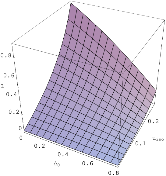
FIG. 1.: Variation of the function $L\left(u_{iso},\Delta_{0}\right)$ against the anisotropy parameter $\Delta_{0}$ and $u_{iso}$.

Generally, the condition (29) is satisfied for $0\leq\Delta_{0}<1$ and $u_{iso}\leq 0.3$.

III Astrophysical Applications

When the thermonuclear sources of energy in its interior are exhausted, a spherical star begins to collapse under the influence of gravitational interaction of its matter content. The mass energy continues to increase and the star ends up as a compact relativistic cosmic object such as neutron star, strange star or black hole. Important observational quantities for such objects are the surface redshift, the central redshift and the mass and radius of the star.

For a relativistic anisotropic star described by the solution presented in the previous Section the surface redshift $z_{s}$ is given by

$$z_{s}=\left(1-\frac{4}{2+\Delta_{0}}u_{iso}\right)^{-1/2}-1.$$ (30)

The surface redshift is decreasing with increasing $\Delta_{0}$. Hence, at least in principle, the study of redshift of light emitted at the surface of compact objects can lead to the possibility of observational detection of anisotropies in the internal pressure distribution of relativistic stars. Using the density variation parameter $\mu=\rho(R)/\rho(0)$, Patel and Mehra [29] discussed numerical estimates of various physical parameters in their model and concluded that the surface redshift in the isotropic case is greater than the surface redshift in the anisotropic case. Hence, our results are very similar to that of [29].

The central redshift $z_{c}$ is of the form

$$z_{c}=\alpha_{1}^{-1/2}\left[1+\beta_{1}\left(5-2\Delta_{0}\right)\sqrt{2+\Delta_{0}}\right]^{-1}-1.$$ (31)

The variation of the central redshift of the neutron star against the anisotropy parameter is represented in Fig. 2.

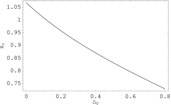
FIG. 2.: Variation of the central redshift $z_{c}$ as a function of the anisotropy parameter $\Delta_{0}$ for a static anisotropic fluid sphere with $u_{iso}=0.27$.

Clearly, in our model the anisotropy introduced in the pressure gives rise to a decrease in the central redshift. Hence, as functions of the anisotropy, the central and surface redshifts have the same behavior.

The stellar model presented here can be used to describe the interior structure of the realistic neutron star. Taking the surface density of the star as $\rho_{s}=2\times 10^{14}g/cm^{3}$ and with the use of Eqs. (17) we obtain

$$\rho_{s}R_{N}^{2}=\frac{3X\left(3+X\right)}{\left(2+\Delta_{0}\right)\left(1+X\right)^{2}},$$ (32)

or

$$R_{N}=18.891u_{iso}^{1/2}\left(9-8u_{iso}\right)^{1/2}\left(2+\Delta_{0}\right)^{-1/2}km,$$ (33)

where $R_{N}$ is the radius of the neutron star corresponding to a specific surface density. For the mass $M_{N}$ and anisotropy parameter $\Delta_{N}$ we find

$$M_{N}=25.568u_{iso}^{3/2}\left(9-8u_{iso}\right)^{1/2}\left(2+\Delta_{0}\right)^{-3/2}M_{\odot},$$ (34)

$$\Delta_{N}=7.19004\times 10^{35}\Delta_{0}u_{iso}\left(9-8u_{iso}\right)^{-1}dyne{\ }cm^{-2}.$$ (35)

With $\Delta_{0}=0$ we recover the results for $\left(M_{N},R_{N}\right)$ given by Durgapal and Bannerji [25]. In Eqs. (33)-(35), for the sake of simplicity, we have expressed all the quantities in international units, instead of natural units, by means of the transformations $\frac{M_{N}}{R_{N}}\rightarrow 8\pi\frac{GM_{N}}{c^{2}R_{N}}$, $\rho\rightarrow\rho c^{2}$ and $\Delta_{N}\rightarrow\frac{8\pi G}{c^{4}}\Delta_{N}$, where $G=6.6732\times 10^{-8}dyne{\ }cm^{2}{\ }g^{-2}$ and $c=2.997925\times 10^{10}cm{\ }s^{-1}$.

The variation of the anisotropy parameter $\Delta_{N}$ of the neutron star as a function of the radius $R_{N}$ and mass $M_{N}$ is represented in Fig. 3.

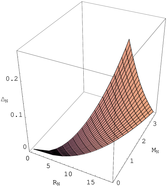
FIG. 3.: Variation of the anisotropy parameter $\Delta_{N}$ (in units of $10^{35}dynecm^{-2}$) of the neutron star as a function of the radius $R_{N}(km)$ and mass $M_{N}$ (in solar mass units) for $\Delta_{0}\in\left[0,0.9\right]$ and $u_{iso}\in\left[0.0001,0.28\right]$ .

For a particular choice of the equation of state at the center of the star, $3p_{r0}=3p_{\perp 0}=\rho_{0}$ and with a vanishing anisotropy parameter, $\Delta_{0}=0$, we obtain the result $u_{iso}=0.2908526$ for a static isotropic fluid sphere that can be compared with the value of $u_{iso}$ given in [25].

The quantities $\left(\frac{dp_{r}}{d\rho}\right)_{r=0}$, $\left(\frac{dp_{\perp}}{d\rho}\right)_{r=0}$ , $\left(\frac{dp_{r}}{d\rho}\right)_{r=R}$ and $\left(\frac{dp_{\perp}}{d\rho}\right)_{r=R}$ are represented against the anisotropy parameter $\Delta_{0}$ in Fig. 4.

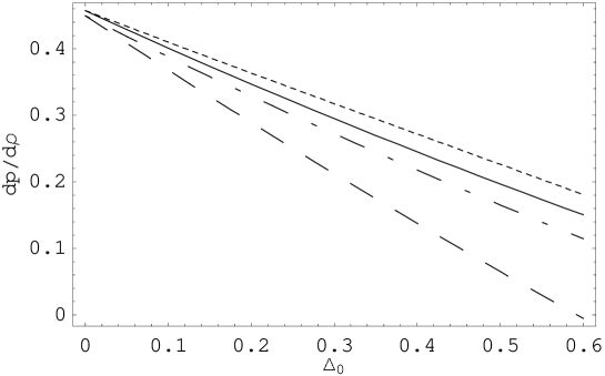
FIG. 4.: Variations of the radial and tangential speeds of sound $dp/d\rho$ at the vacuum boundary and at the center of the anisotropic fluid sphere as a function of the anisotropy parameter $\Delta_{0}$ for $u_{iso}=0.24$: $\left(dp_{r}/d\rho\right)_{r=R}$ (dotted curve); $\left(dp_{\perp}/d\rho\right)_{r=R}$ (full curve); $\left(dp_{r}/d\rho\right)_{r=0}$ (dashed-dotted curve); $\left(dp_{\perp}/d\rho\right)_{r=0}$ (dashed curve).

The plots indicate that the necessary and sufficient criterion for the adiabatic speed of sound to be less than the speed of light is satisfied by our solution. However, Caporaso and Brecher [26] claimed that $dp/d\rho$ does not represent the signal speed. If therefore this speed exceeds the speed of light, this does not necessary mean that the fluid is non-causal. But this argument is quite controversial and not all authors accept it [27].

IV Discussions and Final Remarks

Curvature is described by the tensor field $R_{ijk}^{l}$. It is well known that if one uses singular behavior of the components of this tensor or its derivatives as a criterion for singularities, one gets into trouble since the singular behavior of components could be due to singular behavior of the coordinates or tetrad basis rather than that of the curvature itself. To avoid this problem, one should examine the linear and quadratic scalars formed out of curvature, such as $r_{1}=R$, $r_{2}=R_{ij}R^{ij}$ and $r_{3}=R_{ijkl}R^{ijkl}$.

With the use of the gravitational field equations (7)- (8) and of the static line element (4) we obtain the following expressions for the linear and quadratic scalars of the curvature tensor, given in terms of the radial pressure, energy density, mass and anisotropy parameter:

$$r_{1}=3p_{r}-\rho+2\Delta,$$ (36)

$$r_{2}=\rho^{2}+3p_{r}^{2}+2\Delta\left(\Delta+2p_{r}\right),$$ (37)

$$r_{3}=\left(2\Delta+\rho+p_{r}-\frac{4m}{r^{3}}\right)^{2}+2\left(p_{r}+\frac{2m}{r^{3}}\right)^{2}+2\left(\rho-\frac{2m}{r^{3}}\right)^{2}+4\left(\frac{2m}{r^{3}}\right)^{2}.$$ (38)

When $\Delta=\rho=p_{r}=0$, we recover the invariant $R_{ijkl}R^{ijkl}$ for the Schwarzschild line element, that is $r_{3}=48m^{2}/r^{6}$. The variations of $r_{1}$, $r_{2}$ and $r_{3}$ are represented in Fig. 5.

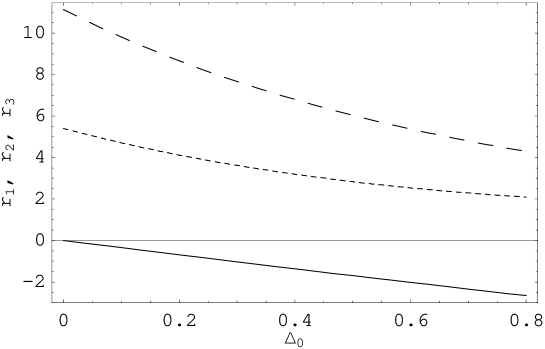
FIG. 5.: Variation of the curvature scalar $r_{1}$ (solid curve) and of the linear and quadratic scalars of the curvature tensor $r_{2}$ (dotted curve) and $r_{3}$ (dashed curve) of the static anisotropic fluid sphere against the anisotropy parameter $\Delta_{0}$ for $u_{iso}=0.2908526$.

The scalars $r_{2}$ and $r_{3}$ are finite at the center of the fluid sphere and monotonically decrease as the anisotropy parameter $\Delta_{0}$ increases.

It is generally held that the trace $T$ of the energy-momentum tensor must be non-negative. It is also the case that this trace condition is everywhere fulfilled if it is fulfilled at the center of the star [28].

The purpose of the present paper is to present some exact models of static anisotropic fluid stars and to investigate their possible astrophysical relevance. We have extended and generalized to the anisotropic case the method of obtaining exact solutions for relativistic spheres of Buchdahl [24] and Durgapal and Bannerji [25]. All the solutions we have obtained are non-singular inside the anisotropic sphere, with finite values of the density and pressure at the center of the star. Variations of the physical parameters mass, radius, redshift and adiabatic speed of sound against the anisotropy parameter have been presented graphically. Our model can be used to study the interior structure of the anisotropic relativistic objects because it satisfies all the physical conditions and requirements (a)-(f).

REFERENCES

- [1] R. L. Bowers, E. P. T. Liang, Astrophys. J. 188 (1974) 657
- [2] R. Ruderman, Ann. Rev. Astron. Astrophys. 10 (1972) 427
- [3] R. Kippenhahm, A. Weigert, Stellar Structure and Evolution, Springer, Berlin 1990
- [4] A. I. Sokolov, JETP 52 (1980) 575
- [5] R. F. Sawyer, Phys. Rev. Lett. 29 (1972) 382
- [6] J. Binney, S. Tremaine, Galactic Dynamics, Princeton University Press, Princeton, New Jersey 1987
- [7] L. Herrera, N. O. Santos, Astrophys. J. 438 (1995) 308
- [8] P. Letelier, Phys. Rev. D 22 (1980) 807
- [9] S. S. Bayin, Phys. Rev. D 26 (1982) 1262
- [10] H. Heintzmann, W. Hillebrandt, Astron. Astrophys. 38 (1975) 51
- [11] W. Hillebrandt, K. O. Steinmetz, Astron. Astrophys. 53 (1976) 283
- [12] M. Cosenza, L. Herrera, M. Esculpi, L. Witten, J. Math. Phys. 22 (1981) 118
- [13] K. D. Krori, P. Bargohain, R. Devi, Can. J. Phys. 62 (1984) 239
- [14] S. D. Maharaj, R. Maartens, Gen. Rel. Grav. 21 (1989) 899
- [15] B. W. Stewart, J. Phys. A: Math. Gen. 15 (1982) 2419
- [16] T. Singh, G. P. Singh, R. S. Srivastava, Int. J. Theor. Phys. 31 (1992) 545
- [17] G. Magli, J. Kijowski, Gen. Rel. Grav. 24 (1992) 139
- [18] G. Magli, Gen. Rel. Grav. 25 (1993) 441
- [19] T. Harko, M. K. Mak, J. Math. Phys. 41 (2000) 4752
- [20] H. Bondi, Month. Not. R. Acad. Sci. 259 (1992) 365
- [21] R. Chan, L. Herrera, N. O. Santos, Month. Not. R. Acad. Sci. 265 (1993) 533
- [22] L. Herrera, J. Ponce de Leon, J. Math. Phys. 26 (1985) 2302
- [23] M. K. Gokhroo, A. L. Mehra, Gen. Rel. Grav. 26 (1994) 75
- [24] H. A. Buchdahl, Phys. Rev. 116 (1959) 1027
- [25] M. C. Durgapal, R. Bannerji, Phys. Rev. D 25 (1983) 328
- [26] G. Caporaso, K. Brecher, Phys. Rev. D 20 (1979) 1823
- [27] E. N. Glass, Phys. Rev. D 28 (1983) 2693
- [28] H. Knutsen, Month. Not. R. Acad. Sci. 232 (1988) 163
- [29] L. K. Patel, N. P. Mehra, Aust. J. Phys. 48 (1995) 635
- [30] M. S. R. Delgaty, K. Lake, Comput. Phys. Commun. 115 (1998) 395
- [31] L. Herrera, N. O. Santos, Phys. Reports 286 (1997) 53