A survey of spinning test particle orbits in Kerr spacetime

Abstract

We investigate the dynamics of the Papapetrou equations in Kerr spacetime. These equations provide a model for the motion of a relativistic spinning test particle orbiting a rotating (Kerr) black hole. We perform a thorough parameter space search for signs of chaotic dynamics by calculating the Lyapunov exponents for a large variety of initial conditions. We find that the Papapetrou equations admit many chaotic solutions, with the strongest chaos occurring in the case of eccentric orbits with pericenters close to the limit of stability against plunge into a maximally spinning Kerr black hole. Despite the presence of these chaotic solutions, we show that physically realistic solutions to the Papapetrou equations are not chaotic; in all cases, the chaotic solutions either do not correspond to realistic astrophysical systems, or involve a breakdown of the test-particle approximation leading to the Papapetrou equations (or both). As a result, the gravitational radiation from bodies spiraling into much more massive black holes (as detectable, for example, by LISA, the Laser Interferometer Space Antenna) should not exhibit any signs of chaos.

I INTRODUCTION

The present paper continues the investigation initiated in Hartl (2003), which considered the dynamics of spinning test particles (i.e., compact astrophysical objects) orbiting a spinning black hole (Kerr spacetime). The primary objective is to determine whether the orbits of spinning compact objects spiraling into much more massive black holes are chaotic or not. Evidence for chaotic orbits in relativistic binaries has been presented in Suzuki and Maeda (1997); Levin (2000, ); Cornish (2001); Cornish and Levin (2002, ) (although only Suzuki and Maeda (1997) was directly concerned with the extreme mass ratio systems we consider here). An astrophysical example of the systems we consider is a solar-mass black hole or neutron star orbiting a supermassive black hole in a galactic nucleus. Such systems are potentially important sources of gravitational radiation in frequency bands detectable by space-based gravitational wave detectors such as the proposed Laser Interferometer Space Antenna (LISA) mission. The methods of data analysis for signals from such detectors typically rely on matched filters, which use a discrete mesh in parameter space to achieve a given signal-to-noise ratio. The presence of chaos would cause the number of templates needed to fit a given signal to grow exponentially with decreasing mesh size, potentially overwhelming the computers performing the analysis.

Many studies have used the Papapetrou equations to investigate the dynamics of spinning test particles in the background spacetime of a central black hole (including most recently Tanaka et al. (1996); Suzuki and Maeda (1997); Hartl (2003); Semerák (1999); Suzuki and Maeda (2000); see Semerák (1999) and Suzuki and Maeda (2000) for a more thorough literature review). We found in Hartl (2003) that the Papapetrou equations formally admit chaotic solutions in Kerr spacetime, but the chaos seemed to disappear for physically realistic spins. This conclusion was tentative, since we investigated only a few values of the many parameters appearing in the equations. In the present study, we undertake a thorough search of parameter space in order to determine the prevalence of chaotic orbits, both for dynamically interesting (but physically unrealistic) orbits with high spin parameter $S$ and for astrophysically relevant systems with smaller spin.

As in Hartl (2003), we use Lyapunov exponents to measure the divergence of nearby trajectories and to provide an estimate for the timescale of the divergence. For chaotic systems, initial conditions separated by a small distance $\epsilon_{0}$ diverge exponentially, with the separation growing as $\epsilon(\tau)=\epsilon_{0}\,e^{\lambda\tau}$, where $\lambda$ is the Lyapunov exponent. For nonchaotic orbits, $\lambda=0$, but when $\lambda$ is nonzero it provides the $e$-folding timescale $\tau_{\lambda}=1/\lambda$ for chaotic behavior to manifest itself. In this paper we use two rigorous methods for determining the maximum Lyapunov exponent $\lambda_{\mathrm{max}}$ described in Hartl (2003). Further details appear below in Sec. IV and in Sec. III of Hartl (2003).

Our parameter space search makes use of a convenient orbital parameterization technique, which allows us to specify desired values of pericenter $r_{p}$ and orbital inclination $\iota$ (Sec. III). We vary these orbital parameters along with spin magnitude, eccentricity, Kerr spin angular momentum $a$, and spin inclination, and calculate the largest Lyapunov exponent for each set of initial conditions. A complete description of our methods for searching parameter space appears in Sec. V. Though not exhaustive, the resulting survey of parameter space gives a thorough picture of chaos in the Papapetrou equations with a Kerr background.

We set $G=c=1$, use sign conventions as in MTW (Misner et al., 1973), and use Boyer-Lindquist coordinates $(r,\theta,\phi)$ for Kerr spacetime. We use vector arrows for 4-vectors and boldface for Euclidean vectors. The symbol $\log$ denotes the natural logarithm.

II Spinning test particles

We use the Papapetrou equations of motion (Papapetrou, 1951) to model a spinning test particle. As reformulated by Dixon (Dixon, 1970), these equations describe the motion of a “pole-dipole particle,” which neglects effects smaller than those due to the mass monopole and spin dipole (thus neglecting the tidal coupling, which is a mass quadrupole effect). The Papapetrou equations describe a particle with negligible mass compared to the masses responsible for generating the background spacetime. In our case, we write $\mu$ for the test particle’s mass and $M$ for the mass of the central Kerr black hole; the test particle limit then requires that $\mu\ll M$.

II.1 Equations of motion

Dixon’s formulation for the equations of motion uses an antisymmetric spin tensor $S^{\mu\nu}$ to represent the spin angular momentum of the particle. The covariant derivative of the 4-momentum $p^{\mu}$ deviates from the nonspinning (geodesic) case by a term representing a coupling of the spin to the background spacetime curvature. If we write $v^{\mu}$ for the 4-velocity, the full equations of motion appear as follows:

$$\frac{dx^{\mu}}{d\tau} = v^{\mu}$$

$$\nabla_{\vec{v}}\,p^{\mu} = -\textstyle{\frac{1}{2}}R^{\mu}_{\ \nu\alpha\beta}\,v^{\nu}S^{\alpha\beta}$$ (1)

$$\nabla_{\vec{v}}\,S^{\mu\nu} = 2p^{[\mu}v^{\nu]}.$$

Here $R^{\mu}_{\ \nu\alpha\beta}$ is the Riemann curvature tensor of the spacetime, which in our case corresponds to the Riemann tensor for the Kerr metric. Note that in the case of vanishing spin (all components of $S^{\mu\nu}$ equal to zero) or flat spacetime (all components of $R^{\mu}_{\ \nu\alpha\beta}$ equal to zero), we recover the geodesic equation $\nabla_{\vec{v}}\,p^{\mu}=0$.

For numerical and conceptual purposes, we use a reformulation of the equations of motion in terms of the momentum 1-form $p_{\mu}$ and spin 1-form $S_{\mu}$. The spin 1-form can be derived from the 4-momentum and spin tensor using

$$S_{\mu}=\textstyle{\frac{1}{2}}\epsilon_{\mu\nu\alpha\beta}\,u^{\nu}S^{\alpha\beta},$$ (2)

where $u^{\nu}=p^{\nu}/\mu$. The spin 1-form is easier to visualize than the spin tensor, and the Papapetrou equations are better-behaved numerically in the $S\rightarrow 0$ limit when expressed in terms of the spin 1-form. Details of this formulation appear in Hartl (2003) and the appendix.

II.2 General constraints

The Papapetrou system of equations (II.1) is highly constrained, even in arbitrary spacetimes. The 4-momentum and spin satisfy normalization conditions that are conserved by the equations of motion:

$$p^{\mu}p_{\mu}=-\mu^{2}$$ (3)

and

$$\textstyle{\frac{1}{2}}S^{\mu\nu}S_{\mu\nu}=S^{2}.$$ (4)

A further condition is required to identify a unique worldline for the center of mass:

$$p_{\mu}S^{\mu\nu}=0.$$ (5)

A more detailed discussion of this “spin supplementary condition” appears in Hartl (2003).

II.3 Kerr constraints

The Papapetrou equations share an important property with geodesic motion, namely, to each symmetry of the background spacetime (typically represented by a Killing vector) there corresponds a constant of the motion. Kerr spacetime has two such symmetries, which provide two constraints in addition to those described in the previous section. (The Killing tensor that leads to the Carter constant in the geodesic does not correspond to a conserved quantity when the spin is nonzero; see Sec. III.2.3 below.)

For each Killing vector $\vec{\xi}$ there corresponds a constant given by the standard expression for geodesics plus a contribution due to a coupling with the spin tensor:

$$C_{\xi}=\xi^{\mu}p_{\mu}-\textstyle{1\over 2}\xi_{\mu;\nu}S^{\mu\nu}.$$ (6)

Kerr spacetime’s two Killing vectors $\vec{\xi}^{t}=\partial/\partial t$ and $\vec{\xi}^{\phi}=\partial/\partial\phi$ then give energy and $z$ angular momentum conservation:

$$-E=p_{t}-\textstyle{1\over 2}g_{t\mu,\nu}S^{\mu\nu}$$ (7)

and

$$J_{z}=p_{\phi}-\textstyle{1\over 2}g_{\phi\mu,\nu}S^{\mu\nu}.$$ (8)

II.4 The spin parameter $S$

The spin magnitude $S$ that appears in Eq. (4) quantifies the size of the spin and thus plays a crucial role in determining the behavior of spinning test particle systems. As in Hartl (2003), we measure distances and times in terms of $M$ and momenta in terms of $\mu$. In these units, $S$ is measured in units of $\mu M$. When measured in traditional geometrized units, the spin of a black hole can be as large as its mass squared, i.e., $S_{\mathrm{geom,\,max}}=\mu^{2}$. In this case the spin parameter goes like $S\sim\mu^{2}/(\mu M)=\mu/M$, which is necessarily small for a test particle system. This result applies to all astrophysically relevant systems, as shown in Hartl (2003). Thus, we have the important physical constraint that the spin parameter $S$ must satisfy $S\ll 1$ for all physically realistic systems. A thorough discussion of various possibilities (including neutron stars and white dwarfs) in Hartl (2003) showed that realistic values of $S$ for LISA sources fall in the range $10^{-4}$–$10^{-7}$.

The smallness of the spin’s effect is not dependent on our choice to measure $S$ in terms of $\mu M$. If instead we measure $S$ in terms of $\mu^{2}$, then the equation of motion for $S^{\mu\nu}$ becomes (rewriting $\nabla_{\vec{v}}$ as $D/d\tau$)

$$\frac{D(S^{\mu\nu}/\mu^{2})}{d(\tau/M)}=2\,\frac{1}{\mu}p^{[\mu}v^{\nu]},$$ (9)

where we have factored out from each variable its corresponding scale factor. This gives

$$\frac{DS^{\mu\nu}}{d\tau}=\frac{\mu}{M}\left(2p^{[\mu}v^{\nu]}\right),$$ (10)

so that in these units the spin’s effective magnitude is suppressed by a factor of $\mu/M$. Measuring $S$ in terms of $\mu M$ effectively absorbs the unavoidable smallness of the spin effect into the spin parameter itself.

III Parameterizing initial conditions

The many constraints on the equations of motion lead to considerable complexity in parameterizing the initial conditions. We summarize here the primary parameterization method described in Hartl (2003), and then discuss in detail a method for parameterizing initial conditions using the geometrical properties of the orbit.

III.1 Energy and angular momentum parameterization

It is easy to parameterize the Papapetrou equations directly in terms of the momentum and spin components, but more physically relevant parameterizations are more difficult. The parameterization method discussed in Hartl (2003) solves for the initial conditions using the integrals of the motion $E$ and $J_{z}$. This method also serves as the foundation for a more sophisticated parameterization in terms of orbital parameters (Sec. III.2).

The energy and angular momentum parameterization method proceeds as follows. If we think of the system in terms of the spin 1-form $S_{\mu}$, we have twelve variables, four each for position, 4-momentum, and spin. Since Kerr spacetime is static and axially symmetric, without loss of generality we may set the initial time and axial angle to zero: $\tau=\phi=0$. (We use the proper time $\tau$ as our time parameter, as discussed in Sec. IV below.) We then provide the initial values for $r$, $\theta$, and $p_{r}$, together with the constants $E$, $J_{z}$, and $S$. Finally, we provide two components of the spin vector in an orthonormal basis. It is easiest to specify the radial and $\theta$ components $S^{\hat{r}}$ and $S^{\hat{\theta}}$; since the $r$-$\theta$ part of the Kerr metric is diagonal, we may then easily derive the 1-form components $S_{r}$ and $S_{\theta}$.

Having specified values for seven of the variables, we must now use the five equations that relate them. Since we measure the particle’s momentum in terms of its rest mass $\mu$, the momentum normalization relation is

$$p^{\mu}p_{\mu}=-1,$$ (11)

which we use to eliminate $p_{\theta}$. We then solve the spin normalization condition

$$S^{\mu}S_{\mu}=S^{2}$$ (12)

to eliminate $S_{\phi}$. The spin-momentum orthogonality constraint and the two integrals of the motion then give three equations in the three remaining unknowns $p_{t}$, $p_{\phi}$, and $S_{t}$:

$$0 = p_{\mu}S_{\nu}g^{\mu\nu}$$ (13)

$$E = -p_{t}+\textstyle{1\over 2}g_{t\mu,\nu}S^{\mu\nu}$$ (14)

$$J_{z} = p_{\phi}-\textstyle{1\over 2}g_{\phi\mu,\nu}S^{\mu\nu}$$ (15)

(The first of these equations is equivalent to the condition $p_{\mu}S^{\mu\nu}=0$, as discussed in the appendix.)

We solve Eqs. (13)–(15) with a Newton-Raphson root finder, which works robustly given good initial guesses. The terms $\textstyle{1\over 2}g_{t\mu,\nu}S^{\mu\nu}$ and $\textstyle{1\over 2}g_{\phi\mu,\nu}S^{\mu\nu}$ are typically small, even in the physically unrealistic case of $S\sim 1$, so $E$ and $J_{z}$ are good initial guesses for their corresponding momenta. We typically use $S_{\theta}$ as the initial guess for $S_{t}$. In all cases, we verify a posteriori that all constraints are satisfied to within machine precision.

III.2 Orbital geometry parameterization

While the method described above is sufficient for determining a set of valid initial conditions, parameterizing orbits by energy and angular momentum is not particularly intuitive. It is much more natural to think in terms of the orbital geometry, so we prefer to parameterize by the pericenter $r_{p}$, the eccentricity $e$, and the orbital inclination angle $\iota$. Such parameters only have precise meaning for geodesic orbits, but are nevertheless still useful for the case of spinning test particles.

III.2.1 Kerr geodesics

The first step in parameterizing solutions of the Papapetrou-Dixon equations using orbital parameters is to solve the geodesic case. The traditional method for specifying a geodesic in terms of conserved quantities uses the energy $E$, the $z$ angular momentum $L_{z}$, and the Carter constant $Q$ Misner et al. (1973). In order to use the orbital parameters, we adopt a mapping from $(r_{p},e,\iota)$ to $(E,L_{z},Q)$ based on unpublished notes supplied by Teviet Creighton and Scott Hughes (and implemented in Hughes’s Kerr geodesic integrator Hughes ).

In order to use the more intuitive orbital parameters, we must determine the set $(E,L_{z},Q)$ given the set $(r_{p},e,\iota)$. We obtain two of the necessary equations by noting that the radial velocity $dr/d\tau$ vanishes at pericenter and apocenter, since these radii correspond to turning points in the radial motion. The equation for the time-evolution of the Boyer-Lindquist radius $r$ is Misner et al. (1973):

$$\Sigma^{2}\left(\frac{dr}{d\tau}\right)^{2}=R(r),$$ (16)

where

$$R(r)=[E(r^{2}+a^{2})-aL_{z}]^{2}-\Delta[r^{2}+(L_{z}-aE)^{2}+Q],$$ (17)

and we use the standard auxiliary variables

$$\Sigma=r^{2}+a^{2}\cos^{2}\theta$$ (18)

and

$$\Delta=r^{2}-2Mr+a^{2}.$$ (19)

The quantity $a$ is the Kerr spin parameter $J/M$, i.e., the central black hole’s spin angular momentum per unit mass, which is dimensionless in our normalized units. From Eq. (17) we see that $dr/d\tau=0$ implies that $R(r)=0$, so we obtain one equation at each turning point:

$$R(r_{p})=0$$ (20)

and

$$R(r_{a})=0,$$ (21)

where the apocenter is defined by

$$r_{a}=\left(\frac{1+e}{1-e}\right)\,r_{p}.$$ (22)

The final equation required to complete the mapping is Ryan (1996)

$$Q=L_{z}^{2}\,\tan^{2}\iota.$$ (23)

The value of $\iota$ resulting from this definition agrees closely with the maximum value of $|\pi/2-\theta|$ for a numerically determined solution to the equations of motion, i.e., it faithfully captures a geometric property of the orbit.

Eqs. (20)–(23) give three equations in three unknowns, which are easy to solve using a nonlinear root finder as long as good initial guesses for the energy, angular momentum, and Carter constant can be found. The approach we adopt uses the degenerate cases of circular equatorial orbits to provide the raw material for analytical guesses. The energies for prograde and retrograde circular orbits in the equatorial plane are

$$E^{\mathrm{pro}}(r)=\frac{1-2v^{2}+\tilde{a}v^{3}}{\sqrt{1-3v^{2}+2\tilde{a}v^{3}}}$$ (24)

and

$$E^{\mathrm{ret}}(r)=\frac{1-2v^{2}-\tilde{a}v^{3}}{\sqrt{1-3v^{2}-2\tilde{a}v^{3}}},$$ (25)

where we write $v\equiv\sqrt{M/r}$ and $\tilde{a}=a/M$ for notational simplicity. The initial guess for the energy is then an average of these energies, weighted using the inclination angle, with “radius” given by the semimajor axis of an ellipse with pericenter $r_{p}$ and eccentricity $e$:

$$E^{\mathrm{guess}}=\textstyle{\frac{1}{2}}\left[\alpha_{+}\,E^{\mathrm{pro}}(r_{\mathrm{semi}})+\alpha_{-}\,E^{\mathrm{ret}}(r_{\mathrm{semi}})\right],$$ (26)

where

$$\alpha_{\pm}=1\pm\cos\iota,$$ (27)

and

$$r_{\mathrm{semi}}=\frac{r_{p}}{1-e}.$$ (28)

It is possible (though rare) for Eq. (26) to yield an energy guess greater than 1; in this case, we simply set $E^{\mathrm{guess}}=1$.

Once we have a guess for the energy, we can find the corresponding guess for the angular momentum. Using the value from Eq. (26) and the expression for the angular momentum for a circular equatorial orbit gives

$$L_{z}^{\mathrm{guess}}=\cos\iota\,\sqrt{\frac{1-e^{2}}{2(1-E^{\mathrm{guess}})}}$$ (29)

as an initial guess for the angular momentum. Finally, the guess for the Carter constant is

$$Q^{\mathrm{guess}}=\left(L_{z}^{\mathrm{guess}}\right)^{2}\,\tan^{2}\iota.$$ (30)

Plugging Eqs. (26), (29), and (30) into the nonlinear root finder yields the actual values of $E$, $L_{z}$, and $Q$ to within machine precision in fewer than 10 iterations.

One caveat about our parameterization method is worth mentioning: some values of $(r_{p},e,\iota)$ correspond to unstable Kerr orbits, and in this case the method returns a set $(E,L_{z},Q)$ corresponding to an orbit with a different pericenter from the one requested. We can illustrate this behavior by factoring Eq. (17), which is a quartic function in $r$:

$$R(r)=(1-E^{2})(r_{1}-r)(r-r_{2})(r-r_{3})(r-r_{4}).$$ (31)

The roots are ordered so that $r_{1}\geq r_{2}\geq r_{3}\geq r_{4}$. Bound motion occurs for $r_{1}\geq r\geq r_{2}$, which implies that $r_{1}=r_{a}$ and $r_{2}=r_{p}$, but this only works for stable orbits. In the case that the orbit requested is unstable, the set $(r_{p},e,\iota)$ returned by the algorithm instead corresponds to a nearby, stable orbit. In this case, the numerically calculated roots of $R(r)$ satisfy $r_{3}=r_{p,\,\mathrm{requested}}$, but the parameterization method returns $r_{2}$ as the pericenter, i.e., it returns a nearby stable orbit with pericenter $r_{p}=r_{2}>r_{p,\,\mathrm{requested}}$. As a result, the actual pericenter is larger than the value requested.

We use routines from Hughes to identify the boundary between stable and unstable orbits (so that the latter may be excluded), but the code has a few minor bugs, and the identification procedure is not infallible. As a result, some such orbits appear in the results below (Sec. V) and can be identified by having pericenters different from those requested. It is essential to understand, however, that the orbits returned by the parameterization algorithm are never unstable, and represent perfectly valid (stable) solutions to the equations of motion.

III.2.2 From Kerr geodesics to Papapetrou initial conditions

Once we have the set $(E,L_{z},Q)$ for the geodesic case, we can use the well-known properties of the Kerr metric to solve for all the parameters necessary for the method described in Sec. III.1 above. The first step is to force the constants of the motion to agree by setting $E_{\mathrm{Papapetrou}}=E_{\mathrm{Kerr}}$ and $J_{z}=L_{z}$. Next, we set $\theta_{0}=\pi/2$ (corresponding to the equatorial plane), since this is the only angle guaranteed to be shared by all Kerr geodesic orbits. Finally, we must choose an initial value $r_{0}$ for the Boyer-Lindquist radius, which in the case of $\theta_{0}=\pi/2$ coincides with the crossing of the equatorial plane. One possibility is simply to use the average value of the pericenter and apocenter,

$$r_{0}=\textstyle{\frac{1}{2}}(r_{p}+r_{a}).$$ (32)

This radius is guaranteed to lie between pericenter and apocenter, and the prescription in Eq. (32) works fine for the mildly eccentric orbits considered in this paper, but a more robust method must take into account that highly eccentric orbits should in general cross the equatorial plane near pericenter. (Requiring a plane-crossing far from pericenter would force the inclination angle to be small, which is a constraint we do not wish to impose.) This suggests choosing an initial value of $r$ close to pericenter. One flexible method is to choose

$$r_{0}=r_{p}(1+\alpha e),$$ (33)

where $\alpha$ is a number of order unity. This reduces correctly to $r_{p}$ in the $e=0$ (circular) limit, and selects an equatorial plane crossing near pericenter in the $e\sim 1$ limit. If we set $\alpha=2$ in Eq. (33), then this method agrees exactly with Eq. (32) in the cases $e=0$ and $e=0.5$, and differs from Eq. (32) by less than 15% when $e=0.6$. Most of the results in this paper use Eq. (32), but Eq. (33) is preferable in general.

Once the initial $\theta$ and $r$ are known, we can determine all components of the Kerr 4-momentum $p_{K}^{\mu}$, but three of the Papapetrou momenta are determined by the constraints (Sec. III.1). We are therefore free to force only one of the four components of the Papapetrou momentum $p_{P}^{\mu}$ to be the same as its Kerr counterpart. For the bulk of this paper, we set the radial components equal ($p_{K}^{r}=p_{P}^{r}$), since it is the radial momentum that is most closely tied to the stability and boundedness of the orbits. This choice results in Papapetrou orbits with pericenters and eccentricities fairly close to the Kerr geodesic values, but with much higher orbital inclination angles (Fig. 7). The alternate choice of $p_{K}^{\theta}=p_{P}^{\theta}$ results in Papapetrou orbits with inclinations similar to their Kerr counterparts, but with very different pericenters (Fig. 8). See Sec. V for further discussion.

We determine a value for the radial Papapetrou momentum $p_{P}^{r}$ using the Kerr geodesic parameters $E_{K}$, $L_{z}$, and $Q$ by applying Eq. (17) and the equation

$$\rho^{2}p^{r}=\mu\sqrt{R(r)},$$ (34)

where $\rho=r^{2}+a^{2}\cos^{2}\theta$ Misner et al. (1973). We then convert to $p_{r}$ using $p_{r}=p^{r}g_{rr}$. Proceeding exactly as in Sec. III.1, we specify two of the spin components and eliminate two variables using 4-momentum and spin normalization, and then solve numerically for $p_{t}$, $p_{\phi}$, and $S_{t}$. The result is a set of initial conditions for the Papapetrou equations with the same energy and angular momentum as a Kerr geodesic with the desired values of $r_{p}$, $e$, and $\iota$.

It sometimes happens that the Papapetrou initial conditions derived in this manner specify an orbit that is unstable against plunge into the black hole. Since there is no “effective potential” for a generic Papapetrou orbit as there is for Kerr geodesics, there is no way a priori to detect this instability. Plunge orbits are detected at runtime by testing for radial coordinates less than the horizon radius. Orbits that plunge are removed from consideration since by definition they cannot be chaotic.

III.2.3 Empirical orbital parameters

In making the transition from geodesics to solutions of the Papapetrou equations, we are able to enforce the conditions $E_{\mathrm{Papapetrou}}=E_{\mathrm{Kerr}}$ and $J_{z}=L_{z}$, but this is no guarantee that the Papapetrou orbit has the corresponding orbital parameters $r_{p}$ and $\iota$: the spin-coupling term $-\frac{1}{2}\xi_{\mu;\nu}S^{\mu\nu}$ [cf. Eq. (6)] has a potentially large effect on the empirical values of the pericenter and orbital inclination. This effect is most pronounced when we consider high spin parameter values, i.e., $S\sim 1$. In these dynamically interesting cases, the empirical pericenter and inclination will differ in general from the values requested in the parameterization.

The empirical Papapetrou pericenter $r_{p,\,P}$ is easy to find: we simply integrate the orbit with a small stepsize for a large number of periods, and then record the minimum radius achieved. In practice, this works robustly, reproducing almost exactly the requested Kerr value of $r_{p,\,K}$ in the limit $S\ll 1$. The only exception involves values of $r_{p,\,K}$ that correspond to requested unstable orbits, as discussed in Sec. III.2.1 above. Each of these orbits has an empirical pericenter larger than the pericenter requested: the requested pericenter corresponds to the root $r_{3}$ in Eq. (31), but the empirical pericenter returned by the algorithm corresponds to the larger root $r_{2}$.

Having found the empirical pericenter for an orbit, we must next find its empirical orbital inclination angle $\iota_{P}$. In order to reproduce the definition from Eq. (23), we need to find an analogue of the Carter constant $Q$ for spinning test particles. Kerr spacetime has a Killing tensor $K_{\mu\nu}$ Wald (1984) that satisfies

$$K_{\mu(\nu;\alpha)}=0,$$ (35)

which gives rise to an extra conserved quantity in the case of geodesic motion:

$$K=K_{\mu\nu}p^{\mu}p^{\nu}.$$ (36)

This quantity is related to the traditional Carter constant $Q$ by Misner et al. (1973)

$$K=Q+(L_{z}-aE)^{2}.$$ (37)

When the test particle has nonzero spin, the quantity defined by Eq. (37) is no longer constant, but there is an analogous expression that is conserved to linear order. Adapting a result from Tanaka et al. (1996), we can write this approximately conserved quantity as

$$C=K_{\mu\nu}p^{\mu}p^{\nu}-2p^{\mu}S^{\rho\sigma}(f^{\nu}_{\ \sigma}\,f_{\mu\rho\nu}-f_{\mu}^{\ \nu}\,f_{\rho\sigma\nu}),$$ (38)

where

$$f_{\mu\nu}=2a\cos\theta e^{1}_{[\mu}e^{0}_{\nu]}+2re^{2}_{[\mu}e^{3}_{\nu]},$$ (39)

$$f_{\mu\nu\sigma}=6\left(\frac{a\sin\theta}{\sqrt{\Sigma}}e^{0}_{[\mu}e^{1}_{\nu}e^{2}_{\sigma]}+\sqrt{\frac{\Delta}{\Sigma}}e^{1}_{[\mu}e^{2}_{\nu}e^{3}_{\sigma]}\right),$$ (40)

and the $\{e^{a}_{\ \mu}\}$ are the standard orthonormal tetrad for the Kerr metric. The effective Carter “constant” for spinning particles is then

$$Q_{\mathrm{eff}}=C-(J_{z}-aE)^{2},$$ (41)

where we use the full angular momentum $J_{z}$ (which includes the contribution from the spin) in place of $L_{z}$. The quantity $Q_{\mathrm{eff}}$ is nearly but not exactly not constant, so in order to define an empirical inclination angle we find the maximum effective $Q$ over an orbit, and then define $\iota_{P}$ by

$$Q_{\mathrm{eff,\,max}}=J_{z}^{2}\,\tan^{2}\iota_{P}.$$ (42)

As in the geodesic case, the value of $\iota$ obtained from Eq. (42) agrees well with the maximum value of $|\pi/2-\theta|$ over an orbit. When $S=0$, Eq. (42) reduces to the definition of the orbital inclination for geodesics, Eq. (23).

IV Lyapunov exponents

IV.1 The principal exponent

The Lyapunov exponents for a chaotic dynamical system quantify the chaos and give insight into its dynamics (revealing, for example, whether it is Hamiltonian or dissipative). For a dynamical system of $n$ degrees of freedom, in general there are $n$ Lyapunov exponents, which describe the time-evolution of an infinitesimal ball centered on an initial condition. This initial ball evolves into an ellipsoid under the action of the Jacobian matrix of the system, and the Lyapunov exponents are related to the average stretching of the ellipsoid’s principal axes. We described in Hartl (2003) a general method for calculating all $n$ of the system’s exponents, but in the present study we are interested only in the presence or absence of chaos in the Papapetrou system, so we need only calculate the principal Lyapunov exponent, i.e., the exponent corresponding to the direction of greatest stretching. A nonzero principal exponent indicates the presence of chaos.

When studying a differentiable dynamical system, we typically introduce a set of variables ${\bf y}=\{y_{i}\}$ to represent the system’s phase space, together with the autonomous set of differential equations

$$\frac{d\mathbf{y}}{d\tau}=\mathbf{f}(\mathbf{y})$$ (43)

which determine the dynamics. Associated with each initial condition is a solution (or flow). The principal Lyapunov exponent quantifies the local divergence of nearby initial conditions, so any fully rigorous method necessarily involves the local behavior of the system, i.e., its derivative. For a multidimensional system, this derivative map is given by the Jacobian matrix,

$$({\bf Df})_{ij}=\frac{\partial f_{i}}{\partial x^{j}}.$$ (44)

It is the Jacobian map that determines the time-evolution of infinitesimally separated trajectories. If we consider a point $\mathbf{y}$ on the flow and a nearby point $\mathbf{y}+\delta\mathbf{y}$, then we have

$$\mathbf{f}(\mathbf{y}+\delta\mathbf{y})=\frac{d}{d\tau}(\mathbf{y}+\delta\mathbf{y})=\frac{d\mathbf{y}}{d\tau}+\frac{d(\delta\mathbf{y})}{d\tau},$$ (45)

so that the separation $\delta\mathbf{y}$ satisfies

$$\frac{d(\delta\mathbf{y})}{d\tau}=\mathbf{f}(\mathbf{y}+\delta\mathbf{y})-\frac{d\mathbf{y}}{d\tau}=\mathbf{f}(\mathbf{y}+\delta\mathbf{y})-\mathbf{f}(\mathbf{y}).$$ (46)

Since

$${\bf f}({\bf y}+\delta{\bf y})-{\bf f}({\bf y})={\bf Df}\cdot\delta{\bf y}+{\cal O}(\|\delta{\bf y}\|^{2}),$$ (47)

we can write the time-evolution of the deviation vector as

$$\frac{d(\delta\mathbf{y})}{d\tau}={\bf Df}\cdot\delta{\bf y}+{\cal O}(\|\delta{\bf y}\|^{2}).$$ (48)

If we identify the “infinitesimal” deviation $\delta\mathbf{y}$ with an element $\bm{\xi}$ of the tangent space at $\mathbf{y}$, we effectively take the limit as $\delta\mathbf{y}\rightarrow 0$; the equation of motion for $\bm{\xi}$ is then

$$\frac{d\bm{\xi}}{d\tau}={\bf Df}\cdot\bm{\xi}.$$ (49)

This equation describes the time-evolution of the separation between nearby initial conditions in a rigorous way. We will refer to $\bm{\xi}$ as a tangent vector, since formally is an element of the tangent space to the phase space.

If the Jacobian ${\bf Df}$ in Eq. (49) were some constant matrix $\mathbf{A}$, the solution would be the matrix exponential

$$\bm{\xi}(\tau)=\exp(\mathbf{A}\tau)\cdot\bm{\xi}_{0}.$$ (50)

For long times, the solution would be dominated by the largest eigenvector of $\mathbf{A}$, and would grow like

$$\|\bm{\xi}(\tau)\|\approx e^{\lambda_{\mathrm{max}}\tau},$$ (51)

where $\lambda_{\mathrm{max}}$ is the largest eigenvalue. (Here we have used $\|\bm{\xi}_{0}\|=1$.) Turning things around, if we measured the time-evolution of $\bm{\xi}$, we could find an approximation for the exponent using

$$\lambda_{\mathrm{max}}=\frac{\log{\|\bm{\xi}(\tau)\|}}{\tau}.$$ (52)

The general case follows by considering Jacobian matrices that are time-dependent. In this case, we are unable to define a unique principal exponent valid for all times, but there still is a unique average exponent that describes the average stretching of the principal eigenvector. Our method is to track the evolution of a tangent vector as it evolves into the principal axis of the ellipsoid. If we use $r_{e}(\tau)=\|\bm{\xi}(\tau)\|$ to denote the length of the longest principal ellipsoid axis, the principal Lyapunov exponent is then defined by

$$\lambda_{\mathrm{max}}=\lim_{\tau\rightarrow\infty}\frac{\log{[r_{e}(\tau)]}}{\tau}.$$ (53)

We use an infinite time limit in this formal definition, but of course in practice a numerical approach relies on a finite cutoff to obtain a numerical approximation.

The Jacobian method for determining the largest Lyapunov exponent involves solving Eqs. (43) and (49) as a coupled system of differential equations in order to follow the time-evolution of a ball of initial conditions. One possibility is then to use Eq. (53) to estimate the system’s largest exponent. A related technique, which provides more accurate exponents, is to sample $\log{[r_{e}(\tau)]}$ at regular time intervals, and then perform a least-squares fit on the simulation data. Since $\log{[r_{e}(\tau)]}=\lambda\tau$, the slope of the resulting line then gives an estimate for the Lyapunov exponent. This is the method we implement in practice.

A less rigorous but still useful technique, which we call the deviation vector approach, involves solving only Eq. (43), but for two initial conditions: $\mathbf{y}_{0}$ and $\mathbf{y}_{0}+\delta\mathbf{y}_{0}$. If the solutions to these initial conditions a time $\tau$ later are $\mathbf{y}$ and $\mathbf{y}^{\prime}$, respectively, then the approximate principal Lyapunov exponent is

$$\lambda_{\mathrm{max}}=\frac{\log{\|\delta\mathbf{y}\|/\|\delta\mathbf{y}_{0}}\|}{\tau},$$ (54)

where $\delta\mathbf{y}\equiv\mathbf{y}^{\prime}-\mathbf{y}$. This approach has a serious drawback: no matter how small the initial size of the deviation, eventually the method saturates as the difference between $\mathbf{y}$ and $\mathbf{y}^{\prime}$ grows so large that it no longer samples the local difference between two trajectories. On the other hand, because we need only solve Eq. (43) and not Eq. (49), the deviation vector method is significantly faster than the Jacobian method (by a factor of approximately 5 for the system considered here). We therefore adopt the deviation vector method as our principal tool for broad surveys of parameter space. The method for handling the saturation problem is discussed in Sec. IV.3.

A comparison of the Jacobian and deviation vector methods appears in Fig. 1. It is apparent that the two methods agree closely until the deviation vector approach reaches the saturation limit.

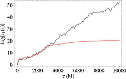
Figure 1: Rigorous Jacobian method compared to unrescaled deviation vector method for an $S=1$ particle in maximal ($a=1$) Kerr spacetime. The vertical axis is the natural logarithm of the largest principal axis $r_{1}$ of the phase space ellipsoid; the slope is the principal Lyapunov exponent, $\lambda_{\mathrm{max}}\approx 5\times 10^{-3}\,M^{-1}$. The unrescaled deviation vector method started with a deviation of size $10^{-7}$, and it saturates at $\sim\!\!16$. This corresponds to a growth of $e^{16}\approx 9\times 10^{6}$, which means that the separation has grown to a size of order unity. In conventional units, this indicates radial separations of order $GM/c^{2}$ and velocity separations of order $c$. The norm is calculated using the projected norm described in Sec. IV.2.

IV.2 The Papapetrou case

The discussion in the previous section was of a general nature, applicable to virtually any dynamical system described by differential equations. Here we describe some of the details needed to apply the general methods to the Papapetrou equations. In particular, we must discuss further the key ideas of constrained deviation vectors and phase space metric.

For the Papapetrou system, the phase space vector $\mathbf{y}$ has 12 components:

$${\mathbf{y}}=(t,r,\mu,\phi,p_{t},p_{r},p_{\theta},p_{\phi},S_{t},S_{r},S_{\mu},S_{\phi}).$$ (55)

The tangent vector $\bm{\xi}$ has one component for each variable. The set of equations Eq. (43) is simply the Papapetrou equations written out in full:

$$\dot{x}^{\mu} = v^{\mu}$$

$$\dot{p}_{\mu} = -R^{*\ \ \alpha\beta}_{\mu\nu}v^{\nu}p_{\alpha}S_{\beta}+\Gamma^{\alpha}_{\ \beta\mu}p_{\alpha}v^{\beta}$$

$$\dot{S}_{\mu} = -p_{\mu}\left(R^{*\alpha\ \gamma\delta}_{\ \ \beta}S_{\alpha}v^{\beta}p_{\gamma}S_{\delta}\right)+\Gamma^{\alpha}_{\ \beta\mu}S_{\alpha}v^{\beta},$$

where we have used the formulation in terms of the spin 1-form described in the appendix. The second necessary equation, Eq. (49), requires the Jacobian matrix,

$$\left(\begin{array}[]{rcl}\displaystyle{\frac{\partial\dot{x}^{\mu}}{\partial x^{\nu}}}&\displaystyle{\frac{\partial\dot{x}^{\mu}}{\partial p_{\nu}}}&\displaystyle{\frac{\partial\dot{x}^{\mu}}{\partial S_{\nu}}}\vskip 6.0pt plus 2.0pt minus 2.0pt\\ \displaystyle{\frac{\partial\dot{p}_{\mu}}{\partial x^{\nu}}}&\displaystyle{\frac{\partial\dot{p}_{\mu}}{\partial p_{\nu}}}&\displaystyle{\frac{\partial\dot{p}_{\mu}}{\partial S_{\nu}}}\vskip 6.0pt plus 2.0pt minus 2.0pt\\ \displaystyle{\frac{\partial\dot{S}_{\mu}}{\partial x^{\nu}}}&\displaystyle{\frac{\partial\dot{S}_{\mu}}{\partial p_{\nu}}}&\displaystyle{\frac{\partial\dot{S}_{\mu}}{\partial S_{\nu}}}\\ \end{array}\right),$$ (56)

whose explicit form appears in Hartl (2003).

It is important to mention that the tangent vector $\bm{\xi}$—or, equivalently, the deviation vector $\delta\mathbf{y}$—cannot have completely arbitrary components. On the contrary, the deviation must be chosen carefully, in order to ensure that, given a point $\mathbf{y}$ that satisfies the constraints from Sec. II.2, the deviated vector $\mathbf{y}+\delta\mathbf{y}$ also satisfies the constraints. Otherwise, the relation ${\bf f}({\bf y}+\delta{\bf y})-{\bf f}({\bf y})={\bf Df}\cdot\delta{\bf y}+{\cal O}(\|\delta{\bf y}\|^{2})$ is not satisfied. (This is the principal complication in implementing a rescaled version of the deviation vector method: the rescaled vector would violate the constraint.) In practice, we are able to find a valid deviation vector by applying the same techniques used to satisfy the constraints in the first place (Sec. III); for details, see Hartl (2003).

One final detail is the notion of metric: implicit in the definition of the Lyapunov exponent, Eq. (53), is a metric on phase space used to calculate the norm of the tangent vector $\bm{\xi}$. We adopt a metric introduced in Karas and Vokrouhlický (1992), which involves projecting the deviation vector onto the spacelike hypersurface defined by the zero angular momentum observers (ZAMOs). The projection is effected using the projection tensor $P^{\mu}_{\ \nu}=\delta^{\mu}_{\ \nu}+U^{\mu}U_{\nu}$, where $U^{\mu}$ is the ZAMO 4-velocity. The spatial and momentum variables are then projected according to $x^{\mu}\rightarrow\tilde{x}^{i}=P^{i}_{\ \mu}\,x^{\mu}$, $p_{\mu}\rightarrow\tilde{p}_{i}=P^{\mu}_{\ i}\,p_{\mu}$, and $S_{\mu}\rightarrow\tilde{S}_{i}=P^{\mu}_{\ i}\,S_{\mu}$. After the projection, we calculate the Euclidean norm in the 3-dimensional hypersurface. We note that while this prescription is convenient, and reduces correctly in the nonrelativistic limit, the magnitudes of the Lyapunov exponents are similar for several other possible choices of metric Hartl (2003).

IV.3 Chaos detector

Since we are concerned with calculating Lyapunov exponents for a large number of parameter values, we use the (unrescaled) deviation vector method because of its speed. As mentioned in Sec. IV.1, this method has the property of saturation (as illustrated in Fig. 1), which is ordinarily a problem, but here we use it to our advantage as a sensitive detector of chaos.

Our method for determining whether a particular initial condition is chaotic is to consider a nearby initial condition separated by a small vector $\delta\mathbf{y}_{0}$ (with norm $\|\delta\mathbf{y}_{0}\|$ typically of order $10^{-7}$ or $10^{-8}$) and then integrate until the system reaches 90% of the saturation limit, defined as a separation $\delta\mathbf{y}$ with unit norm. If we write $r_{e}=\|\delta\mathbf{y}\|/\|\delta\mathbf{y}_{0}\|$, the approximate Lyapunov exponent satisfies

$$\log{[r_{e}(\tau)]}=\lambda\tau,$$ (57)

so that $\lambda$ is the slope of the line $\log{[r_{e}(\tau)]}$ vs. $\tau$. Saturation occurs when $r_{e}=1/\|\delta\mathbf{y}_{0}\|$, so that the integration ends when $\log{[r_{e}(\tau)]}=-\log{(0.9\,\|\delta\mathbf{y}_{0}\|)}$. We record the value of $\log{[r_{e}(\tau)]}$ at regular time intervals (typically every time $T=100\,M$ in our case), and upon reaching 90% saturation perform a least-squares fit on the simulation data to determine the exponent.

We note that the cutoff value of $0.9$ is somewhat arbitrary and is the result of numerical experimentation. When using the (unrescaled) deviation vector approach, most of the chaotic systems saturate—that is, plots of $\log{[r_{e}(\tau)]}$ vs. $\tau$ flatten out (Fig. 1)—when the separation is of order unity, corresponding to radial separations of order $M$, velocity separations of order $1$, and angular separations of order $1~{}\mathrm{radian}$. The 90% prescription ends the integration before the growth flattens out, so that the numerical estimate for the exponent is still reasonably accurate.

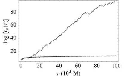
Figure 2: A comparison of chaotic and nonchaotic initial conditions. The slopes of the lines are the approximate Lyapunov exponents. Each initial condition shares the same values of $S=0.1$, $e=0.6$, and $r_{p}=1.21$. They differ only in inclination angle: $\iota=31^{\circ}$ (chaotic) and $\iota=28.5^{\circ}$ (not chaotic). Their respective Lyapunov exponents are $\lambda=1.0\times 10^{-3}\,M^{-1}$ and $\lambda=3.0\times 10^{-3}\,M^{-1}$. See Sec. V.2 for details.

For the large maps of parameter space, we typically integrate up to $\tau_{\mathrm{final}}=10^{5}\,M$ or saturation, whichever comes first. We choose this maximum time mainly for practical reasons: it is the longest integration possible in a reasonable amount of time. [We integrate as deeply as $10^{7}\,M$ (Sec. V.7) for individual orbits, but such long integrations are impractical for more than a handful of parameter combinations.] Dramatically longer integrations are also not particularly useful, since the timescale for gravitational radiation reaction is on the order of $\tau_{\mathrm{GW}}=M^{2}/\mu$ Hughes (2001), which for the most relevant LISA sources is $10^{4}$–$10^{6}\,M$ (i.e., $\mu\sim 10^{-6}$–$10^{-4}\,M$). Searching for chaos in such systems on a timescale longer than $\sim\!\!10^{7}\,M$ is probably pointless, since the radiation reaction would dominate the dynamics in this case. Finally, it appears that chaos, when present in the Papapetrou system, manifests itself on relatively short timescales ($10^{2}$–$10^{4}\,M$), or else not at all. The onset of chaos is marked by a qualitative change from power law growth (which appears as logarithmic growth on our plots of $\log{[r_{e}(\tau)]}$ vs. $\tau$) to exponential growth (which is linear on the same plots). An example of two similar initial conditions giving rise to qualitatively different dynamical behavior appears in Fig. 2.

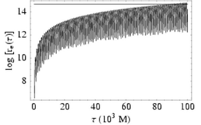
Figure 3: A chaos mimic: $\log{[r_{e}(\tau)]}$ vs. $\tau$ for an $S=0$ orbit. The size of the initial deviation vector is $\epsilon_{0}=3.3\times 10^{-7}$. The value of $\log{[r_{e}(\tau)]}$ periodically rises up to the saturation level (shown as a horizontal line at $14.82$, since $e^{14.82}\,\epsilon_{0}=0.9$). The system’s spin satisfies $S=0$, and is hence fully integrable, which implies no chaos. We detect such spurious chaos by demanding several saturation points in a row for a positive detection. The corresponding orbit appears in Fig. 22.

Figure 4: The difference $\delta r$ between the Boyer-Lindquist radii of two nearby trajectories for a chaos mimic. The growth in the separation is substantial, but not exponential. The initial conditions are the same as in Fig. 3.

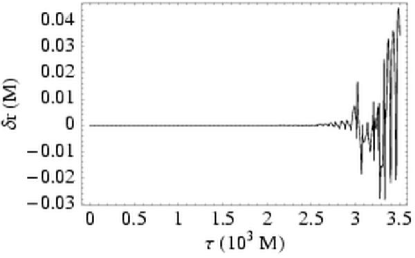
Figure 5: The difference $\delta r$ between the Boyer-Lindquist radii of two nearby trajectories for a chaotic orbit. The initial condition is taken from the inner region of Fig. 9 ($r_{p,\,K}=2.0$, $e_{K}=0.5$, $\iota_{K}=10^{\circ}$, $S=1$). On this linear scale, the separation seems to burst unexpectedly, in contrast to the relatively smooth linear growth for the nonchaotic orbit shown in Fig 4.

One important refinement to the technique described above is to require several 90% saturation points in a row before declaring the orbit to be chaotic. This is necessary because some nonchaotic orbits have very high amplitudes on plots of $\log{[r_{e}(\tau)]}$ vs. $\tau$ (Fig. 3). This phenomenon occurs mainly for orbits with many periods in the deeply relativistic zone near the horizon. Such orbits may reach “90% saturation” briefly as part of their oscillation, but quickly return to separations far below our chaotic cutoff. We therefore adopt the criterion of three 90% saturation points in a row (with a time $T=100\,M$ sampling interval) as a robust practical test for chaos. See Sec. V.8 for further discussion.

Our confidence of this method’s robustness derives from comparing the method above to the Jacobian method for the same initial conditions. Since the Jacobian method does not saturate, the agreement of the two methods indicates that our procedure provides an accurate detector for chaos (as in Fig. 12 below).

IV.4 Implementation notes

We integrate the Papapetrou equations on a computer using Bulirsch-Stoer and Runge-Kutta integrators implemented in the C programming language, as described in Hartl (2003). The derivatives and Jacobian matrix are extensively hand-optimized for speed. We monitor errors using constraints and conserved quantities, with a global error goal of $10^{-13}$. The errors are at the $10^{-11}$ level or better for highly chaotic orbits after $10^{5}\,M$. Orbits with low spin or high pericenter are even more accurate, often achieving the error goal of $10^{-13}$.

The many plots in Sec. V are typically generated using driver programs written in the Perl programming language, which in turns calls the C integrator repeatedly. This general paradigm—using an interpreted language such as Perl to call optimized routines in a compiled language such as C—is one we warmly recommend.

V Results

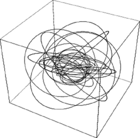
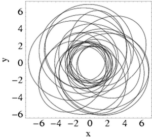
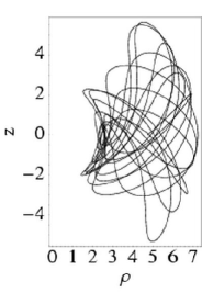
(a)		(b)		(c)

Figure 6: The orbit of a maximally spinning ($S=1$) test particle in maximal ($a=1$) Kerr spacetime, plotted in Boyer-Lindquist coordinates. (a) The orbit embedded in three-dimensional space, treating the Boyer-Lindquist coordinates as ordinary spherical polar coordinates; (b) $y=r\sin\theta\sin\phi$ vs. $x=r\sin\theta\cos\phi$; (c) $z$ vs. $\rho=\sqrt{x^{2}+y^{2}}$. The requested orbital inclination angle is $\iota=6^{\circ}$, but the strong spin coupling gives rise to an empirical value closer to $\iota_{P}=46^{\circ}$. The empirical pericenter is $r_{p}=2.219\,M$, which is fairly close to the requested value of $2.367\,M$.

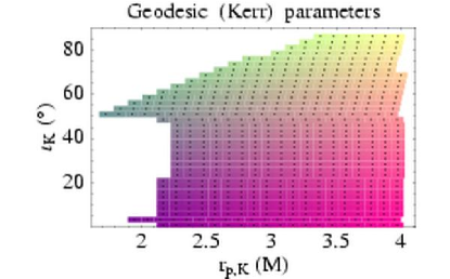
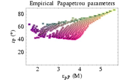
(a)	(b)

Figure 7: Shading/coloring of parameter space for an $S=1$ orbit. The shading/color on the left is repeated on the right, so that we can visually determine the mapping of $(r_{p,\,K},\iota_{K})$ to $(r_{p,\,P},\iota_{P})$. It is evident that orbits with low requested pericenters and orbital inclination angles are mapped to low-pericenter orbits at high inclinations, and the entire parameter space is compressed. Not that the gap in stable initial conditions visible in (b) is a true gap, not a fold.

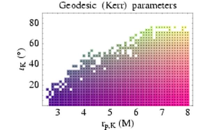
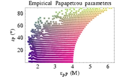
(a)	(b)

Figure 8: Shading/coloring of parameter space for an $S=1$ orbit illustrating the alternate parameterization method from Sec. III.2.2. As in Fig. 7, the shading/color on the left is repeated on the right. The spatial part of the initial spin is purely in the $z$ direction. The Kerr $p^{\theta}_{K}$ and Papapetrou $p^{\theta}_{P}$ values are forced to agree, which leads to similar inclination angles in parts (a) and (b), at the cost of dramatically different pericenters.

We present here the results of parameter variation in the Papapetrou system of equations. We represent the effects compactly using several different kinds of plots, most of which involve plotting inclination vs. pericenter, with other parameters held fixed. We refer to these as $r_{p}$-$\iota$ maps. As discussed in Sec. III, starting with the Kerr values $r_{p,\,K}$, $\iota_{K}$, and $e_{K}$, we find the corresponding energy $E_{K}$, angular momentum $L_{z,K}$, and Carter constant $Q_{K}$, and then force the Papapetrou values to satisfy $E_{P}=E_{K}$, $J_{z,P}=L_{z,K}$ and $p^{r}_{P}=p^{r}_{K}$. Each $r_{p}$-$\iota$ map has two components: part (a), shown on the left, uses the Kerr parameters $\iota_{K}$ and $r_{p,\,K}$ requested by the parameterization (Sec. III.2.2), while part (b), shown on the right, always shows the empirical Papapetrou values $\iota_{P}$ and $r_{p,\,P}$ in the sense of Sec. III.2.3.

One important feature of $r_{p}$-$\iota$ parameter space apparent in the empirical plots is the prevalence of large empirical inclination angles for all values of the Kerr inclination $\iota_{K}$. Fig. 7 shows the mapping for $S=1$ between the requested Kerr parameters [Fig. 7(a)] and the empirical Papapetrou parameters [Fig. 7(b)] using a shading scheme (which appears as a more informative color scale in electronic versions of this paper). We see that even the orbits at the bottom of Fig. 7(a) get mapped to high empirical inclination angles; $\iota_{K}=1^{\circ}$ orbits are mapped to inclinations of order $\iota_{P}=40^{\circ}$.

This compression of parameter space is the result of our choice to force the Kerr and Papapetrou value of the radial momentum to agree (Sec. III.2.2). The price we pay for this choice is that the $\theta$ component of the Papapetrou momentum—which is constrained to satisfy the equations in Sec. II.2—is relatively large. This high $p^{\theta}_{P}$ flings even orbits with low requested values of $\iota_{K}$ to high inclinations (Fig. 7). It is possible to find low-inclination Papapetrou orbits by requiring that the Kerr and Papapetrou values of $p^{\theta}$ agree, but at the cost of forcing $p^{r}$ to be very different—again a result of the constraints. The resulting parameter space (Fig. 8) is not nearly as compressed in inclination angle, but the Papapetrou pericenters are compressed and shifted down, and many requested values of $r_{p},\,K$ are lost as plunge orbits. In addition, the empirical values of the eccentricity are typically not close to the value requested (reaching, e.g., $e_{P}=0.75$ for $e_{K}=0.5$). Because of the deficiencies of this alternate parameterization method, we choose the fixed $p^{r}$ plots are our primary investigative tool in this paper.

V.1 Varying pericenter and orbital inclination

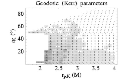
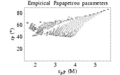
(a)	(b)

Figure 9: $r_{p}$-$\iota$ map for $a=1$, $e=0.5$, $S=1$, $S^{\hat{r}}=S^{\hat{z}}=0.2\,S$: chaos strength as a function of pericenter and orbital inclination angle. (a) Requested parameters; (b) empirical parameters. The initial conditions are the same as in Fig. 7. The rectangles are shaded according to the Lyapunov exponent for the initial condition represented by each point, with darker shades of gray representing larger exponents and hence stronger chaos. The point at $r_{p,\,K}=2.3$ and $\iota_{K}=20^{\circ}$ is one of the points in Fig. 17, which shows the effects of varying $S^{\hat{r}}$ and $S^{\hat{z}}$. The largest exponent in this plot is $\lambda=4.1\times 10^{-3}\,M^{-1}$, corresponding to a timescale of $1/\lambda=2.4\times 10^{2}\,M$ for a factor of $e$ divergence in nearby initial conditions.

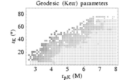
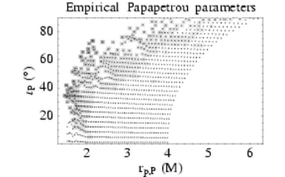
(a)	(b)

Figure 10: $r_{p}$-$\iota$ map for $a=1$, $e=0.5$, $S=1$, using the alternate parameterization method that forces $p_{K}^{\theta}=p_{P}^{\theta}$. The initial spatial component of the spin is purely in the $z$ direction. (a) Requested parameters; (b) empirical parameters. The initial conditions are the same as in Fig. 8. The rectangles are shaded according to the Lyapunov exponent for the initial condition represented by each point, with darker shades of gray representing larger exponents and hence stronger chaos. The largest exponent in this plot is $\lambda=4.0\times 10^{-3}\,M^{-1}$, corresponding to a timescale of $1/\lambda=2.5\times 10^{2}\,M$ for a factor of $e$ divergence in nearby initial conditions. These values are virtually identical to the values in Fig. 9.

In this section we show $r_{p}$-$\iota$ maps for orbits with fixed eccentricity $e=0.5$ and spin parameters $S^{\hat{r}}=S^{\hat{z}}=0.2\,S$, where $S$ is the total spin. We indicate the strength of the chaos at each point with a grayscale rectangle, with the darkest colors representing the strongest chaos (and with white indicating no chaos). An example of such a plot appears in Fig. 9. (Fig. 10 shows a similar plot for the alternate parameterization method that forces $p_{K}^{\theta}=p_{P}^{\theta}$. The maximum exponents in the two cases are virtually identical.) The most important general results evident from the plots are two-fold. First, the largest exponents occur for orbits with pericenters deep in the relativistic zone near the horizon. Second, the prevalence of chaotic orbits is a decreasing function of spin parameter $S$, with virtually all chaos gone by the time $S=0.1$.

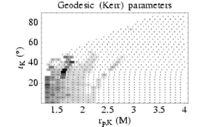
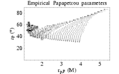
(a)	(b)

Figure 26: $r_{p}$-$\iota$ map for $S=0.5$, $a=1$, and $e=0.5$. (a) Requested parameters; (b) empirical parameters. The shading is scaled to the same maximum Lyapunov exponent as Fig. 9. Because of the extremely low pericenters accessible at this value of $S$ (which are excluded when $S=1$), the chaos for $S=0.5$ is the strongest we find. The largest Lyapunov exponent is just over $\lambda=0.01\,M^{-1}$.

An example of the value of the empirical $r_{p,\,P}$-$\iota_{P}$ plots appears in Fig. 26, which shows orbits of particles with spin $S=0.5$. The appearance of a strongly chaotic point in Fig. 26 seems perplexing, given that it is surrounded but many points with much smaller exponents. As is evident from the empirical plot, this point of strong chaos (which is, in fact, the largest Lyapunov exponent for any of the plots) maps to a compressed area of initial conditions with small empirical pericenters [Fig. 26(b)].

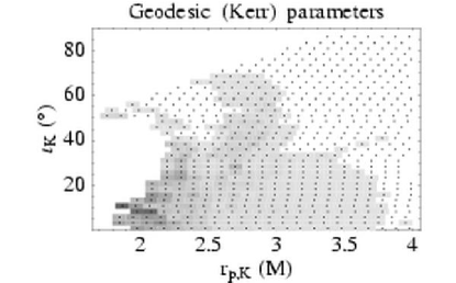
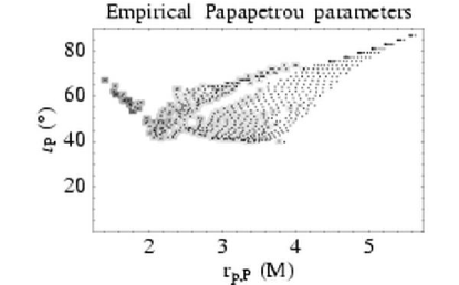
(a)	(b)

Figure 25: $r_{p}$-$\iota$ map for $S=0.9$, $a=1$, and $e=0.5$. (a) Requested parameters; (b) empirical parameters. The shading is scaled to the same maximum Lyapunov exponent as Fig. 9. Chaotic orbits are widespread.

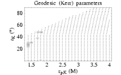
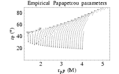
(a)	(b)

Figure 27: $r_{p}$-$\iota$ map for $S=0.2$, $a=1$, and $e=0.5$. (a) Requested parameters; (b) empirical parameters. The shading is scaled to the same maximum Lyapunov exponent as Fig. 9. Only a few orbits are chaotic.

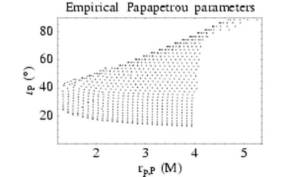
(a)	(b)

Figure 28: $r_{p}$-$\iota$ map for $S=0.1$, $a=1$, and $e=0.5$. (a) Requested parameters; (b) empirical parameters. The shading is scaled to the same maximum Lyapunov exponent as Fig. 9. All chaos is gone, although the parameter space is still somewhat compressed.

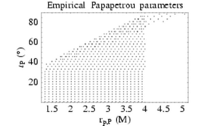
(a)	(b)

Figure 29: $r_{p}$-$\iota$ map for $S=10^{-4}$, $a=1$, and $e=0.5$. (a) Requested parameters; (b) empirical parameters. The shading is scaled to the same maximum Lyapunov exponent as Fig. 9. There are no chaotic orbits. The empirical parameter values in (b) are indistinguishable from the requested values except for initial conditions that specify values of $\iota$ corresponding to unstable orbits (as discussed in Sec. III.2.3).

From an astrophysical standpoint, the most interesting parameter to vary is the spin $S$, since only $S\ll 1$ orbits are physically realistic (Sec. II.4). From Figs. 25–29, which involve varying $S$ from 0.9 down to $10^{-4}$, we see that both the prevalence and strength of chaos decrease significantly as $S$ is decreased. The Lyapunov exponent ranges as high as $10^{-2}\,M^{-1}$ when $S=0.5$ (Fig. 26), but the chaos is weak when $S=0.2$ (Fig. 27) and is gone below $S=0.1$ (Figs. 28 and 29).

V.2 Varying eccentricity

The choice of $e=0.5$ in the previous section is partially motivated by likely gravitational wave sources for LISA LIS , e.g., a neutron star or small black hole in an eccentric orbit around a supermassive black hole. In this section, we consider a second series of eccentric orbits at fixed $e=0.6$ and varying spin parameter. We also investigate the case of a near-circular orbit ($e=0.01$) more appropriate for the circularized gravitational wave sources important for ground-based detectors such as LIGO.

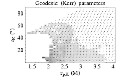
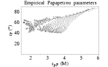
(a)	(b)

Figure 30: $r_{p}$-$\iota$ map for $S=1$, $a=1$, and $e=0.6$. (a) Requested parameters; (b) empirical parameters. The shading is scaled to the same maximum Lyapunov exponent as Fig. 9. Chaotic orbits are widespread. The largest Lyapunov exponent is $\lambda=5.5\times 10^{-3}\,M^{-1}$.

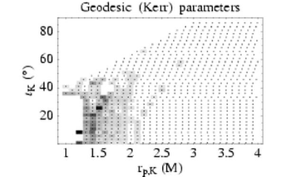
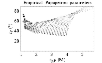
(a)	(b)

Figure 31: $r_{p}$-$\iota$ map for $S=0.5$, $a=1$, and $e=0.6$. (a) Requested parameters; (b) empirical parameters. The shading is scaled to the same maximum Lyapunov exponent as Fig. 9. As in the case of Fig. 26, the low accessible pericenters give rise to strong chaos. The largest Lyapunov exponent is $\lambda=9.2\times 10^{-3}\,M^{-1}$.

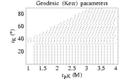
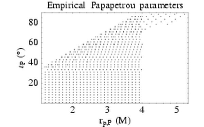
(a)	(b)

Figure 33: $r_{p}$-$\iota$ map for $S=10^{-4}$, $a=1$, and $e=0.6$. (a) Requested parameters; (b) empirical parameters. The shading is scaled to the same maximum Lyapunov exponent as Fig. 9. All chaos has disappeared. As in Fig. 29, the empirical parameter values in (b) are indistinguishable from the requested values except for initial conditions that specify unstable orbits (Sec. III.2.3).

The $r_{p}$-$\iota$ plots for $e=0.6$ follow the same pattern as those with $e=0.5$. Chaos is strongest for orbits with small pericenters and values of $S$ of order unity (Figs. 30–33). There is a single orbit at $S=0.1$ that appears to be chaotic (Fig. 32), but other than this one exception there is apparently no chaos below $S=0.1$. A close examination of the single $S=0.1$ chaotic orbit appears in Figs. 11–12, which shows that the chaos is real.

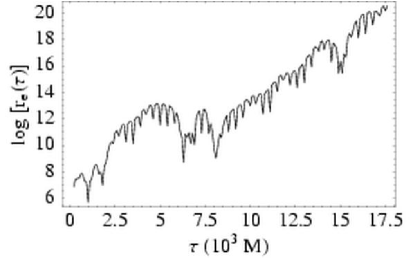
Figure 11: Natural logarithm of the largest ellipsoid axis vs. time. We use the unrescaled deviation vector method to investigate the single chaotic initial condition from Fig. 32, which has $r_{p,\,K}=1.21$, $e_{k}=0.6$, $\iota_{K}=31^{\circ}$, and $S=0.1$. The principal ellipsoid axis grows until it saturates at $\tau=17600\,M$.

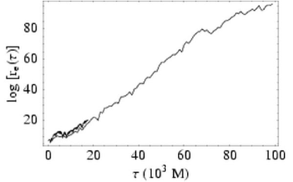
Figure 12: Natural logarithm of the largest ellipsoid axis vs. time using the unrescaled deviation vector method and the rigorous Jacobian method. The unrescaled integration is identical to that shown in Fig. 11. The two methods agree until the deviation method saturates, at which point we stop the deviated vector integration. The continued growth of the Jacobian method confirms that the orbit determined by the initial condition is indeed chaotic.

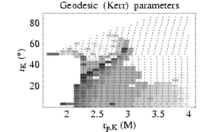
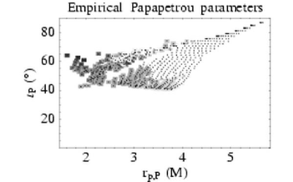
(a)	(b)

Figure 13: Spin cutoff map for $a=1$ and $e=0.5$. The rectangles are shaded according to the minimum value of $S$ for which the corresponding initial condition is still chaotic. White rectangles indicate points that are not chaotic even when $S=1$. The darkest points correspond to a cutoff value of $S=0.18457$; below this critical value, none of the initial conditions are chaotic.

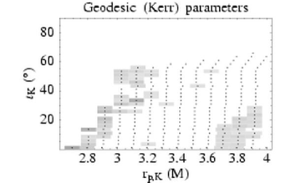
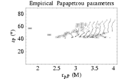
(a)	(b)

Figure 34: $r_{p}$-$\iota$ map for $S=1$, $a=1$, and $e=0.01$. (a) Requested parameters; (b) empirical parameters. The shading is scaled to the same maximum Lyapunov exponent as Fig. 9. There is some relatively weak chaos. The largest Lyapunov exponent is $\lambda=2.7\times 10^{-3}\,M^{-1}$.

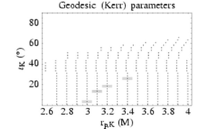
(a)	(b)

Figure 35: $r_{p}$-$\iota$ map for $S=0.5$, $a=1$, and $e=0.01$. (a) Requested parameters; (b) empirical parameters. The shading is scaled to the same maximum Lyapunov exponent as Fig. 9. There are a few regions of weak chaos.

The effect of chaos is smaller for the near-circular ($e=0.01$) orbits considered (Figs. 34–37), with typical Lyapunov exponents of order $2\times 10^{-3}\,M^{-1}$ when $S=1$ (Fig 34). Moreover, we find only four points with nonzero exponents for $S=0.5$ (Fig. 35), in contrast to the more eccentric orbits, which have strong chaos for $S=0.5$. By the time $S=0.1$ (Fig. 36), all chaos has completely disappeared for the near-circular orbits.

V.3 Varying Kerr parameter $a$

Here we investigate the effect of the Kerr parameter $a$ on the strength and prevalence of chaos. Although Suzuki & Maeda found in Suzuki and Maeda (1997) that there is chaos even in Schwarzschild spacetime, to which Kerr spacetime reduces when $a=0$, the chaotic orbits found in Suzuki and Maeda (1997) are exceptional orbits lying on the edge of a generalized effective potential. We found evidence in Hartl (2003) that such chaotic orbits are rare.

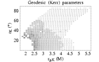
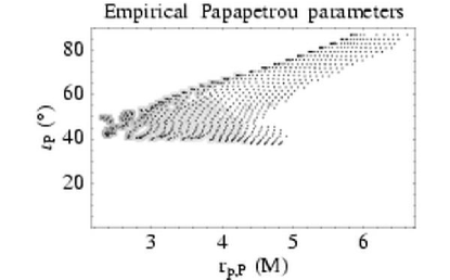
(a)	(b)

Figure 38: $r_{p}$-$\iota$ map for $S=1$, $a=0.9$, and $e=0.5$. (a) Requested parameters; (b) empirical parameters. The shading is scaled to the same maximum Lyapunov exponent as Fig. 9. Chaotic orbits are widespread.

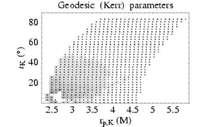
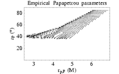
(a)	(b)

Figure 39: $r_{p}$-$\iota$ map for $S=1$, $a=0.7$, and $e=0.5$. (a) Requested parameters; (b) empirical parameters. The shading is scaled to the same maximum Lyapunov exponent as Fig. 9. There is still substantial chaos.

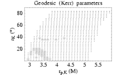
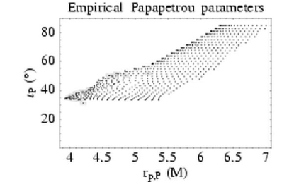
(a)	(b)

Figure 40: $r_{p}$-$\iota$ map for $S=1$, $a=0.5$, and $e=0.5$. (a) Requested parameters; (b) empirical parameters. The shading is scaled to the same maximum Lyapunov exponent as Fig. 9. The chaos is largely confined to low pericenter orbits.

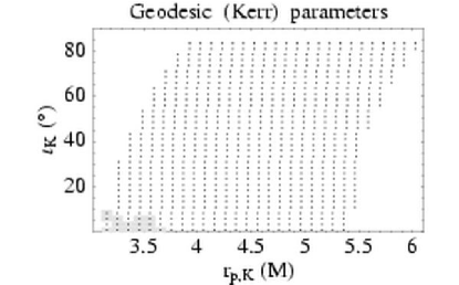
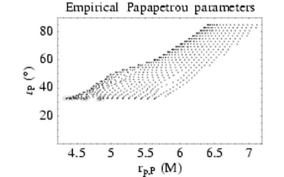
(a)	(b)

Figure 41: $r_{p}$-$\iota$ map for $S=1$, $a=0.4$, and $e=0.5$. (a) Requested parameters; (b) empirical parameters. The shading is scaled to the same maximum Lyapunov exponent as Fig. 9. Only a handful of initial conditions are chaotic.

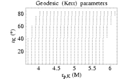
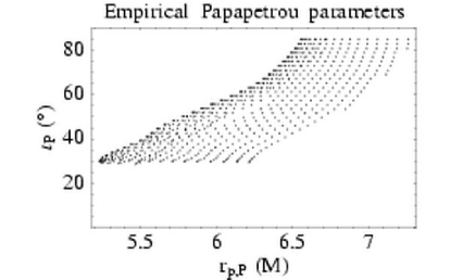
(a)	(b)

Figure 42: $r_{p}$-$\iota$ map for $S=1$, $a=0.2$, and $e=0.5$. (a) Requested parameters; (b) empirical parameters. The shading is scaled to the same maximum Lyapunov exponent as Fig. 9. No initial conditions are chaotic.

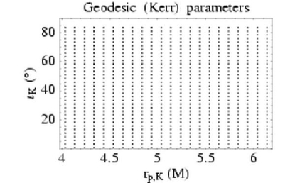
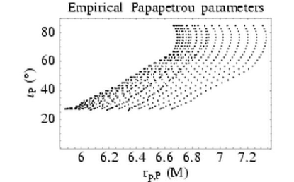
(a)	(b)

Figure 43: $r_{p}$-$\iota$ map for $S=1$, $a=0$, and $e=0.5$. (a) Requested parameters; (b) empirical parameters. The shading is scaled to the same maximum Lyapunov exponent as Fig. 9. No initial conditions are chaotic. Note that every column of (a) is identical. This is a result of the spherical symmetry of the $a=0$ (Schwarzschild) metric: all inclination angles are equivalent. As seen in (b), this symmetry is broken by the spin of the test particle.

The conclusion that chaotic orbits become less prevalent as $a\rightarrow 0$ is supported by a more thorough examination, as illustrated in Figs. 38–43. All of these orbits have eccentricity $e=0.5$ and spin $S=1$, and $a$ varies from $0.9$ down to 0. Even for low values of $a$, the parameter space is strongly affected by the spin, with plots of the empirical pericenter and orbital inclination showing significant distortion. Nevertheless, we see unambiguously that the chaotic orbits prevalent when $a=1$ are greatly suppressed as $a$ decreases, with no chaotic orbits at all below $a=0.2$. This appears to be a result of the increase of the marginally stable radius $r_{\mathrm{ms}}$ as $a\rightarrow 0$. When $a=0$, the minimum stable radius is at $r_{\mathrm{ms}}=4$ in units of the central black hole’s mass, fully $2\,M$ away from the horizon at $r_{H}=2\,M$. As discussed in Hartl (2003), the extra (spherical) symmetry of the Schwarzschild metric leads to an additional integral of the motion, which also has a suppressive effect on chaos.

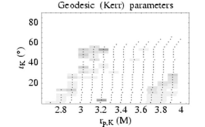
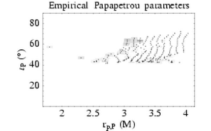
(a)	(b)

Figure 14: Spin cutoff map for $a=1$ and $e=0.01$. The rectangles are shaded according to the minimum value of $S$ for which the corresponding initial condition is still chaotic. White rectangles indicate points that are not chaotic even when $S=1$. The darkest points correspond to a cutoff value of $S=0.65625$; below this critical value, none of the initial conditions are chaotic.

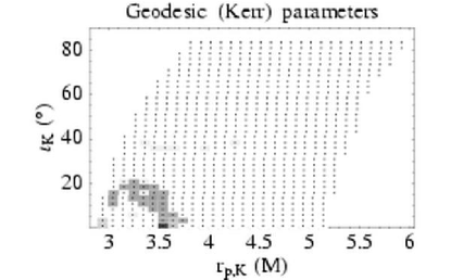
(a)	(b)

Figure 15: Spin cutoff map for $a=0.5$ and $e=0.5$. The rectangles are shaded according to the minimum value of $S$ for which the corresponding initial condition is still chaotic. White rectangles indicate points that are not chaotic even when $S=1$. The darkest points correspond to a cutoff value of $S=0.28125$; below this critical value, none of the initial conditions are chaotic.

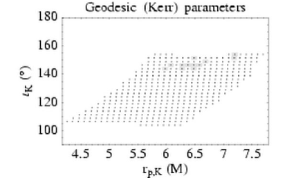
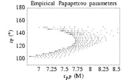
(a)	(b)

Figure 16: $r_{p}$-$\iota$ map of retrograde orbits ($\iota>90^{\circ}$) for $a=1$, $e=0.5$, $S=1$: chaos strength as a function of pericenter and orbital inclination angle. (a) Requested parameters; (b) empirical parameters. The rectangles are shaded according to the Lyapunov exponent for the initial condition represented by each point, with darker shades of gray representing larger exponents and hence stronger chaos. The scaling is the same as Fig. 9; an exponent of $\lambda=0.01\,M^{-1}$ would appear black. The chaos is weak for these retrograde orbits: the largest Lyapunov exponent in the plot is $\lambda=3.5\times 10^{-4}\,M^{-1}$.

V.4 Spin cutoffs for chaos

In this section we provide spin cutoff values for chaos, i.e., the minimum spin values for which chaos exists. For a given initial condition defined in terms of fixed orbital parameters (as described in Sec. III.2), we vary the spin parameter $S$ and find the maximum value for which chaos occurs. The smaller this cutoff value, the stronger the chaos: nonchaotic orbits have a cutoff value of $S=1$, i.e., they are not chaotic even in the extreme $S=1$ limit; conversely, a cutoff value of $S=10^{-5}$ would indicate chaos for the (physically realistic) value $S=10^{-5}$, but not for any smaller values.

Fig. 13 is an example of a spin cutoff map. The procedure for producing such a map is similar to the method used to make the Lyapunov $r_{p}$-$\iota$ maps: we consider a grid of points in $r_{p}$-$\iota$ space, and for each point we find an approximate value for the spin cutoff. We begin by finding out if the system is chaotic for $S=1$, using the Lyapunov map as a start. If the orbit for $S=1$ is chaotic, we halve the spin value and calculate the Lyapunov exponent for $S=0.5$. If the system is still chaotic, we consider $S=0.25$; otherwise, we consider $S=0.75$. The procedure continues until the difference between chaotic and nonchaotic spin values is smaller than some threshold, which we choose to be $0.05$. (This value is chosen to achieve reasonable accuracy while still completing the calculations in a tolerable amount of time.)

Figs. 13–15 show the spin cutoff values for several parameter combinations corresponding to Lyapunov maps from Sec. V.1 above. The plots are color-coded with grayscale so that the most chaotic points—those with the smallest spin cutoff values—appear darkest. The points surrounded by white are not chaotic even for $S=1$. The cutoffs for the darkest points depend on the parameter values: for Fig. 13 ($a=1$ and $e=0.5$), the same as Fig. 9 above), we find $S_{\mathrm{cutoff}}=0.18457$; Fig. 14 ($a=1$ and $e=0.01$, the same as Fig. 34 above) has $S_{\mathrm{cutoff}}=0.65625$; and Fig. 15 ($a=0.5$ and $e=0.5$, the same as Fig. 40) has $S_{\mathrm{cutoff}}=0.28125$. We should not take the digits of precision seriously, since these values are only accurate to within $0.05$, but in all cases the spin cutoff values are significantly above the physically realistic range of $S\sim 10^{-4}$–$10^{-7}$.

V.5 Retrograde orbits

We have considered a wide variety of orbits—varying eccentricity and Kerr parameter for different pericenter, orbital inclination, and spin parameters—but so far all orbits have satisfied $0<\iota<\pi/2$, i.e., they have all been prograde orbits, moving in the same direction as the central black hole’s spin. We investigate now the case of retrograde orbits, and show that they are poor candidates for chaos.

It is evident from looking at an $r_{p}$-$\iota$ plot of a retrograde orbit (Fig. 16) that the pericenters are much larger than their prograde counterparts. For the $S=1$ particle illustrated in Fig. 16, the minimum empirical pericenter is larger than $6\,M$, in contrast to prograde orbits, which get below $1.5\,M$. Furthermore, although it is clear from Fig. 16(b) that the parameter space is severely distorted, the chaos is extremely weak. The largest Lyapunov exponent, even in this extreme $S=1$ case, is $\lambda_{\mathrm{max}}=3.5\times 10^{-4}$, two orders of magnitude smaller than the prograde case. Unsurprisingly, all chaos disappears when $S\ll 1$. The smallest value of $S_{\mathrm{cutoff}}$ is $0.65265$ for the parameter values shown in Fig. 16; we find no evidence of chaos below this value of $S$.

V.6 Varying spin inclination

So far we have always used the same values for the two spin components passed to the parameterization procedure (scaled by the total spin $S$): $S^{\hat{r}}=S^{\hat{z}}=0.2\,S$. We consider now the effect of varying these parameters, and also discuss the corresponding initial spin inclination angles in a fiducial rest frame.

We begin with an initial condition that is chaotic for $S=1$ but is otherwise arbitrary. We then vary $S^{\hat{r}}$ and $S^{\hat{z}}$ and calculate the Lyapunov exponent for each configuration. The result for $a=1$, $e_{K}=0.5$, $r_{p,\,K}=2.3$ and $\iota_{K}=20^{\circ}$ appears in Fig. 17. When $S^{\hat{r}}=S^{\hat{z}}=0.2$, the parameter values chosen correspond to a point from Fig. 9. There are not valid initial conditions for all choices of parameter; in particular, negative values of $S^{\hat{z}}$ are often unstable or are unable to satisfy the spin constraints. Nevertheless, there is a large variety of parameters that do give rise to valid orbits, and many of them are chaotic. The strongest chaos exists for orbits that have small values of $S^{\hat{z}}$, but this appears to be mainly because such orbits are able to achieve small empirical pericenters. As Fig. 18 clearly shows, the Lyapunov exponent generally decreases as pericenter increases, with no chaotic orbits above $r_{p,\,P}=2.5\,M$.

While we are forced by the constraints to parameterize the equations of motion in terms of spin components, it is more convenient to visualize the spin in a fiducial rest frame that is hypersurface-orthogonal to the particle’s trajectory. In Kerr spacetime, the hypersurface-orthogonal observers are the zero angular momentum observers (ZAMO), which is the same frame we use when calculating the Lyapunov exponents. By projecting the components of the spin vector $S^{\mu}$ into the ZAMO frame in the same way as we do for the projected norm (Sec. IV.2), we can find the local value of the spin inclination angle $\theta_{\mathrm{local}}$ (i.e., the angle between the spin axis and the axis of the central black hole). The results appear in Table 1. It is clear that our variation of spin components samples a large variety of initial spin inclination angles.

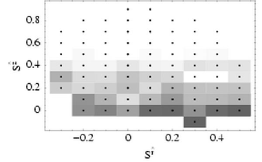
(a)

Figure 17: Lyapunov exponents for varying values of initial spin components $S^{\hat{r}}$ and $S^{\hat{z}}$. The parameter values $S=1$, $r_{p,\,K}=2.3$, $e_{K}=0.5$, and $\iota_{K}=20^{\circ}$ are held fixed. The point with $S^{\hat{r}}=S^{\hat{z}}=0.2$ appears in Fig. 9 above. The actual local spin inclination angles in a fiducial (ZAMO) rest frame appear in Table 1. Note that only one valid initial condition exists for negative initial $S^{\hat{z}}$.

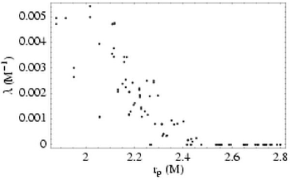
Figure 18: Scatter plot of empirical pericenters $r_{p,\,P}$ vs. Lyapunov exponent for the spin inclinations in Fig. 17. The Lyapunov exponent is primarily a function of pericenter, regardless of spin inclination.

Table 1: Local spin inclination angles $\theta_{\mathrm{local}}$ in a fiducial (ZAMO) rest frame as a function of $S^{\hat{r}}$ and $S^{\hat{z}}$. The parameter values $S=1$, $r_{p,\,K}=2.3$, $e_{K}=0.5$, and $\iota_{K}=20^{\circ}$ are held fixed. An illustration of their Lyapunov exponents appears in Fig. 17.

$S^{\hat{r}}$
$S^{\hat{z}}$	-0.3	-0.2	-0.1	0	0.1	0.2	0.3	0.4	0.5
0.9				$22.7^{\circ}$	$28.7^{\circ}$
0.8		$48.6^{\circ}$	$40.4^{\circ}$	$36.1^{\circ}$	$40.2^{\circ}$	$48.4^{\circ}$	$55.9^{\circ}$
0.7	$60.7^{\circ}$	$54.4^{\circ}$	$47.8^{\circ}$	$44.7^{\circ}$	$47.9^{\circ}$	$54.5^{\circ}$	$60.8^{\circ}$	$65.7^{\circ}$
0.6	$64.9^{\circ}$	$59.6^{\circ}$	$54.2^{\circ}$	$51.7^{\circ}$	$54.5^{\circ}$	$59.9^{\circ}$	$65.2^{\circ}$	$69.3^{\circ}$
0.5	$69.1^{\circ}$	$64.6^{\circ}$	$60.2^{\circ}$	$58.2^{\circ}$	$60.5^{\circ}$	$65.0^{\circ}$	$69.4^{\circ}$	$72.8^{\circ}$
0.4	$73.2^{\circ}$	$69.6^{\circ}$	$66.0^{\circ}$	$64.4^{\circ}$	$66.3^{\circ}$	$70.0^{\circ}$	$73.5^{\circ}$	$76.3^{\circ}$	$78.4^{\circ}$
0.3	$77.3^{\circ}$	$74.6^{\circ}$	$71.8^{\circ}$	$70.5^{\circ}$	$72.0^{\circ}$	$74.9^{\circ}$	$77.6^{\circ}$	$79.7^{\circ}$	$81.3^{\circ}$
0.2	$81.5^{\circ}$	$79.6^{\circ}$	$77.7^{\circ}$	$76.8^{\circ}$	$77.9^{\circ}$	$79.8^{\circ}$	$81.7^{\circ}$	$83.1^{\circ}$	$84.2^{\circ}$
0.1		$84.7^{\circ}$	$83.7^{\circ}$	$83.3^{\circ}$	$83.9^{\circ}$	$84.9^{\circ}$	$85.8^{\circ}$	$86.5^{\circ}$	$87.1^{\circ}$
0.0		$90.0^{\circ}$	$90.0^{\circ}$	$90.0^{\circ}$	$90.0^{\circ}$	$90.0^{\circ}$	$90.0^{\circ}$	$90.0^{\circ}$	$90.0^{\circ}$
-0.1							$94.2^{\circ}$

V.7 Deep integrations

Since we adopted a maximum time of $10^{5}\,M$ for the Lyapunov integrations, it is reasonable to ask whether chaos might manifest itself on a longer timescale. This is certainly possible, but it appears that most initial conditions are either chaotic on a timescale of order $10^{2}$–$10^{4}\,M$ or are not chaotic at all, as discussed in Sec. IV.3. An example appears in Fig. 2, where one initial condition is unambiguously chaotic, while a second located close by is not chaotic, even on a much longer timescale.

To convince ourselves that slow chaos is not lurking in the apparently nonchaotic regions, we performed a few longer-time integrations. In particular, we calculated the Lyapunov exponents using $\tau_{\mathrm{final}}=10^{7}\,M$ for all the innermost ($r_{p}=1.32$) orbits from Fig. 28 ($S=0.1$) and Fig. 29 ($S=10^{-4}$), which are strongly chaotic when $S=1$ but are apparently without chaos below $S=0.1$. The largest exponent occurs for $\iota=28.5^{\circ}$, which is therefore the worst-case scenario. Plots of the Lyapunov exponents vs. time appear in Fig. 19 ($S=0.1$) and Fig. 20 ($S=10^{-4}$); their magnitudes are on the order of $\lambda_{\mathrm{max}}=3\times 10^{-7}\,M^{-1}$, corresponding to an $e$-folding timescale of approximately $3.3\times 10^{6}\,M$. For comparison, we show $\lambda$ vs. $\tau$ for a chaotic initial condition in Fig. 21; it is clear that the Lyapunov exponent asymptotes to a nonzero value in much less than $10^{5}\,M$, even for weak chaos. (The initial condition in Fig. 21 is the $S=0.1$ orbit illustrated in Figs. 11 and 12, whose Lyapunov exponent is actually quite small compared to analogous $S=1$ orbits.) The long integrations thus provide strong evidence that the disappearance of nearly all chaotic orbits below $S=0.1$ is a real effect.

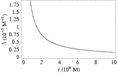
Figure 19: Approximate Lyapunov exponent vs. time for a nonchaotic deep ($\tau_{\mathrm{final}}=10^{7}\,M$) integration. The parameter values are $a=1$, $S=0.1$, $e=0.5$, $r_{p}=1.32\,M$, and $\iota=28.5^{\circ}$, corresponding to one of the inner orbits from Fig. 28. The Lyapunov exponent appears to be zero; its time-evolution has the characteristic hyperbolic shape expected as $\log{[r_{e}(\tau)]}/\tau$ approaches zero for large times. A least-squares fit of $\log{[r_{e}(\tau)]}$ vs. $\tau$ gives a value of $\lambda\approx 2.8\times 10^{-7}\,M^{-1}$.

Figure 20: Approximate Lyapunov exponent vs. time for a nonchaotic deep ($\tau_{\mathrm{final}}=10^{7}\,M$) integration. The parameter values are $a=1$, $S=10^{-4}$, $e=0.5$, $r_{p}=1.32\,M$, and $\iota=28.5^{\circ}$, corresponding to one of the inner orbits from Fig. 29. As in Fig. 19, the Lyapunov exponent appears to be zero. A least-squares fit of $\log{[r_{e}(\tau)]}$ vs. $\tau$ gives a value of $\lambda\approx 3.0\times 10^{-7}\,M^{-1}$.

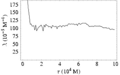
Figure 21: Approximate Lyapunov exponent vs. time for a chaotic deep ($\tau_{\mathrm{final}}=10^{5}\,M$) integration. The simulation data is identical to that shown in Fig. 12; the parameter values are $a=1$, $S=0.1$, $e_{K}=0.6$, $r_{p,\,K}=1.21\,M$, and $\iota_{K}=31^{\circ}$, corresponding to the chaotic orbit from Fig. 32. The Lyapunov exponent for this chaotic orbit levels off after less than $10^{5}\,M$, in contrast to Figs. 19 and 20, where $\lambda$ continues to decrease even after $10^{7}\,M$.

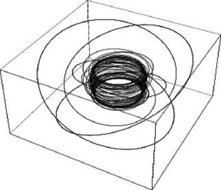
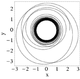
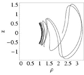
(a)		(b)		(c)

Figure 22: The orbit of a chaos mimic: a non-spinning ($S=0$) test particle in maximal ($a=1$) Kerr spacetime, plotted in Boyer-Lindquist coordinates. A Lyapunov plot of these initial conditions appears in Fig. 3 from Sec. IV.3. (a) The orbit embedded in three-dimensional space, treating the Boyer-Lindquist coordinates as ordinary spherical polar coordinates; (b) $y=r\sin\theta\sin\phi$ vs. $x=r\sin\theta\cos\phi$; (c) $z$ vs. $\rho=\sqrt{x^{2}+y^{2}}$. The inclination angle is $\iota=31^{\circ}$, while the pericenter is $r_{p}=1.1\,M$ (just $0.1\,M$ above the horizon at $r_{H}=1\,M$).

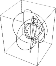
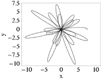
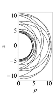
(a)		(b)		(c)

Figure 23: Another chaos mimic: a non-spinning ($S=0$) test particle in maximal ($a=1$) Kerr spacetime, plotted in Boyer-Lindquist coordinates. A Lyapunov plot of these initial conditions appears in Fig. 24. (a) The orbit embedded in three-dimensional space, treating the Boyer-Lindquist coordinates as ordinary spherical polar coordinates; (b) $y=r\sin\theta\sin\phi$ vs. $x=r\sin\theta\cos\phi$; (c) $z$ vs. $\rho=\sqrt{x^{2}+y^{2}}$. The inclination angle is $\iota=88.5^{\circ}$, while the pericenter is $r_{p}=4.4\,M$.

V.8 $S=0$ and chaos mimics

Since the case of $S=0$ corresponds exactly to geodesic orbits in Kerr spacetime, such systems cannot be chaotic—the return of the Carter constant $Q$ and the loss of the spin degrees of freedom make the system fully integrable. Nevertheless, even some geodesic orbits can have a large separation of nearby initial conditions, which can appear to be chaotic. These chaos mimics typically spend many orbital periods whirling around deep in the strongly relativistic zone near the horizon, only occasionally zooming out to higher radii. These so-called zoom-whirl orbits may provide significant challenges to detection despite their formal integrability.

An example of how much divergence an $S=0$ orbit can experience appears in Fig. 3. A picture of the corresponding orbit (visualized in Boyer-Lindquist coordinates embedded in ordinary space) appears in Fig. 22, which makes clear the large number of low-radius $\phi$-periods characteristic of zoom-whirl orbits. A second example of a chaos mimic appears in Figs. 24 and 23. This orbit, in contrast to the previous one, does not have a particularly small pericenter, but its high inclination angle and zoom-whirliness allow it to mimic chaotic orbits.

The chaos mimics can exhibit large growth of the initial deviation vector, approximately a factor of $10^{6}$–$10^{8}$, after $10^{5}\,M$. The principal means for detecting them is by requiring several high-separation points in a row (on a time-$T\approx 100\,M$ basis) as mentioned in Sec. IV.3; the mimics have oscillations with high amplitudes due to their zoom-whirliness, but they do not represent true saturations of the separation vector.

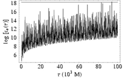
Figure 24: A chaos mimic: the natural logarithm of the principal ellipsoid axis ($\log{[r_{e}(\tau)]}$) vs. $\tau$ for an $S=0$ orbit. The size of the initial deviation vector is $\epsilon_{0}=10^{-8}$. The value of $\log{[r_{e}(\tau)]}$ briefly rises up to the saturation level at $\log(0.9/\epsilon_{0})$ [so that $\epsilon(\tau)=0.9$], but the orbit is not chaotic since its spin satisfies $S=0$. A plot of the corresponding orbit appears in Fig. 23.

VI Conclusions

The Papapetrou equations, which model a spinning test particle, exhibit chaotic solutions in Kerr spacetime for a wide range of parameters. In terms of the mass $M$ of the central (Kerr) black hole, the largest Lyapunov exponents are of order $\lambda_{\mathrm{max}}=0.01\,M^{-1}$, which represents an exponential divergence of trajectories on a timescale of $\tau_{\lambda}=1/\lambda=100\,M$. Furthermore, there are many chaotic orbits with exponents in the range $10^{-3}$–$10^{-4}\,M^{-1}$. Despite the large number of chaotic orbits, we find that values of $\lambda$ corresponding to unambiguous chaos occur exclusively when the spin parameter $S$ is not small compared to unity. In particular, we find virtually no chaos for spin values below $S=0.1$, and no evidence of any chaos for spins below $S=10^{-4}$.

The strongest determinant of chaotic behavior, apart from the spin parameter, is the pericenter of the orbit in question. The most highly chaotic orbits are those that reach pericenters near the horizon of the black hole. This is due to the high spacetime curvature in these regions, which maximizes the size of the coupling of the spin to the Riemann curvature tensor [Eq. (II.1]. When the Kerr parameter $a$ is small, so that the Kerr metric differs only slightly from the Schwarzschild metric, the pericenters are much higher than in the extreme Kerr ($a=1$) case. Chaos in the Papapetrou system is therefore weak when $a$ is small. The prevalence of chaos is also dependent on orbital eccentricity. Near-circular ($e=0.01$) orbits have many fewer regions of chaotic orbits than those with higher eccentricities ($e=0.5$ or $e=0.6$). This seems due primarily to the lower pericenters accessible to high-eccentricity orbits.

The dependence of the Lyapunov exponents on $S$ is our most important result: in all cases considered, physically realistic values of $S$ (satisfying $S\ll 1$) are not chaotic. We have shown conclusively that the Papapetrou equations admit many solutions that are formally chaotic, but without exception such chaotic solutions occur only for relatively large values of $S$. Below the upper limit for physically realistic spins ($S\sim 10^{-4}$), we find no evidence of chaotic solutions. As a practical matter, this means that chaos will not manifest itself in the gravitational radiation from extreme mass-ratio binary inspirals.

*

Appendix A Spin vector formulation

We summarize here the formulation of the Papapetrou equations in terms of the spin 1-form $S_{\mu}$ (often referred to loosely as the “spin vector”), as mentioned in Sec. II.1. In this paper we consider a spinning particle of rest mass $\mu$ orbiting a central Kerr black hole of mass $M$, and it is convenient to measure all times and lengths in terms of $M$ and all momenta in terms of $\mu$. In these normalized units, the equations of motion in terms of the spin 1-form are

$$\frac{dx^{\mu}}{d\tau} = v^{\mu}$$

$$\nabla_{\vec{v}}\,p_{\mu} = -R^{*\ \alpha\beta}_{\mu\nu}v^{\nu}p_{\alpha}S_{\beta}$$ (58)

$$\nabla_{\vec{v}}\,S_{\mu} = -p_{\mu}\left(R^{*\alpha\ \gamma\delta}_{\ \ \beta}S_{\alpha}v^{\beta}p_{\gamma}S_{\delta}\right)$$

where

$$R^{*\alpha\ \mu\nu}_{\ \ \beta}=\textstyle{{1\over 2}}R^{\alpha}_{\ \beta\rho\sigma}\epsilon^{\rho\sigma\mu\nu}.$$ (59)

The supplementary condition Eq. (5) allows for an explicit solution for the 4-velocity $v^{\mu}$ in terms of $p^{\mu}$:

$$v^{\mu}=N(p^{\mu}+w^{\mu}),$$ (60)

where

$$w^{\mu}=-{{}^{*}}R^{*\mu\alpha\beta\gamma}S_{\alpha}p_{\beta}S_{\gamma}$$ (61)

and

$${{}^{*}}R^{*\alpha\beta\mu\nu}=\textstyle{{1\over 2}}R^{*\alpha\beta\rho\sigma}\epsilon_{\rho\sigma}^{\ \ \ \mu\nu}.$$ (62)

The normalization constant $N$ is fixed by the constraint $v_{\mu}v^{\mu}=-1$.

The spin 1-form satisfies two orthogonality constraints:

$$p^{\mu}S_{\mu}=0$$ (63)

and

$$v^{\mu}S_{\mu}=0.$$ (64)

These two constraints are equivalent as long as $v^{\mu}$ is given by Eq. (60): $0=v^{\mu}S_{\mu}\propto p^{\mu}S_{\mu}+w^{\mu}S_{\mu}=p^{\mu}S_{\mu}$, since by definition of $w^{\mu}$ [Eq. (61)] the second term involves the contraction of a symmetric tensor with an antisymmetric tensor and therefore vanishes. We enforce Eq. (63) in our parameterization scheme, and we use Eq. (60) in the equations of motion, so Eq. (64) is then automatically satisfied.

(a)	(b)

Figure 32: $r_{p}$-$\iota$ map for $S=0.1$, $a=1$, and $e=0.6$. (a) Requested parameters; (b) empirical parameters. The shading is scaled to the same maximum Lyapunov exponent as Fig. 9. There is only one chaotic initial condition (which is in fact the only $S=0.1$ chaos we find), but the chaos is real, as discussed in Sec. V.2 and illustrated in Fig. 12. The Lyapunov exponent is $\lambda=1.0\times 10^{-3}\,M^{-1}$.

(a)	(b)

Figure 36: $r_{p}$-$\iota$ map for $S=0.1$, $a=1$, and $e=0.01$. (a) Requested parameters; (b) empirical parameters. The shading is scaled to the same maximum Lyapunov exponent as Fig. 9. There are apparently no chaotic initial conditions.

(a)	(b)

Figure 37: $r_{p}$-$\iota$ map for $S=10^{-4}$, $a=1$, and $e=0.01$. (a) Requested parameters; (b) empirical parameters. The shading is scaled to the same maximum Lyapunov exponent as Fig. 9. The chaos had disappeared.

References

- Hartl (2003) M. D. Hartl, Phys. Rev. D 67, 024005 (2003), eprint gr-qc/0210042.
- Suzuki and Maeda (1997) S. Suzuki and K. Maeda, Phys. Rev. D 55, 4848 (1997).
- Levin (2000) J. Levin, Phys. Rev. Lett. 84, 3515 (2000).
- (4) J. Levin, eprint gr-qc/0010100.
- Cornish (2001) N. J. Cornish, Phys. Rev. D 64, 084011 (2001).
- Cornish and Levin (2002) N. J. Cornish and J. Levin, Phys. Rev. Lett. 89, 179001 (2002).
- (7) N. J. Cornish and J. Levin, eprint gr-qc/0207016.
- Tanaka et al. (1996) T. Tanaka, Y. Mino, M. Sasaki, and M. Shibata, Phys. Rev. D 54, 3762 (1996).
- Semerák (1999) O. Semerák, Mon. Not. R. Astron. Soc. 308, 863 (1999).
- Suzuki and Maeda (2000) S. Suzuki and K. Maeda, Phys. Rev. D 58, 023005 (2000), eprint gr-qc/9712095.
- Misner et al. (1973) C. W. Misner, K. S. Thorne, and J. A. Wheeler, Gravitation (Freeman, San Francisco, 1973).
- Papapetrou (1951) A. Papapetrou, Proc. R. Soc. London A209, 248 (1951).
- Dixon (1970) W. G. Dixon, Proc. R. Soc. London A314, 499 (1970).
-
(14)
S. Hughes, http://www.tapir.caltech.edu/
in listwg1/EMRI/hughes_geodesic.html. - Ryan (1996) F. D. Ryan, Phys. Rev. D 53, 3064 (1996).
- Wald (1984) R. M. Wald, General Relativity (The University of Chicago Press, Chicago, 1984).
- Karas and Vokrouhlický (1992) V. Karas and D. Vokrouhlický, Gen. Relativ. and Grav. 24, 729 (1992).
- Hughes (2001) S. A. Hughes, Phys. Rev. D 64, 064004 (2001).
- (19) See http://lisa.jpl.nasa.gov.