Quantum noise in laser-interferometer gravitational-wave detectors with a heterodyne readout scheme

Abstract

We analyze and discuss the quantum noise in signal-recycled laser interferometer gravitational-wave detectors, such as Advanced LIGO, using a heterodyne readout scheme and taking into account the optomechanical dynamics. Contrary to homodyne detection, a heterodyne readout scheme can simultaneously measure more than one quadrature of the output field, providing an additional way of optimizing the interferometer sensitivity, but at the price of additional noise. Our analysis provides the framework needed to evaluate whether a homodyne or heterodyne readout scheme is more optimal for second generation interferometers from an astrophysical point of view. As a more theoretical outcome of our analysis, we show that as a consequence of the Heisenberg uncertainty principle the heterodyne scheme cannot convert conventional interferometers into (broadband) quantum non-demolition interferometers.

I Introduction

Long-baseline laser-interferometer gravitational-wave (GW) detectors have begun operation in the United States (LIGO LIGO ), Europe (VIRGO VIRGO and GEO 600 GEO ) and Japan (TAMA 300 TAMA ). Even as the first detectors begin the search for gravitational radiation, development of the next generation detectors, such as Advanced LIGO (or LIGO-II), is underway. With planned improvements in the seismic noise reduction — via active vibration isolation AdLIGOsei , and in the limits set by thermal noise — via the improved mechanical quality of the optics and clever suspension strategies AdLIGOsus , the sensitivity of second generation detectors is expected to be quantum-noise-limited in much of the detection band from $10$ to $10^{4}$ Hz.

The optical configuration of all current GW detectors includes a Michelson interferometer. Two 4 km-long Fabry-Perot cavities are inserted into the arms of the Michelson interferometer; the optical field builds up in the cavities and samples the GW-induced phase shift multiple times. The arm cavities, thus, increase the phase sensitivity of the detector. The Michelson-based optical configuration makes it natural to decompose the optical fields and the mechanical motion of the arm-cavity mirrors into modes that are either symmetric (i.e. equal amplitude) or antisymmetric (i.e. equal in magnitude but opposite in signs) in the two arms, as explained in detail, for example, in Refs. KLMTV00 ; BC1 ; BC2 ; BC3 . No light leaves the interferometer from below the beam-splitter (BS) or dark port, except the lights induced by the antisymmetric motion of the arm-cavity test-mass mirrors, e.g., due to a passing-by gravitational wave, or due to vacuum fluctuations that originally enter the interferometer from the dark port. Since GW interferometers operate on a dark fringe, the intensity of the light exiting the antisymmetric port is quadratic in the GW amplitude, and therefore insensitive to it, to first order. The standard way to circumvent this is to interfere the signal field with a relatively strong local oscillator (LO) field, such that the intensity of the total optical field, detected at the beat frequency, varies linearly with the GW amplitude. The various methods of measuring the GW-induced signal at the antisymmetric port are referred to as readout schemes.

Previously KLMTV00 ; BC1 ; BC2 ; BC3 ; BC4 , the quantum noise in Advanced LIGO was calculated assuming a homodyne readout scheme, in which the LO field oscillates at exactly the same frequency as the incident laser. The homodyne readout scheme can pose significant technical challenges for laser noise. In this paper we consider heterodyne readout schemes, in which the LO has different frequencies from the carrier. The heterodyne readout is usually implemented, as in initial LIGO (or LIGO-I), by using phase modulated light: the light incident on the interferometer consists of a carrier and radio frequency (RF) phase modulation (PM) sidebands . Using the Schnupp asymmetry Schnupp , the PM sidebands are transmitted to the photodetector as efficiently as possible, while the carrier still returns to the bright port. The transmitted sidebands then act as a LO against which the GW signal can beat. Demodulation at the modulation frequency converts the signal back down into the baseband. This technique circumvents laser technical noise by upconverting the signal detection to frequencies where the laser light is shot-noise-limited (a few MHz). Here we do not concern ourselves with technical noise on the laser; we consider only the fundamental quantum noise on the light. When the RF modulation-demodulation readout scheme is implemented, more than one quadrature of the interferometer output will be available for measurement, providing an additional tool for the optimization of the sensitivity, which is not available in homodyne detection.

However, an additional quantum noise contribution, as compared with the homodyne readout scheme, usually appears in this scheme during the photodetection process — as was realized by Gea-Banacloche and Luechs in Ref. GBL where they evaluated the compatibility of squeezing and modulation-demodulation readout schemes in simple Michelson interferometers, and also by Schnupp, using more general considerations Schnupp . This additional contribution is due to vacuum fluctuations in frequency bands that are twice the modulation frequency away from the carrier. Subsequently, the heterodyne scheme was investigated in more detail by Niebauer et al. N88 and Meers and Strain MS91 . These works GBL ; Schnupp ; N88 ; MS91 focused exclusively on the detection of the output phase quadrature with phase modulated LO light (at the output port), which is appropriate for conventional GW interferometers with low circulating power, and hence negligible back action noise, but not for the advanced GW interferometers considered here.

The main purpose of this paper is to further generalize the results obtained in Refs. GBL ; Schnupp ; N88 ; MS91 , by including the possibility of detecting generic quadratures with LO light that are mixtures of phase and amplitude modulation to the carrier, and applying them to advanced GW interferometers, such as Advanced LIGO. In particular, we provide expressions and examples of the quantum noise, taking into account explicitly both the variable-quadrature optimization and the additional heterodyne noise. This lays the foundation for optimization of the detector sensitivity for specific astrophysical sources and for comparison between heterodyne and homodyne schemes from an astrophysical point of view. The results of these investigations will be reported elsewhere  BCM2 .

Recently, Somiya Somiya showed independently the possibility of measuring different quadratures through heterodyne detection, and investigated the consequences for both conventional and signal-recycled interferometers. However, the additional heterodyne noise was not explicitly taken into account — it was hoped that, in certain sophisticated heterodyne schemes, the additional heterodyne noise becomes negligible, while the variable-quadrature optimization remains possible. However, as we show in this paper, the additional heterodyne noise is a direct consequence of the Heisenberg uncertainty principle, and will always exist as long as more than one quadrature is available for simultaneous measurement. Moreover, the Heisenberg uncertainty principle gives rise to a quantum limit to the additional heterodyne noise, which is frequency independent unless a frequency-dependent squeezing is implemented. This frequency-independent quantum limit will seriously constrain the power of the variable-quadrature optimization of heterodyne schemes in achieving (broadband) quantum non-demolition (QND) performances. In fact, for conventional interferometers, all quantum-limited heterodyne detection can be shown to be equivalent to a frequency-independent homodyne detection performed on an otherwise identical conventional interferometer with lower input laser power.

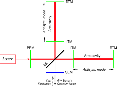
Figure 1: We draw a signal- (and power-) recycled LIGO interferometer. The laser light enters the interferometer from the left (bright port), through the power-recycling mirror (PRM), and gets split by a 50/50 beamsplitter into the two identical (in absence of gravitational waves) arm cavities. Each of the arm cavities is formed by the input test-mass (ITM) and the end test-mass (ETM) mirrors. A signal extracting mirror (SEM) is placed at the dark port, forming a signal extracting (SE) cavity with the ITMs.

This paper is organized as follows: in Section II we describe the modulation/demodulation process and derive the demodulated output of signal-recycled interferometers in terms of quadrature operators and arbitrary heterodyne field amplitudes — taking the simplest sine-wave modulation/demodulation scheme as an example; in Section III we derive the expressions of the quantum noise spectral density in this scheme, and apply them to initial and Advanced LIGO interferometers; in Section IV.1 we analyze a completely general modulation/demodulation scheme, derive a quantum limit for heterodyne measurements and discuss the consequence of this quantum limit for conventional interferometers. Finally, in Section V, we present our conclusions.

II The Radio-Frequency modulation-demodulation scheme in advanced LIGO

II.1 Overview of Advanced LIGO optical configuration

The Michelson interferometer is operated on the dark fringe to minimize static laser power, and hence the shot noise associated with this light, at the antisymmetric (dark) port. Since most of the light returns toward the laser, a partially transmitting mirror, the power-recycling mirror (PRM) is placed between the laser and the beam splitter to ‘recycle’ the light back into the interferometer Drever (see Fig. 1). The optical configuration currently planned to achieve quantum-limited performance in Advanced LIGO uses the Resonant Sideband Extraction (RSE) technique RSE , in addition to power-recycling. In RSE, an additional partially transmitting mirror, the signal extraction mirror (SEM), is placed between the antisymmetric port of the beamsplitter and photodetector (see Fig 1).

The optical properties (reflectivity, loss) of this signal extraction mirror and its microscopic position (in fractions of the wavelength of the laser light, $1.064\,\mu{\rm m}$) can significantly influence the frequency response of the interferometer SR ; RSE . When the signal extraction cavity (SEC) — comprising the SEM and the input test-mass (ITM) mirrors of the arm cavities — is exactly resonant or anti-resonant at the laser frequency, the bandwidth of the entire detector can be increased or decreased by altering the reflectivity of the SEM. These two special cases are referred to as resonant sideband extraction (RSE) RSE and signal recycling (SR) SR , respectively.

As the signal cavity is slightly offset (detuned) from resonance (RSE) or antiresonance (SR), the frequency at which the peak optical response of the detector occurs can be shifted to frequencies where other noise sources are not dominant. Note that, unlike conventional interferometers and tuned RSE/SR interferometers, the frequency responses of detuned configurations are no longer symmetric around the carrier frequency, with only one resonant peak located either higher or lower than the carrier frequency. As a consequence, although the interferometer will respond resonantly to GW’s with a certain nonzero frequency, only one of the two (upper and lower) sidebands the GW generates symmetrically around the carrier frequency is on resonance. More generally, the upper and lower GW sidebands contribute asymmetrically to the total output field, which makes the GW signal appear simultaneously in both quadratures of the output field BC1 ; BC2 ; BC3 ; BC4 . Detuned configurations are neither RSE nor SR in the original sense, but roughly speaking, such a configuration can be classified as either RSE or SR by looking at whether the bandwidth of the entire interferometer is broader or narrower than that of the arm cavity. Historically, since SR was invented earlier than RSE, some literature refers to all configurations with a signal mirror as “Signal Recycled”.

Since detuned RSE allows us to control the spectral response of the interferometer and optimize for specific astrophysical sources, it has become a strongly favored candidate for Advanced LIGO . A notable consequence is that with the high laser power of Advanced LIGO, the optomechanical coupling induced by detuned RSE/SR significantly modifies the dynamics of the interferometer, introducing an additional resonance at which the sensitivity also peaks BC1 ; BC2 ; BC3 ; BC4 .

II.2 Modulation and demodulation processes

The RF modulation-demodulation scheme comprises two parts: the modulation-preparation and demodulation-readout processes. In this section we consider only the simplest case, sine wave modulation and demodulation. A more general discussion of modulation/demodulation schemes can be found in Sec. IV.

Phase modulated light is incident on the interferometer. It is composed of the carrier at the laser frequency $\omega_{0}\sim 2\cdot 10^{15}\,{\rm s}^{-1}$, and a pair of phase modulation sidebands offset from the carrier by several MHz, so $\omega_{\rm m}\sim 2\pi\cdot 10^{6}\,{\rm s}^{-1}\gg$ GW-sideband frequency $<2\pi\cdot 10^{4}\,{\rm s}^{-1}$. The detection port is kept as dark as possible for the carrier, while the PM sidebands at $\omega_{0}\pm\omega_{\rm m}$ are coupled out as efficiently as possible to act as the local oscillator for the GW-induced carrier field that leaks out. Maximal RF sideband transmission is adjusted in two ways: (i) by a path difference in the arms of the Michelson that is arranged to be highly transmissive for the RF component of the field – the Schnupp asymmetry; and (ii) by matching the transmission of the power-recycling and signal-extracting mirrors so that the effective cavity comprising those two mirrors is critically coupled. In addition to the gravitational-wave readout, the PM sidebands are also useful for controlling the auxiliary degrees of freedom of the interferometer Srse02 .

In Fig. 2 we show the outgoing optical field at the interferometer output in the frequency domain, which consists of the GW sidebands, the Schnupp sidebands and quantum fluctuations at the output.

Figure 2: The outgoing field at the interferometer output consists of GW sideband signals around $\omega_{0}$, the Schnupp sideband fields at $\omega_{0}\pm\omega_{\rm m}$ and quantum fluctuations spread out at all frequencies.

The relative amplitudes of the RF sidebands are intentionally shown to be unequal. This is a case of unbalanced heterodyning, and is an intrinsic feature of the detuned RSE interferometer. As described above, when we move to detuned RSE, the SEC is detuned from perfect carrier resonance, such that the resonance peak of the signal cavity coincides with one of the GW signal sidebands, at the expense of the other one; consequently, the GW signal appears in both quadratures of the output field. At the same time, this phase shift in the signal cavity moves both RF sidebands off perfect resonance as well, which results in poor output coupling of both RF sidebands. This can be remedied by offsetting the RF sideband frequency – or conversely, the macroscopic length of the SEC – to make one of the RF sidebands resonant MW . Hence, detuned RSE leads to unbalanced heterodyne fields. Although the carrier is phase modulated before entering the interferometer, the heterodyne fields at the output port will no longer act as a pure phase modulation on the carrier.

At the detection port, a standard heterodyne detection procedure is used to extract the GW signal:

$${\rm Outgoing\;light}\Rightarrow{\rm Photodetection}\rightarrow{\rm Mixing\;with}\,\cos(\omega_{\rm m}t+\phi_{\rm D})\rightarrow{\rm Low-pass\;filter}\Rightarrow{\rm Demodulated\;output}$$

The photodetection process consists of taking the square of the optical field shown in Fig. 2. This operation mixes the GW signal (and quantum fluctuations) located at frequency $\sim\omega_{0}$ with the RF sideband fields located at frequency $\omega_{0}\pm\omega_{\rm m}$. As a consequence the GW signal is measured in the RF band around $\pm\omega_{\rm m}$. By taking the product of (or mixing) the photodetection output with the demodulation function, $\cos(\omega_{\rm m}t+\phi_{\rm D})$, the GW signal is down-converted back to low frequencies. The result is then filtered by a low-pass filter, yielding a frequency-independent quadrature that does depend on $\phi_{\rm D}$. However, as we shall see more quantitatively in the following sections, in addition to the GW signal (and quantum fluctuations) centered at $\sim\omega_{0}$, quantum fluctuations at $\sim\omega_{0}\pm 2\omega_{\rm m}$ also enter the demodulated output at the antisymmetric port. This gives rise to an additional noise term that is not present in a homodyne readout scheme.

II.3 Demodulated output of LIGO interferometers

The optical field coming out from the interferometer [see Fig. 1] can be written as a sum of two parts:

$${E}(t)=L(t)+{S}(t)\,.$$ (1)

The first term,

$$L(t)=\left[D_{+}e^{i\,(\omega_{0}+\omega_{\rm m})\,t}+D_{-}e^{i\,(\omega_{0}-\omega_{\rm m})\,t}\right]+{\rm h.c.}\,,$$ (2)

is the (classical) LO light composed of the Schnupp sideband fields at frequencies $\omega_{0}\pm\omega_{\rm m}$, with (complex) amplitudes $D_{+}$ and $D_{-}$, respectively. The magnitude and phase of $D_{\pm}$ depend on the specific optical configuration. The two quadratures of the LO are generated by either amplitude modulation (first quadrature) or phase modulation (second quadrature) of the input light. The second term in Eq. (1) ,

$${S}(t) \equiv \int_{0}^{+\infty}\frac{d\omega}{2\pi}\left[\,e^{-i\omega t}\,{b}_{\omega}+{\rm h.c.}\right]\,,$$ (3)

$$= \int_{-\Lambda}^{+\Lambda}\frac{d\Omega}{2\,\pi}\,\left[\,e^{-i\,(\omega_{0}-2\omega_{\rm m}+\Omega)\,t}\,{b}_{\omega_{0}-2\omega_{\rm m}+\Omega}+{\rm h.c.}\right]$$

$$+ \int_{-\Lambda}^{+\Lambda}\frac{d\Omega}{2\,\pi}\,\left[\,e^{-i\,(\omega_{0}+\Omega)\,t}\,{b}_{\omega_{0}+\Omega}+{\rm h.c.}\right]$$

$$+ \int_{-\Lambda}^{+\Lambda}\frac{d\Omega}{2\,\pi}\,\left[\,e^{-i\,(\omega_{0}+2\omega_{\rm m}+\Omega)\,t}\,{b}_{\omega_{0}+2\omega_{\rm m}+\Omega}+{\rm h.c.}\right]$$

$$+ ({\rm contributions\;at\;irrelevant\;frequency\;bands})\,,$$

contains both the (classical) GW signal and the quantum fluctuations of optical fields near $\omega_{0}$. Here $\Lambda\lesssim\omega_{\rm m}$ is the demodulation bandwidth . [For simplicity and clarity, we only write out explicitly the terms that will eventually contribute to the demodulated output.]

The photocurrent from the photodetector is proportional to the square of the optical field,

$$i(t)\propto{E}^{2}(t) = L^{2}(t)+2L(t)\,{S}(t)+{S}^{2}(t)\,,$$ (4)

$$= \left[{\rm contributions\;at\;frequencies\;}0,\,\pm 2\omega_{\rm m},\,\pm(2\omega_{0}\pm 2\omega_{\rm m}),\;{\rm from\;}L^{2}(t)\right]$$

$$+ 2D_{+}\left[\int_{-\Lambda}^{+\Lambda}\frac{d\Omega}{2\pi}e^{i(\omega_{\rm m}-\Omega)t}\,{b}_{\omega_{0}+\Omega}+\int_{-\Lambda}^{+\Lambda}\frac{d\Omega}{2\pi}e^{-i(\omega_{\rm m}+\Omega)t}\,{b}_{\omega_{0}+2\omega_{\rm m}+\Omega}\right]+{\rm h.c.}$$

$$+ 2D_{-}\left[\int_{-\Lambda}^{+\Lambda}\frac{d\Omega}{2\pi}e^{i(\omega_{\rm m}-\Omega)t}\,{b}_{\omega_{0}-2\omega_{\rm m}+\Omega}+\int_{-\Lambda}^{+\Lambda}\frac{d\Omega}{2\pi}e^{-i(\omega_{\rm m}+\Omega)t}\,{b}_{\omega_{0}+\Omega}\right]+{\rm h.c.}$$

$$+ \left[{\rm contributions\;at\;irrelevant\;frequency\;bands}\right]$$

$$+ \left[{\rm terms\;quadratic\;in\;}{b},\,{b}^{\dagger},\;{\rm from\;}S^{2}(t)\right]\,.$$

After taking the product of (or mixing) $i(t)$ with $\cos(\omega_{\rm m}t+\phi_{\rm D})$ and applying a low-pass filter with cutoff frequency $\Lambda$, we obtain the demodulated output

$$i(t)\cos(\omega_{\rm m}t+\phi_{\rm D})\stackrel{{\scriptstyle\rm Low-pass}}{{\Longrightarrow}}{O}(\phi_{\rm D};t) = \int_{-\Lambda}^{+\Lambda}\frac{d\Omega}{2\pi}\left[\left(D_{+}e^{-i\phi_{\rm D}}+D_{-}e^{i\phi_{\rm D}}\right)e^{-i\,\Omega\,t}\,b_{\omega_{0}+\Omega}+{\rm h.c.}\right]$$ (5)

$$+ \int_{-\Lambda}^{+\Lambda}\frac{d\Omega}{2\pi}\left[D_{+}e^{i\phi_{\rm D}}e^{-i\,\Omega\,t}\,{b}_{\omega_{0}+2\omega_{\rm m}+\Omega}+{\rm h.c.}\right]$$

$$+ \int_{-\Lambda}^{+\Lambda}\frac{d\Omega}{2\pi}\left[D_{-}e^{-i\phi_{\rm D}}e^{-i\,\Omega\,t}\,{b}_{\omega_{0}-2\omega_{\rm m}+\Omega}+{\rm h.c.}\right]\,,$$

where we assume the local oscillator to be strong enough that the quadratic terms in Eq. (4) can be ignored. It is convenient to recast the demodulated output (5) in terms of quadrature operators by using the following relation (for $\Lambda\ll\omega$):

$$\int_{-\Lambda}^{+\Lambda}\frac{d\Omega}{2\pi}\left[Ae^{-i\,\Omega\,t}\,{b}_{\omega+\Omega}+A^{*}e^{i\,\Omega\,t}\,{b}^{\dagger}_{\omega+\Omega}\right]=\int_{0}^{+\Lambda}\frac{d\Omega}{2\pi}\sqrt{2}\,A_{0}\,e^{-i\,\Omega\,t}\,{b}_{\alpha+\frac{\pi}{2}}^{\omega}(\Omega)+{\rm h.c.}\,.$$ (6)

Here $A=A_{0}\,e^{i\alpha}$ ($A_{0},\,\alpha\in\Re$) is an arbitrary complex amplitude, and the quadrature operator ${b}_{\alpha+\frac{\pi}{2}}^{\omega}$ is defined as [see also Refs. BC1 ; BC2 ]

$${b}_{\zeta}^{\omega}(\Omega)={b}_{1}^{\omega}(\Omega)\sin\zeta+{b}_{2}^{\omega}(\Omega)\cos\zeta\,,$$ (7)

where

$${b}_{1}^{\omega}(\Omega)=\frac{{b}_{\omega+\Omega}+{b}_{\omega-\Omega}^{\dagger}}{\sqrt{2}}\,,\quad\quad{b}_{2}^{\omega}(\Omega)=\frac{{b}_{\omega+\Omega}-{b}_{\omega-\Omega}^{\dagger}}{\sqrt{2}i}\,.$$ (8)

The superscript $\omega$ on the quadrature fields is added to emphasize that the quadratures are defined with respect to the central frequency $\omega$. By applying relation (6) to the demodulated output (5), we get

$${O}(\phi_{\rm D};t)=\int_{0}^{+\Lambda}\frac{d\Omega}{2\pi}e^{-i\,\Omega\,t}\sqrt{2}\left[D_{0}\,{b}_{\zeta_{0}}^{\omega_{0}}(\Omega)+\left|D_{+}\right|\,{b}_{\zeta_{+}}^{\omega_{0}+2\omega_{\rm m}}(\Omega)+\left|D_{-}\right|\,{b}_{\zeta_{-}}^{\omega_{0}-2\omega_{\rm m}}(\Omega)\right]+{\rm h.c.}\,,$$ (9)

in which we have defined,

$$D_{0}\equiv\left|D_{+}\,e^{-i\phi_{\rm D}}+D_{-}\,e^{i\phi_{\rm D}}\right|\,,$$ (10)

and

$$\zeta_{0} \equiv \frac{\pi}{2}+\arg\left(D_{+}\,e^{-i\phi_{\rm D}}+D_{-}\,e^{i\phi_{\rm D}}\right)\,,$$ (11)

$$\zeta_{\pm} \equiv \pm\phi_{\rm D}+\frac{\pi}{2}+\arg D_{\pm}\,.$$ (12)

In the frequency domain, we have,

$${O}(\phi_{\rm D};\Omega)=\sqrt{2}D_{0}\left[{b}_{\zeta_{0}}^{\omega_{0}}(\Omega)+\frac{\left|D_{+}\right|}{D_{0}}\,{b}_{\zeta_{+}}^{\omega_{0}+2\omega_{\rm m}}(\Omega)+\frac{\left|D_{-}\right|}{D_{0}}\,{b}_{\zeta_{-}}^{\omega_{0}-2\omega_{\rm m}}(\Omega)\right]\,,\quad\quad|\Omega|<\Lambda\,.$$ (13)

The first term inside the parenthesis, $b_{\zeta_{0}}^{\omega_{0}}$ is an output quadrature field around the carrier frequency $\omega_{0}$, which contains both the GW signal and vacuum fluctuations in the optical fields near the carrier frequency. In Refs. BC1 ; BC2 ; BC3 ; BC4 , this quadrature field is related to the input quadrature field at the antisymmetric port via the input-output relations, from which the spectral density of the quantum noise can be derived. Measuring this field is the task of all readout schemes. For example, a homodyne scheme can measure directly an arbitrary frequency-independent quadrature. For this reason, we call the quadrature field $b_{\zeta_{0}}^{\omega_{0}}$ the homodyne quadrature for distinction. The two additional terms inside the parenthesis are the additional noise, which come from vacuum fluctuations around $\omega_{0}\pm 2\omega_{m}$. The sum of all three terms is what we measure in the heterodyne scheme, which we call the heterodyne quadrature.

Quantity	Symbol and Value
Laser frequency	$\omega_{0}=1.8\times 10^{15}\,{\rm sec}^{-1}$
GW sideband frequency	$\Omega$
Input test-mass transmissivity	$T$
Arm-cavity length	$L=4\,{\rm km}$
Mirror mass	$m$
Light power at beamsplitter	$I_{0}$
SEM amplitude reflectivity and transmissivity	$\rho,\tau$
SEC length	$l\sim 10\,{\rm m}$
SEC detuning	$\phi=[\omega_{0}l/c]_{\rm mod\,2\pi}$

Table 1: Basic quantities of Advanced LIGO interferometers

II.4 Features of the RF modulation-demodulation scheme

As can be inferred from Eq. (11), as long as $|D_{+}|\neq|D_{-}|$, all homodyne quadratures can be measured through some heterodyne quadrature with the appropriate demodulation phase $\phi_{\rm D}$. The (single-sided) spectral density $S(\Omega)$ associated with the noise $h_{n}$ can be computed by the formula [see Eq. (22) of Ref. KLMTV00 ]:

$$2\pi\,\delta(\Omega-\Omega^{\prime})\,S(\Omega)=\langle{\rm in}|h_{n}(\Omega)\,h_{n}^{\dagger}(\Omega^{\prime})+h_{n}^{\dagger}(\Omega^{\prime})\,h_{n}(\Omega)|{\rm in}\rangle\,,$$ (14)

and if the input state of the whole interferometer is the vacuum state ($|{\rm in}\rangle=|0_{{a}}\rangle$), the following relation holds:

$$\langle 0_{{a}}|{a}_{i}(\Omega)\,{a}^{\dagger}_{j}(\Omega^{\prime})+{a}^{\dagger}_{j}(\Omega^{\prime})\,{a}_{i}(\Omega)|0_{{a}}\rangle=2\pi\,\delta(\Omega-\Omega^{\prime})\,\delta_{ij}\,.$$ (15)

From Eq. (13) we see that the noise spectral density in the heterodyne quadrature is a sum of that of the homodyne quadrature, $S_{b}^{\rm hom}(\phi_{\rm D};\Omega)$, and those of the additional noise terms, $S_{b}^{\rm add}(\phi_{\rm D};\Omega)$. Since $S_{b}^{\rm hom}(\phi_{\rm D};\Omega)$ and $S_{b}^{\rm add}(\phi_{\rm D};\Omega)$ come from different frequency bands, we assume that they are uncorrelated, hence

$$S_{b}^{\rm het}(\phi_{\rm D};\Omega)=S_{b}^{\rm hom}(\phi_{\rm D};\Omega)+S_{b}^{\rm add}(\phi_{\rm D};\Omega)\,.$$ (16)

Assuming that the fields associated with the additional heterodyne noise are in the vacuum state, we get a white (frequency-independent) spectrum for the additional noise,

$$S_{b}^{\rm add}(\phi_{\rm D})=\frac{|D_{+}|^{2}+|D_{-}|^{2}}{D_{0}^{2}}=\frac{|D_{+}|^{2}+|D_{-}|^{2}}{|D_{+}e^{-i\phi_{\rm D}}+D_{-}e^{i\phi_{\rm D}}|^{2}}\,,$$ (17)

which usually depends on $\phi_{\rm D}$, unless either $D_{+}$ or $D_{-}$ is zero, which we refer to as the totally unbalanced case. In the case of balanced modulation, when $|D_{+}|=|D_{-}|$, only one quadrature,

$$\zeta_{0}^{\rm balanced}=\frac{\pi}{2}+\frac{1}{2}\left(\arg D_{+}+\arg D_{-}\right)\,,$$ (18)

is measured, with additional noise

$$S_{b}^{\rm add\,balanced}=\frac{1}{2}\,,$$ (19)

and with a frequency-independent optimal demodulation phase

$$\phi_{\rm D}^{\rm balanced}=\frac{1}{2}\left[\arg D_{+}-\arg D_{-}\right]+N\pi\,,\quad N=0,\,\pm 1,\,\ldots.$$ (20)

This is the lowest possible additional noise for heterodyne schemes with just one pair of sidebands. The noise spectral density can have different shapes as a function of the homodyne angle KLMTV00 ; BC1 . At different signal sideband frequencies, the optimal homodyne angle $\zeta_{\rm opt}$ that gives the lowest homodyne noise can be different. In homodyne detection, since both quadratures of the carrier are generally not available, only a single frequency-independent quadrature can be measured . By contrast, in heterodyne detection schemes (except for the balanced case), all quadratures are available for simultaneous measurement, and the final heterodyne noise at each frequency will be the minimum of all quadratures.

III Noise spectral density and the effect of the additional noise

In this section, we write down the noise spectral density for both conventional and RSE interferometers when the RF modulation-demodulation scheme described in Section II is used.

Symbol	Quantity	Expression
$\gamma$	Half bandwidth of arm cavity	$\displaystyle\frac{Tc}{4L}$
$\beta$	Phase gained by resonant field in arm cavity	$\arctan(\Omega/\gamma)$
$h_{\rm SQL}$	Free-mass standard quantum limit	$\displaystyle\sqrt{\frac{8\hbar}{m\Omega^{2}L^{2}}}$
$I_{\rm SQL}$	Characteristic input power for conventional interferometer to reach the SQL at $\Omega=\gamma$	$\displaystyle\frac{mL^{2}\gamma^{4}}{4\omega_{0}}$
$\cal K$	Coupling constant for radiation-pressure effects	$\displaystyle\frac{2(I_{0}/I_{\rm SQL})\gamma^{4}}{\Omega^{2}(\Omega^{2}+\gamma^{2})}$

Table 2: Quantities derived from those listed in Tab. 1

III.1 Total noise spectral density

The input-output relation for RSE interferometers, including optomechanical effects, were derived in Refs. BC1 ; BC2 [see Eqs. (2.20)–(2.24) and (2.26) of Ref. BC2 ]. The output fields in the frequency band of $(\omega_{0}-\Lambda,\,\omega_{0}+\Lambda)$ are (in the conventions used in this manuscript)

$$\left(\matrix{{b}_{1}^{\omega_{0}}\cr{b}_{2}^{\omega_{0}}}\right)=\frac{1}{M}\left[e^{2i\beta}\left(\matrix{C_{11}&C_{12}\cr C_{21}&C_{22}}\right)\left(\matrix{{a}_{1}^{\omega_{0}}\cr{a}_{2}^{\omega_{0}}}\right)+\sqrt{2{\cal K}}\tau e^{i\beta}\left(\matrix{D_{1}\cr D_{2}}\right)\frac{h}{h_{\rm SQL}}\right]\,,$$ (21)

where

$$M=1+\rho^{2}\,e^{4i\beta}-2\rho\,e^{2i\beta}\left(\cos{2\phi}+\frac{{\cal K}}{2}\,\sin{2\phi}\right)\,,$$ (22)

$$C_{11}=C_{22}=(1+\rho^{2})\,\left(\cos{2\phi}+\frac{{\cal K}}{2}\,\sin{2\phi}\right)-2\rho\,\cos{2\beta}\,,$$ (23)

$$C_{12}=-\tau^{2}\,(\sin{2\phi}+{\cal K}\,\sin^{2}{\phi})\,,\quad\quad C_{21}=\tau^{2}\,(\sin{2\phi}-{\cal K}\,\cos^{2}{\phi})\,,$$ (24)

$$D_{1}=-(1+\rho\,e^{2i\beta})\,\sin{\phi}\,,\quad\quad D_{2}=-(-1+\rho\,e^{2i\beta})\,\cos{\phi}\,.$$ (25)

The quantities $\cal K$, $\beta$, $\rho$, $\phi$, $\tau$ and $h_{\rm SQL}$ are defined in the same way as in Refs. BC1 ; BC2 ; BC3 . We denote by $h(\Omega)$ the gravitational strain and give a summary of the main quantities in Tables 1 and 2. We assume that the fields $a^{\omega_{0}}$ incident on the unused input of the antisymmetric port are in the vacuum state for all frequencies. Moreover, the additional heterodyne noise fields $b^{\omega_{0}\pm 2\omega_{m}}$ in Eq. (13) must also be in vacuum states, since they are far away from the carrier frequency and are not affected by the ponderomotive squeezing effects of the interferometer. We assume that the higher-order terms of the modulation are not resonant in the interferometer, which is in general the case. Even if the higher-order sidebands are resonance, we would not expect any ponderomotive squeezing since the frequency is too high for the test-mass displacement to respond to an external force. Using Eqs. (14)–(17) and (21), we obtain the total heterodyne noise spectral density in $h$, as a sum of the corresponding homodyne noise (first term) and the additional heterodyne noise (second term) [see Eqs. (10), (11) for the definitions of $D_{0}$ and $\zeta_{0}$]:

$$S_{h}^{\rm het}(\phi_{\rm D};\Omega) = \frac{h_{\rm SQL}^{2}}{2{\cal K}}\,\frac{1}{\tau^{2}\,\left|D_{1}\,\sin\zeta_{0}+D_{2}\,\cos\zeta_{0}\right|^{2}}\,\left[{\left(C_{11}\,\sin\zeta_{0}+C_{21}\,\cos\zeta_{0}\right)^{2}+\left(C_{12}\,\sin\zeta_{0}+C_{22}\,\cos\zeta_{0}\right)^{2}}\right]+$$ (26)

$$\frac{h_{\rm SQL}^{2}}{2{\cal K}}\,\frac{1}{\tau^{2}\,\left|D_{1}\,\sin\zeta_{0}+D_{2}\,\cos\zeta_{0}\right|^{2}}\,\left[\frac{\left|D_{+}\right|^{2}+\left|D_{-}\right|^{2}}{\left|D_{+}\,e^{-i\phi_{\rm D}}+D_{-}\,e^{i\phi_{\rm D}}\right|^{2}}\left|M\right|^{2}\right]\,.$$

We note that the optimal heterodyne noise spectral density at a given GW signal sideband frequency is the minimum of those obtained varying $\phi_{\rm D}$ (and thus $\zeta_{0}$).

III.2 Conventional interferometers

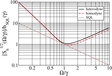
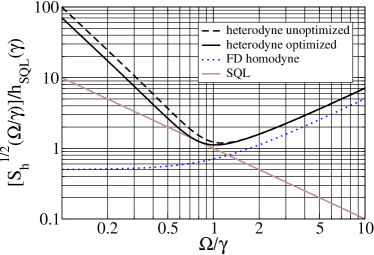
Figure 3: In the left panel we show the square root of noise spectral density, in units of $h_{\rm SQL}(\gamma)$, for a conventional interferometer with $I_{0}=I_{\rm SQL}$, using balanced heterodyne modulation (solid curve) and the homodyne (dashed curve) scheme, plotted as functions of $\Omega/\gamma$. The second quadrature is measured. In the right panel we plot the noise spectral density of the same interferometer, using unbalanced heterodyne detection, with homodyne angle chosen at the optimal value for the homodyne case, $\zeta(\Omega)=\zeta_{\rm opt\,hom}(\Omega)$ (dashed line), and at the re-optimized value for the heterodyne case $\zeta(\Omega)=\zeta_{\rm opt\,het}(\Omega)$ (solid curve), respectively. The optimal heterodyne noise spectral density without the additional noise is also shown (dotted curve), which agrees with the result for frequency-independent homodyne detection  KLMTV00 . The SQL line is shown in both panels as gray straight lines.

For the power-recycled Fabry-Perot Michelson optical configuration, the so-called conventional interferometer, the GW signal appears only in the second (or phase) quadrature. Furthermore, barring imperfections, the transmission of the Schnupp sidebands is balanced. In our notation such a scheme is obtained by setting $D_{-}=-D_{+}^{*}$, with $\phi_{\rm D}=\pm\pi/2+\arg D_{+}$ which is the optimal demodulation phase for all frequencies [see Eq. (20)]. Evaluating Eq. (26) in the case $\phi=0,\tau=1$, we get

$$S_{h}^{\rm het\,\mbox{\scriptsize conv}}=\frac{h_{\rm SQL}^{2}}{2{\cal K}}\left({\cal K}^{2}+1+\frac{1}{2}\right)\,,$$ (27)

where the last term inside the parenthesis is the additional heterodyne noise, which is equal to $1/2$ the shot noise in homodyne readout scheme (second term), originally derived in Ref. MS91 . In the left panel of Fig. 3, we plot the noise curves of a conventional interferometer with $I_{0}=I_{\rm SQL}$, using homodyne and balanced heterodyne detection, respectively, with the second quadrature measured. This is exactly the result in Ref. N88 . More sophisticated modulation schemes that can further lower or eliminate the additional heterodyne noise in this quadrature have been investigated by Schnupp Schnupp , Niebauer et al. N88 , and Meers and Strain MS91 .

If, on the contrary, the RF sidebands at the antisymmetric port are not balanced, one can measure arbitrary quadratures by adjusting the demodulation phase [see Sec. II.4]. As proposed by Vyatchanin, Matsko and Zubova  VMZ , and further investigated by Kimble, Levin, Matsko, Thorne and Vyatchanin (KLMTV) KLMTV00 , measuring different quadratures at different GW signal sideband frequencies can allow conventional interferometers to beat the Standard Quantum Limit (SQL) SQL significantly, thus converting them into a QND interferometer. Somiya Somiya proposed that, by using a frequency-dependent demodulation phase, a KLMTV-type, frequency-dependent optimization is achievable in a totally unbalanced modulation scheme. However, the effect of the additional heterodyne noise was not explicitly taken into account and we show in this section that the additional heterodyne noise plays an important role as soon as one approaches the SQL. So much so, that for totally unbalanced heterodyne detection, the SQL cannot be beaten, and for intermediate levels of imbalance the SQL is beaten by very modest amounts.

For simplicity, we first consider a totally unbalanced modulation scheme (which was the case investigated by Somiya Somiya ), in which only $D_{+}$ (or only $D_{-}$) is non-zero. From Eq. (26), fixing $\tau=1$, $\rho=0$ and $\phi=0$, we have

$$S_{h}^{\rm het\,conv}=\frac{h_{\rm SQL}^{2}}{2{\cal K}}\left[({\cal K}-\tan\zeta_{0})^{2}+1+\frac{1}{\cos^{2}\zeta_{0}}\right]\,,$$ (28)

where the last term inside the parenthesis is the additional noise due to heterodyne detection. Using the optimal detection angle in the (frequency dependent) homodyne case VMZ ; KLMTV00 , $\zeta_{\rm opt\,hom}=\arctan{\cal K}$, one has

$$S_{h}=\frac{h_{\rm SQL}^{2}}{2{\cal K}}\left({\cal K}^{2}+2\right)\geq\sqrt{2}h_{\rm SQL}^{2}\,,$$ (29)

which cannot reach the SQL. Re-optimizing the detection angle, we obtain $\zeta_{\rm opt\,het}=\arctan({\cal K}/2)$. This gives

$$\left[S_{h}^{\rm het\,conv}\right]_{\rm opt}=\frac{h_{\rm SQL}^{2}}{2{\cal K}}\left(\frac{{\cal K}^{2}}{2}+2\right)\geq h_{\rm SQL}^{2}\,,$$ (30)

which only touches, but never beats, the SQL. In the right panel of Fig. 3, we plot the noise curve of a conventional interferometer with $I_{0}=I_{\rm SQL}$, the heterodyne noise spectral density using $\zeta_{\rm opt\,hom}$ [given by Eq. (29)], and the optimal heterodyne noise spectral density [given by Eq. (30)]. As can be further verified, having two sidebands with unequal amplitude can allow the interferometer to beat the SQL, but only by very moderate amounts, and in limited frequency bands.

We might still expect to use more sophisticated modulation-demodulation schemes to lower the additional heterodyne noise while retaining the possibility of variable-quadrature optimization. However, as we shall see in Sec. IV, such an effort will be significantly limited by the Heisenberg uncertainty principle.

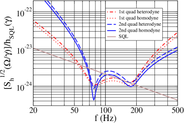
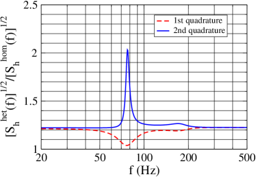
Figure 4: A detuned RSE interferometer ($T=0.033$, $\rho=0.9$, $\phi=\pi/2-0.47$, $m=30\,{\rm kg}$, $I_{0}=I_{\rm SQL}$) using balanced heterodyne detection. In the left panel we plot the square root of total heterodyne noise spectral density in the first (dash-dot curve) and second (long dashed curve) quadratures, compared with the homodyne ones (dot curve and solid curve, respectively). The SQL line is also shown as a gray straight line. In the right panel we show the ratio of the square roots of the heterodyne and the homodyne noise spectral densities, for the first (dashed curve) and second (solid curve) quadratures.

III.3 Signal-recycled interferometers

In this section, we give some examples of noise curves of detuned RSE interferometers with a heterodyne readout scheme, and compare them to the homodyne cases.

In the balanced scheme the additional heterodyne noise is the lowest, but only one quadrature can be measured. For this case we show the effect of the additional heterodyne noise on the sensitivity curves in Fig. 4. In the left panel, we plot the noise curves for a detuned RSE interferometer with $T=0.033$, $\rho=0.9$, $\phi=\pi/2-0.47$, $I_{0}=I_{\rm SQL}$ and $m=30\,{\rm kg}$, (the configuration considered in Refs. BC1 ; BC2 ; BC3 ) when the first ($\zeta=\pi/2$) and second quadratures ($\zeta=0$) are measured, by homodyne and balanced heterodyne read-out schemes. In the right panel, we plot the ratio of the heterodyne noise to the corresponding homodyne ones. The additional heterodyne noise has more features around the two valleys of the noise curves, where the optomechanical dynamics (the RSE transfer function) determines the shape of the curves. Above $\sim 200$ Hz, the ratio between the square roots of the heterodyne and the homodyne noise spectral densities assumes the constant value $\sqrt{3/2}\sim 1.22$, which is due to the additional heterodyne noise when the shot noise dominates [see Eq. (27)].

Practical implementation of the RF sidebands in the interferometer has shown that detuned RSE configurations are likely to be very unbalanced MW ; BCM2 . In the left panel of Fig. 5, we plot the unbalanced heterodyne noise spectral densities for the same interferometer parameters used in Fig. 4, with $\zeta_{0}=0$, $\pi/4$, $\pi/2$ and $3\pi/4$, and the optimal heterodyne noise obtained by maximizing over $\zeta_{0}$ at each sideband frequency. Indeed, in the heterodyne readout scheme we have the advantage of optimizing the detection angle at different frequencies. At each particular signal sideband frequency, the optimal heterodyne noise spectral density is just the minimum of all quadratures. In the right panel of Fig. 5, we compare the optimal heterodyne noise with the homodyne noise at $\zeta=0$ and $\zeta=\pi/2$. As we see from this example, for the same interferometer configuration, neither the homodyne nor the heterodyne readout can provide a noise spectral density that is the lowest for all GW signal sideband frequencies. To make a more rigorous comparison between these two schemes a more critical study is required that takes into consideration specific astrophysical GW sources, the experimental feasibility and the other sources of noise, as well. [As an example, current Advanced LIGO design estimates the dominant, thermoelastic component at about the SQL therm . To lower the thermoelastic contribution below the SQL an interesting and challenging proposal has been analyzed recently DOSTVB .] The optimization of homodyne versus heterodyne readout schemes which include those effects is currently underway, and will be reported elsewhere BCM2 .

As shown in Ref. BC3 , detuned RSE interferometers have an unstable optomechanical resonance. In the parameter regime emphasized in Refs. BC1 ; BC2 ; BC3 ; BC4 , the unstable resonance lies within the observation band — which gives a dip in the noise spectrum. Consequently, the control scheme must sense and act on the motion of the system within the observation band. In Ref. BC3 , an idealized control scheme is conceived for the homodyne readout, which suppresses the instability and leaves the noise spectral density unchanged. The same control issue will need to be addressed with the heterodyne readout scheme as well.

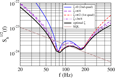
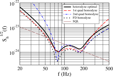
Figure 5: A detuned RSE interferometer ($T=0.033$, $\rho=0.9$, $\phi=\pi/2-0.47$, $m=30\,{\rm kg}$, $I_{0}=I_{\rm SQL}$, same as Fig. 4) using totally unbalanced heterodyne detection. In the left panel we show the noise curves for quadratures with $\zeta=0$ (solid curve), $\pi/4$ (long dashed curve), $\pi/2$ (short dashed curve) and $3\pi/4$ (dash-dot curve) are shown, together with the final heterodyne noise optimized at all sideband frequencies (thick solid curve). In the right panel, the final heterodyne noise (thick solid curve) is shown along with the homodyne noise in the first (dashed curve) and second (dash-dot curve) quadratures. The optimal heterodyne noise without the additional noise is also shown (dotted curve) for comparison. The SQL is plotted in both panels as gray straight lines.

IV More general discussion of heterodyne schemes: minimal additional noise and quantum limit

In Sec. II we discussed the sinusoidal modulation-demodulation scheme, which is the easiest to implement. There exist more sophisticated schemes, such as those proposed by Schnupp, investigated by Niebauer et al. N88 , and Meers and Strain MS91 , that can further optimize the interferometer performances. These authors restricted their analyses to low-power interferometers and focused on the detection of the second (or phase) quadrature. In this section, we extend their discussions to the more general case where all quadratures can be measured. As we shall see, although modulation/demodulation readout schemes offers the advantage of variable-quadrature optimization, they are in general limited in converting non-QND interferometers to (broadband) QND interferometers.

IV.1 Quantum Limit for the additional heterodyne noise

The field coming out from the dark port can be written, in time domain, as

$$E(t)=\left[A(t)\cos\omega_{0}t+P(t)\sin\omega_{0}t\right]+\left[E_{1}(t)\cos\omega_{0}t+E_{2}(t)\sin\omega_{0}t\right]\,,$$ (31)

where the first term is the transmitted Schnupp sideband fields in the form of a combination of amplitude modulation [$A(t)$] and phase modulation [$P(t)$] to the carrier. In Eq. (31) we denoted by $E_{1}(t)$ and $E_{2}(t)$ the quadrature fields containing GW signal and quantum fluctuations. The output from the photodetector is then

$$i(t)\propto A(t)E_{1}(t)+P(t)E_{2}(t)\,.$$ (32)

The amplitude and phase modulation is in general periodic functions, with the same angular frequency $\omega_{\rm m}$ [$\omega_{0}\gg\omega_{\rm m}\gg\Omega_{\rm GW}$]:

$$A(t) = \sum_{k}A_{k}e^{-ik\omega_{m}t}\,,\quad A_{k}=A^{*}_{-k}\,;$$ (33)

$$P(t) = \sum_{k}P_{k}e^{-ik\omega_{m}t}\,,\quad P_{k}=P^{*}_{-k}\,.$$ (34)

In the frequency domain Eq. (32) reads:

$$i(\Omega)\propto\sum_{k}\left[A_{k}b_{1}^{\omega_{0}}(\Omega-k\omega_{\rm m})+P_{k}b_{2}^{\omega_{0}}(\Omega-k\omega_{\rm m})\right]\,.$$ (36)

Denoting the demodulation function with $D(t)$, the demodulated output is:

$$O(t)=D(t)i(t)\propto D(t)A(t)E_{1}(t)+D(t)P(t)E_{2}(t)\,.$$ (37)

The demodulation function $D(t)$ should have the same frequency as the modulation functions, therefore:

$$D(t)=\sum_{k}D_{k}e^{-ik\omega_{m}t}\,,\quad D_{k}=D^{*}_{-k}\,.$$ (38)

Note that Eq. (37) is a generalization of Eq. (4) of Ref. MS91 . Using the above equations, the Fourier transform of the demodulated output (37) can be written as:

$$\widetilde{O}(\Omega)=\sum_{k}D_{k}^{*}\left[A_{k}b_{1}^{\omega_{0}}(\Omega)+P_{k}b_{2}^{\omega_{0}}(\Omega)\right]+\sum_{p\neq 0}\sum_{k}D_{k}^{*}\left[A_{k+p}b_{1}^{\omega_{0}}(\Omega-p\,\omega_{m})+P_{k+p}b_{2}^{\omega_{0}}(\Omega-p\,\omega_{m})\right]\,.$$ (39)

Let us suppose that the low-frequency component of $\widetilde{O}(\Omega)$ is filtered out, then the first term in Eq. (39) gives a frequency-independent quadrature field near $\omega_{0}$, while the second term gives the additional heterodyne noise that arises from quantum fluctuations near $\omega_{0}\pm p\,\omega_{\rm m}$, with $p=\pm 1$, $\pm 2$, $\pm 3$, …. Since $\omega_{\rm m}\gg\Omega_{\rm GW}$, these fields are not affected by ponderomotive squeezing effects in the interferometer arm cavities and will be in the vacuum state. As a consequence, the additional heterodyne noise will also be frequency independent. [Unless frequency-dependent squeezed states are injected into the dark port of the interferometer.] In this way, for any particular quadrature $\zeta$, there is a uniform minimum of the additional heterodyne noise at all frequencies.

Let us now construct for an arbitrary quadrature $\zeta$ the optimal demodulation function $D(t)$ and evaluate the minimal additional noise. If we want to measure $b^{\omega_{0}}_{\zeta}$, Eq. (39) says that we have to impose

$$\left(\sum_{k}D_{k}^{*}A_{k},\sum_{k}D_{k}^{*}P_{k}\right)=(\sin\zeta,\cos\zeta)\,,$$ (40)

or in the time domain,

$$(\sin\zeta,\cos\zeta)=\left(\frac{1}{T}\int_{0}^{T}D(t)A(t)dt,\frac{1}{T}\int_{0}^{T}D(t)P(t)dt\right)\,,$$ (41)

where $T=2\pi/\omega_{\rm m}$ is the common period of the modulation and demodulation functions. Note that, in order for the quadrature $\zeta$ to be measured, Eqs. (40) and (41) need only be true up to a constant factor. Having written them in the current way, we have in fact chosen a specific normalization for $D(t)$. Using the Parseval theorem and Eq. (41), we derive for the spectral density of the additional heterodyne noise:

$$S^{\rm add} = \sum_{p\neq 0}\left|\sum_{k}D^{*}_{k}A_{k+p}\right|^{2}+\sum_{p\neq 0}\left|\sum_{k}D^{*}_{k}P_{k+p}\right|^{2}\,,$$ (42)

$$= \sum_{p}\left|\sum_{k}D^{*}_{k}A_{k+p}\right|^{2}+\sum_{p}\left|\sum_{k}D^{*}_{k}P_{k+p}\right|^{2}-\left|\sum_{k}D^{*}_{k}A_{k}\right|^{2}-\left|\sum_{k}D^{*}_{k}P_{k}\right|^{2}\,,$$

$$= \frac{1}{T}\int_{0}^{T}D^{2}(t)\left[A^{2}(t)+P^{2}(t)\right]dt-\left(\frac{1}{T}\int_{0}^{T}D(t)A(t)dt\right)^{2}-\left(\frac{1}{T}\int_{0}^{T}D(t)P(t)dt\right)^{2}\,,$$

$$= \frac{1}{T}\int_{0}^{T}D^{2}(t)\left[A^{2}(t)+P^{2}(t)\right]dt-1\,.$$

[Note that Eq. (42), which corresponds directly to Eq. (12) of Ref. MS91 , is also consistent with Eq. (18) of Ref. MS91 , since Eqs. (40) and (41) have already imposed a normalization for $D(t)$.] In order to find the $D(t)$ that satisfies Eq. (41) and minimize $S^{\rm add}$, we introduce two Lagrange multipliers, $\lambda$ and $\mu$, and impose,

$$\delta\int dt\Bigg{\{}\left[(A^{2}(t)+P^{2}(t)\right]D^{2}(t)-2\lambda A(t)D(t)-2\mu P(t)D(t)\Bigg{\}}=0\,,$$ (43)

which yields:

$$D(t)=\frac{\lambda A(t)+\mu P(t)}{A^{2}(t)+P^{2}(t)}\,.$$ (44)

[In Eq. (43), the factors of 2 in front of $\lambda$ and $\mu$ are added for simplicity.] Inserting Eq. (44) back into Eq. (41) gives,

$${\bf M}\left(\begin{array}[]{c}\lambda\\ \mu\end{array}\right)=\left(\begin{array}[]{c}\sin\zeta\\ \cos\zeta\end{array}\right)\,,$$ (45)

where

$${\bf M}=\left(\begin{array}[]{cc}\displaystyle\frac{1}{T}\int_{0}^{T}\frac{A^{2}(t)}{A^{2}(t)+P^{2}(t)}dt&\displaystyle\frac{1}{T}\int_{0}^{T}\frac{A(t)P(t)}{A^{2}(t)+P^{2}(t)}dt\\ \displaystyle\frac{1}{T}\int_{0}^{T}\frac{A(t)P(t)}{A^{2}(t)+P^{2}(t)}dt&\displaystyle\frac{1}{T}\int_{0}^{T}\frac{P^{2}(t)}{A^{2}(t)+P^{2}(t)}dt\end{array}\right)\,.$$ (46)

The optimal demodulation function for the $\zeta$ quadrature is then given by inverting Eq. (45) and inserting the resulting $\lambda$ and $\mu$ into Eq. (44). The minimal additional noise can be then obtained by inserting the optimal demodulation function into Eq. (42):

$$S^{\rm add\,min}(\zeta)=\left(\begin{array}[]{cc}\lambda&\mu\end{array}\right){\bf M}\left(\begin{array}[]{c}\lambda\\ \mu\end{array}\right)-1=\left(\begin{array}[]{cc}\sin\zeta&\cos\zeta\end{array}\right){\bf M}^{-1}\left(\begin{array}[]{c}\sin\zeta\\ \cos\zeta\end{array}\right)-1=\left(\begin{array}[]{cc}\sin\zeta&\cos\zeta\end{array}\right)\left({\bf M}^{-1}-{\bf I}\right)\left(\begin{array}[]{c}\sin\zeta\\ \cos\zeta\end{array}\right)\,.$$ (47)

Moreover, we note an interesting property of ${\bf M}$:

$${\bf I}-{\bf M}=(\det{\bf M}){\bf M}^{-1}\,.$$ (48)

As a consequence,

$${\bf M}^{-1}-{\bf I}={\bf M}^{-1}({\bf I}-{\bf M})=(\det{\bf M})({\bf M}^{-1})^{2},$$ (49)

so

$$\det\left[{\bf M}^{-1}-{\bf I}\right]=1\,.$$ (50)

This implies that, the minimal additional noise can be written in a form

$$S^{\rm add\,min}(\zeta)=\left(\begin{array}[]{cc}\sin\zeta&\cos\zeta\end{array}\right)\left(\begin{array}[]{rr}\cos\phi&\sin\phi\\ -\sin\phi&\cos\phi\end{array}\right)\left(\begin{array}[]{cc}e^{R}&\\ &e^{-R}\end{array}\right)\left(\begin{array}[]{rr}\cos\phi&-\sin\phi\\ \sin\phi&\cos\phi\end{array}\right)\left(\begin{array}[]{c}\sin\zeta\\ \cos\zeta\end{array}\right)\,,$$ (51)

with $\phi$ and $R$ frequency-independent, and determined by the eigenvectors and eigenvalues of the matrix ${\bf M}^{-1}-{\bf 1}$, which are determined ultimately by the amplitude and phase modulations. It is interesting to note that this minimal noise spectrum is of exactly the same form as that of a squeezed state.

This phenomenon could in fact be anticipated from quantum mechanics. For the same sideband frequency $\Omega$, the different quadratures do not commute with each other, and have the following commutation relations:

$$\left[b^{\omega_{0}}_{\zeta}(\Omega),b^{\omega_{0}\,\dagger}_{\zeta^{\prime}}(\Omega^{\prime})\right]=2\pi i\sin(\zeta-\zeta^{\prime})\delta(\Omega-\Omega^{\prime})\,.$$ (52)

As a consequence, quantum fluctuations in the various quadratures are constrained by the Heisenberg uncertainty principle. As is well known, the squeezed states have the minimum noise spectrum allowed by the uncertainty principle. In modulation/demodulation schemes, all quadratures can be read out, with additional noise:

$$b^{\rm het}(\zeta,\Omega)=b^{\omega_{0}}_{\zeta}(\Omega)+n(\zeta,\Omega)\,.$$ (53)

So, all output observables should commute with each other, and as a consequence

$$\left[b^{\rm het}(\zeta,\Omega),b^{\rm het\dagger}(\zeta^{\prime},\Omega^{\prime})\right]=0\,.$$ (54)

Since $b^{\omega_{0}}_{\zeta}(\Omega)$ and $n(\zeta,\Omega)$ come from different frequency bands of the output field, they must commute with each other, so we must have that the mutual commutators of $n(\zeta,\Omega)$ cancel those of $b^{\omega_{0}}_{\zeta}(\Omega)$:

$$\left[n(\zeta,\Omega),n^{\dagger}(\zeta^{\prime},\Omega^{\prime})\right]=-2\pi i\sin(\zeta-\zeta^{\prime})\delta(\Omega-\Omega^{\prime})\,.$$ (55)

Since they do not commute with each other, the additional noise $n(\zeta,\Omega)$ is also subject to the constraint of the Heisenberg uncertainty principle — in the same way as $b^{\omega_{0}}_{\zeta}(\Omega)$, since the commutators only differ by a sign [see Eqs. (52) and (55)]. This explains why the minimum additional heterodyne noise has a spectral density of the same form as the squeezed states. The minimum noise spectrum (51) can be regarded as a quantum limit for modulation/demodulation schemes.

IV.2 Impact of the Quantum Limit on conventional interferometers

As discussed in Refs. VMZ ; KLMTV00 , using an appropriate readout scheme, conventional interferometers can achieve QND performance through a cancellation between shot and radiation-pressure noises. If the quadrature $\zeta$ is measured, we have

$$b^{\rm het\,conv}(\zeta,\Omega)=\cos\zeta\left[e^{2i\beta}\left(\tan\zeta-\mathcal{K}\right)a_{1}^{\omega_{0}}+e^{2i\beta}a_{2}^{\omega_{0}}+e^{i\beta}\sqrt{2\mathcal{K}}\frac{h}{h_{\rm SQL}}\right]+n(\zeta,\Omega)\,,$$ (56)

and if we choose to measure the quadrature with $\zeta=\zeta_{\rm c}=\arctan\mathcal{K}$ the part of the shot noise [the term proportional to $a_{1}^{\omega_{0}}\tan\zeta$ inside the bracket of Eq. (56)] cancels the radiation-pressure noise [the term proportional to $\mathcal{K}a_{1}^{\omega_{0}}$ inside the bracket of Eq. (56)]. The remaining shot noise [obtained from the term proportional to $a_{2}^{\omega_{0}}$ inside the bracket of Eq. (56)], normalized to unit signal strength, is inversely proportional to $\mathcal{K}$, and it can be made lower (eventually lower than the SQL noise) by taking larger $\mathcal{K}$. However, for larger values of $\mathcal{K}$, $\tan\zeta_{\rm c}$ grows and the corresponding $\cos\zeta_{\rm c}$ decreases. As can be seen from Eq. (56), this implies an even smaller signal strength in the detected quadrature, which makes the additional noise, $n(\zeta_{\rm c},\Omega)$, more and more important. In fact, more generally the additional noise limits the extent to which the interferometer can beat the SQL. Writing the total heterodyne noise spectral density [of which Eq. (28) is a special case], as

$$S_{h}=\frac{h_{\rm SQL}^{2}}{2\,\mathcal{K}}\left[(\mathcal{K}-\tan\zeta)^{2}+1+\frac{S^{\rm add}(\zeta)}{\cos^{2}\zeta}\right]\,,$$ (57)

and following the argument that had led us to Eq. (30), we obtain the following lower limit for the heterodyne noise:

$$\left[S_{h}(\Omega)\right]_{\rm opt}\geq\sqrt{S^{\rm add\,min}(\zeta_{\rm opt}(\Omega))}\,h_{\rm SQL}^{2}\,,$$ (58)

where $\zeta_{\rm opt}(\Omega)$ is the optimal detection quadrature at frequency $\Omega$, which depends also on the shape of $S^{\rm add}(\zeta)$. Equation (58) says that, in order to beat the SQL significantly, the additional heterodyne noise at the optimal quadrature has to be much smaller than unity. However, since the additional heterodyne noise is frequency independent, and subject to the quantum limit (51), this requirement cannot always be fulfilled if the optimal homodyne quadrature varies significantly with frequency in the observation band. As a consequence, heterodyne schemes will have very limited power in converting conventional interferometers into (broadband) QND interferometers.

Due to the simplicity of the input-output relations of conventional interferometers, we can go a step further and obtain a cleaner result in this case. Let us suppose that the additional heterodyne noise have exactly the form of Eq. (51), with generic values of $\phi$ and $e^{R}$, i.e. it is quantum limited. Inserting Eq. (51) into Eq. (57), we find the frequency-dependent optimal detection phase,

$$\tan\zeta_{\rm opt}(\Omega)=\frac{[1-\tanh^{2}(R/2)]\,\mathcal{K}(\Omega)+2\tanh(R/2)\sin 2\phi}{2+2\tanh(R/2)\cos 2\phi}\,,$$ (59)

and obtain:

$$S_{h}^{\rm quant\,lim}(\Omega)=\left[\frac{[1+2\cos(2\phi)\tanh(R/2)+\tanh^{2}(R/2)]\,\mathcal{K}^{2}(\Omega)-4\sin(2\phi)\tanh(R/2)\,\mathcal{K}(\Omega)+4}{4\mathcal{K}(\Omega)\,[1+\cos(2\phi)\tanh(R/2)]}\right]h_{\rm SQL}^{2}(\Omega)\,.$$ (60)

Moreover, the quantum-limited heterodyne noise spectral density (60) can be recast into exactly the same form as that of a frequency-independent homodyne detection

$$S_{h}^{\rm quant\,lim}(\Omega)=\frac{h_{\rm SQL}^{2}(\Omega)}{2\mathcal{K}_{\rm eff}(\Omega)}\,\left[(\mathcal{K}_{\rm eff}(\Omega)-\tan\zeta_{\rm eff})^{2}+1\right]\,,$$ (61)

with

$$\tan\zeta_{\rm eff}\equiv\frac{\tanh(R/2)\sin(2\phi)}{1+\tanh(R/2)\cos(2\phi)}\,,\quad\mathcal{K}_{\rm eff}(\Omega)\equiv\left[1-\frac{1-\tanh^{2}(R/2)}{2+2\tanh(R/2)\cos(2\phi)}\right]\,\mathcal{K}(\Omega)\,.$$ (62)

Note that in the definition of $\mathcal{K}_{\rm eff}$ the quantity multiplying $\mathcal{K}$ (which is less than 1, since $-1<\tanh(R/2)<+1$) can be absorbed into the input power [see the definition of $\mathcal{K}$ in Table 2]. Equations (61) and (62) therefore relate a conventional interferometer with a quantum limited heterodyne readout scheme to an identical conventional interferometer, but with lower input power and a frequency-independent homodyne readout scheme. As discussed by KLMTV, the latter does not exhibit broadband QND behaviour [although fine tunings of parameters can sometimes give a moderate SQL-beating noise spectral density]. This means, that the variable-quadrature optimization provided by heterodyne readout schemes does not enhance the QND performance of conventional interferometers at all.

Nevertheless, as the equivalence also suggests, quantum-limited heterodyne detection does not deteriorate the sensitivity with respect to frequency-independent homodyne detection, except for the lower effective optical power, which can in principle be made as close as possible to the true optical power, as $e^{R}\rightarrow+\infty$. For certain specially designed interferometers, such as the speed-meter interferometers Speedmeters with Michelson PC02 or Sagnac C02 ; K02 topologies, the optimal homodyne angle is largely constant over a broad frequency band. These interferometers already exhibit broadband QND behavior with frequency-independent homodyne detection. In this situation, a heterodyne detection scheme (e.g., the Schnupp square-wave demodulation scheme), optimized for that particular quadrature, can be employed, e.g., for technical reasons, without compromising the sensitivity.

V Conclusions

In this paper, we applied a quantum optical formalism to a heterodyne readout scheme for advanced GW interferometers such as Advanced LIGO. Our results provide a foundation for the astrophysical optimization of Advanced LIGO interferometers and should be used to decide whether a homodyne or heterodyne readout scheme is more advantageous.

One of the advantages of the heterodyne readout scheme (with the exception of balanced heterodyning), is that all output quadratures are available for measurement, providing a way of optimizing the sensitivity at each frequency. This result cannot be easily achieved in homodyne detection. However, as originally discovered by Gea-Banacloche and Leuchs GBL and by Schnupp Schnupp , and analyzed by Niebauer et al. N88 , and Meers and Strain MS91 in the low-power limit, heterodyne detection leads to an additional noise term which is a direct and necessary consequence of the Heisenberg uncertainty principle.

In the specific case of detuned RSE interferometers planned for Advanced LIGO, we derived the expressions for the total heterodyne noise spectral density [see Eqs. (22)–(26), (11)], assuming a pair of Schnupp sidebands with arbitrary amplitude ratios. In the balanced case the effect of the additional heterodyne noise is shown in Fig. 4. In the more practical very unbalanced BCM2 configuration, we compared the noise curve in the optimal heterodyne case, obtained by maximizing over the heterodyne phase at each sideband frequency, with some noise curves obtained when the homodyne readout scheme is used. The results are shown in Fig. 5. Neither the homodyne nor the heterodyne readout provides a noise spectral density that is the lowest for all frequencies. Moreover, the differences between the noise curves occur mainly in the frequency band $70\mbox{--}200$ Hz where other sources of noise in Advanced LIGO will probably dominate, e.g., thermal noise therm (unless more sophisticated techniques are implemented DOSTVB ). So, before drawing any conclusion on which readout scheme is preferable, the comparison between them must take into account the other sources of noise present in Advanced LIGO and should be addressed with reference to specific astrophysical GW sources, such as neutron-star and/or (stellar mass) black-hole binaries, for which the GW spectrum is a power law with an upper cutoff ranging from $\sim 200$ Hz to several kHz, and also low-mass X-ray binaries which require narrowband configurations (detuned RSE) around $500-700$ Hz. In this paper we have provided a framework in which these optimizations can be carried out. We shall report on the results of the optimization elsewhere BCM2 .

From a more theoretical point of view, we worked out a frequency-independent quantum limit for the additional heterodyne noise [see Eq. (51)], which made more explicit the following fact: lowering the additional heterodyne noise while simultaneously retaining the ability to measure more than one quadrature is incompatible in heterodyne detection, which is inherently frequency-independent unless frequency-dependent squeezing techniques are implemented. In particular, this incompatibility seriously limits the extent to which conventional interferometers can beat the SQL using heterodyne readout scheme. Indeed, we show in Sec. IV.2 that conventional interferometers with quantum limited heterodyne detection are equivalent to conventional interferometers with frequency-independent homodyne detection and lower optical power. However, for third-generation GW interferometers with speedmeter-type configurations Speedmeters ; PC02 ; C02 ; K02 , which are already QND interferometers under an appropriate frequency-independent homodyne detection, heterodyne readout schemes can in principle be employed without compromising their sensitivity.

- (1) A. Abramovici et al., Science 256, 325 (1992); http://www.ligo.caltech.edu.
- (2) B. Caron et al., Class. Quantum Grav. 14, 1461 (1997); http://www.virgo.infn.it.
- (3) H. Lück et al., Class. Quantum Grav. 14, 1471 (1997); http://www.geo600.uni-hannover.de.
- (4) M. Ando et al., Phys. Rev. Lett. 86, 3950 (2001); http://tamago.mtk.nao.ac.jp.
- (5) R. Abbott et al., Class. Quantum Grav. 19, 1591 (2002).
- (6) N. A. Robertson et al., Class. Quantum Grav. 19, 4043 (2002).
- (7) H. J. Kimble, Yu. Levin, A. B. Matsko, K. S. Thorne and S. P. Vyatchanin, Phys. Rev. D 65, 022002 (2002).
- (8) A. Buonanno and Y. Chen, Class. Quantum Grav. 18, L95 (2001).
- (9) A. Buonanno and Y. Chen, Phys. Rev. D 64, 042006 (2001).
- (10) A. Buonanno and Y. Chen, Phys. Rev. D 65, 042001 (2002); Class. Quantum Grav. 19 1569 (2002).
- (11) A. Buonanno and Y. Chen, “Scaling law in signal recycled laser-interferometer gravitational-wave detectors,” accepted for publication in Phys. Rev. D, gr-qc/0208049.
- (12) J. Gea-Banacloche and G. Leuchs, J. Mod. Opt 34, 793 (1987).
- (13) L. Schnupp, unpublishhed talk presented at the “European Collabooration Meeting on Interferometric Detection of Gravitational Waves,” 1988, Sorrento, Italy.
- (14) T. Niebauer, R. Schilling, K. Danzmann, A. Rüdiger and W. Winkler, Phys. Rev. A 43, 5022 (1991).
- (15) B.J. Meers and K. Strain, Phys. Rev. A 44, 4693 (1991).
- (16) A. Buonanno, Y. Chen, P. Fritschel, N. Mavalvala, and K. Strain, (work in progress).
- (17) K. Somiya, “New Photodetection Method Using Unbalanced Sidebands for Squeezed Quantum Noise in Gravitational Wave Interferometer,” submitted to Phys. Rev. D, gr-qc/0208029.
- (18) R. W. P. Drever, in “The detection of gravitational waves,” ed. by D. G. Blair, (Cambridge University Press, Cambridge, England, 1991).
- (19) J. Mizuno, “Comparison of optical configurations for laser-interferometer gravitational-wave dtectors,” Ph.D. thesis, Max-Planck-Institut für Quantenoptik, Garching, Germany, 1995.
- (20) B.J. Meers, Phys. Rev. D 38, 2317 (1988); J.Y. Vinet, B. Meers, C.N. Man and A. Brillet, Phys. Rev. D 38, 433 (1988).
- (21) K. Strain et al., Phys. Rev. A 44, 4693 (1991).
- (22) J. Mason and P. Willems, “Signal extraction and optical design for an advanced gravitational wave detector,” accepted for publication in Appl. Opt. (2002); see also K. A. Strain, G. Muller, T. Delker, D. H. Reitze, D. B. Tanner, J. E. Mason, P. Willems, D. Shaddock, and D. E. McClelland ,“Signal and control in dual recycling laser interferometer gravitational wave detectors,” submitted to Appl. Opt. (2002).
- (23) S.P. Vyatchanin and A.B. Matsko, JETP 77, 218 (1993); S.P. Vyatchanin and E.A. Zubova, Phys. Lett. A 203, 269 (1995); S.P. Vyatchanin, ibid. 239, 201 (1998); S.P. Vyatchanin and A.B. Matsko, JETP 82, 1007 (1996); S.P. Vyatchanin and A.B. Matsko, JETP 83, 690 (1996).
- (24) V.B. Braginsky and F.Ya. Khalili, Rev. Mod. Phys. 68, 1 (1996).
- (25) V.B. Braginsky, M.L. Gorodetsky and S.P. Vyatchanin, Phys. Lett. A 264, 1 (1999); Y.T. Liu and K.S. Thorne, Phys. rev. D 62, 122002 (2000).
- (26) E. D’Ambrosio, R. O’Shaughnessy, V. Strigin, K.S. Thorne and S.P. Vyatchanin, (in preparation).
- (27) V.B. Braginsky, F.Ya. Khalili, Phys. Lett. A 147, 251 (1990); V.B. Braginsky, M.L. Gorodetsky, F.Ya. Khalili, and K.S. Thorne, Phys. Rev. D 61 044002 (2000).
- (28) P. Purdue, Phys. Rev. D 66, 022001 (2002); P. Purdue and Y. Chen, Phys. Rev. D 66, 122004 (2002).
- (29) Y. Chen, “Sagnac Interferometer as a Speed-Meter-Type, Quantum-Nondemolition Gravitational-Wave Detector,” accepted for publication in Phys. Rev. D, gr-qc/0208051.
- (30) F.Ya. Khalili, “Quantum speedmeter and laser interferometric gravitational-wave antennae,” gr-qc/0211088.