Three lectures on Poincaré gauge theory

Abstract

In these lectures we review the basic structure of Poincaré gauge theory of gravity, with emphasis on its fundamental principles and geometric interpretation. A specific limit of this theory, defined by the teleparallel geometry of spacetime, is discussed as a viable alternative for the description of macroscopic gravitational phenomena.

Introduction

Despite its successes in describing macroscopic gravitational phenomena, Einstein’s general relativity (GR) still lacks the status of a fundamental microscopic theory, because of the problem of quantization and the existence of singular solutions under very general assumptions. Among various attempts to overcome these difficulties, gauge theories of gravity are especially attractive, as the concept of gauge symmetry has been very successful in the foundation of other fundamental interactions. The importance of Poincaré symmetry in particle physics leads one to consider Poincaré gauge theory as a natural framework for description of the gravitational phenomena.

The principle of equivalence implies that Einstein’s GR is invariant under local Poincaré transformations. Instead of thinking of local Poincaré symmetry as derived from the principle of equivalence, the whole idea can be reversed, in accordance with the usual philosophy of gauge theories. When gravitational field is absent, it has become clear from a host of experiments that the underlying spacetime symmetry of fundamental interactions is given by the global (rigid) Poincaré group. If we now want to make a physical theory invariant under local Poincaré transformations, with parameters which depend on spacetime points, it is necessary to introduce new, compensating fields; these fields are found to represent the gravitational interaction.

Localization of Poincaré symmetry leads to Poincaré gauge theory of gravity, which contains GR as a special case. Here, in contrast to GR, at each point of spacetime there exists a whole class of local inertial frames, mutually related by Lorentz transformations. Using this freedom, allowed by the principle of equivalence, one can naturally introduce not only energy-momentum, but also spin of matter fields into gravitational dynamics.

We begin our exposition by presenting the basic principles of Poincaré gauge theory (PGT). Then, an analysis of the geometric interpretation of PGT leads us to conclude that spacetime has the structure of Riemann–Cartan geometry, possessing both the curvature and the torsion. Finally, we study in more details the teleparallel limit of PGT, which represents a viable alternative gravitational theory for macroscopic matter.

1 Poincaré gauge theory

We shall now analyze the process of transition from global to local Poincaré symmetry, and find its relation to the gravitational interaction [1–6]. Other spacetime symmetries (de Sitter, Weyl, etc.) can by treated in an analogous manner [9, 8].

Global Poincaré symmetry

Minkowski spacetime. In physical processes at low energies, the gravitational field does not have a significant role, since the gravitational interaction is extremely weak. In the absence of gravity, the spacetime is described by the special relativity (SR), and its mathematical structure corresponds to Minkowski space $M_{4}$. The physical observer in spacetime makes use of some reference frame, endowed with coordinates $x^{\mu}$ ($\mu=0,1,2,3$). An inertial observer in $M_{4}$ can always choose global inertial coordinates, such that the infinitesimal interval takes the simple form $ds^{2}=\eta_{\mu\nu}dx^{\mu}dx^{\nu}$, where $\eta_{\mu\nu}=(1,-1,-1,-1)$ are components of the metric in the inertial frame.

Coordinate transformations $x\to x^{\prime}$ which do not change the form of the metric define the isometry group of a given space. The isometry group of $M_{4}$ is the group of global (rigid) Poincaré transformations, the infinitesimal form of which is given by

$$x^{\prime\mu}=x^{\mu}+\xi^{\mu}(x)\,,\qquad\xi^{\mu}=\omega^{\mu}{{}_{\nu}}x^{\nu}+\varepsilon^{\mu}\,,$$ (1.1)

where $\omega^{\mu\nu}=-\omega^{\nu\mu}$ and $\varepsilon^{\mu}$ are ten constant parameters (Lorentz rotations and translations).

Matter fields. In order to define matter fields in spacetime (scalars, spinors, etc.), it is useful to introduce the concept of tangent space. The set of all tangent vectors at point $P$ in $M_{4}$ defines the tangent space $T_{P}$. Since the geometric structure of $M_{4}$ is pretty simple, the structure of $T_{P}$ actually coincides with that of $M_{4}$. The choice of basis in the tangent space (frame) is not unique. A coordinate frame ($C$ frame) is determined by a set of four vectors $\hbox{\boldmath$e$}_{\mu}$, tangent to the coordinate lines $x^{\mu}$. In $M_{4}$ we can also introduce a local Lorentz frame ($L$ frame), represented by a set of four orthonormal tangent vectors $\hbox{\boldmath$e$}_{i}(x)$ (vierbein or tetrad): $\,\hbox{\boldmath$e$}_{i}\cdot\hbox{\boldmath$e$}_{j}=\eta_{ij}$. To each $L$ frame $\hbox{\boldmath$e$}_{i}$ we can associate the related (local) inertial coordinates $x^{i}$. If the coordinates $x^{\mu}$ are globally inertial, one can always choose the tetrad in such a way that it coincides with the $C$ frame, $\hbox{\boldmath$e$}_{i}=\delta_{i}^{\mu}\hbox{\boldmath$e$}_{\mu}$.

A matter field $\phi(x)$ in spacetime is always referred to an $L$ frame; in general, it is a multicomponent object which can be represented as a vector-column. The action of global Poincaré transformations in $T_{P}$ transforms each $L$ frame into another $L$ frame, inducing an appropriate transformation of the field $\phi(x)$:

$$x^{\prime i}=x^{i}+\omega^{i}{{}_{j}}x^{j}+\varepsilon^{i}\,,\qquad\phi^{\prime}(x^{\prime})=\left(1+\hbox{${1\over 2}$}\omega^{ij}\Sigma_{ij}\right)\phi(x)\,.$$

Here, $\Sigma_{ij}$ is the spin matrix related to the multicomponent structure of $\phi(x)$. Equivalently, we can write

$$\delta_{0}\phi=\left(\hbox{${1\over 2}$}\omega^{ij}M_{ij}+\varepsilon^{k}P_{k}\right)\phi\equiv{\cal P}\phi\,,$$ (1.2)

where $\delta_{0}\phi(x)=\phi^{\prime}(x)-\phi(x)$ is the change of form of $\phi(x)$, and $M_{ij}\equiv x_{i}\partial_{j}-x_{j}\partial_{i}+\Sigma_{ij}$, $P_{k}\equiv-\partial_{k}$, are the generators of global Poincaré transformations in the space of fields.

Since form variation and differentiation are commuting operations, we easily derive from (1.2) the transformation law for $\partial_{k}\phi$:

$$\delta_{0}\partial_{k}\phi={\cal P}\partial_{k}\phi+\omega_{k}{{}^{i}}\partial_{i}\phi\equiv{\cal P}_{k}{{}^{m}}\partial_{m}\phi\,.$$ (1.3)

Global Poincaré invariance. Dynamical content of basic physical interactions is successfully described by Lagrangian field theory. Dynamical variables in this theory are fields $\phi(x)$, and dynamics is determined by a function ${\cal L}(\phi,\partial\phi)$, called the Lagrangian. Equations of motion are given as the Euler–Lagrange equations for the action integral $I=\int d^{4}x{\cal L}$.

Invariance of a theory under spacetime transformations can be expressed in terms of some conditions on the Lagrangian, which are different from those characterizing Yang–Mills theories. To see that, consider an action integral defined over a spacetime region $\Omega$, $I(\Omega)=\int_{\Omega}d^{4}x{\cal L}(\phi,\partial_{k}\phi;x)$, where we allow for the possibility that ${\cal L}$ may depend explicitly on $x$. The action integral is invariant under spacetime transformations $x^{\prime}=x+\xi(x)$ if [3]

$$\Delta{\cal L}\equiv\delta_{0}{\cal L}+\xi^{\mu}\partial_{\mu}{\cal L}+(\partial_{\mu}\xi^{\mu}){\cal L}=0\,,$$ (1.4)

where $\delta_{0}{\cal L}=(\partial{\cal L}/\partial\phi)\delta_{0}\phi+(\partial{\cal L}/\partial\phi_{,k})\delta_{0}\phi_{,k}$. The Lagrangian ${\cal L}$ satisfying the invariance condition (1.4) is usually called an invariant density. Here, we wish to make two comments: (a) the above result is based on the assumption $\delta_{0}\eta_{\mu\nu}=0$; (b) the condition (1.4) can be relaxed by demanding a weaker condition $\Delta{\cal L}=\partial_{\mu}\L^{\mu}$; in that case the action changes by a surface term, but the equations of motion remain invariant.

If we now substitute the Poincaré expressions for $\xi^{\mu}$ and $\delta_{0}\phi$ in (1.4), the vanishing of the coefficients multiplying $\omega^{\mu\nu}$ and $\xi^{\mu}$ implies two sets of identities: the first identity is the condition of Lorentz invariance, while the second one, related to translational invariance, is equivalent to the absence of any explicit $x$ dependence in ${\cal L}$, as one could have expected.

Assuming the equations of motion to hold, the invariance condition (1.4) leads to the differential conservation laws for Noether currents — the energy-momentum and angular momentum tensors. Spatial integrals of the null components of the currents define the related charges. The usual conservation in time of these charges does not hold automatically, but only if the related flux integrals through the boundary of the three-space vanish.

Localization of Poincaré symmetry

Suppose now that we have a theory described by the matter Lagrangian ${\cal L}_{M}={\cal L}_{M}(\phi,\partial_{k}\phi)$, which is invariant under global Poincaré transformations. If we now generalize Poincaré transformations by replacing ten constant group parameters with some functions of spacetime points, $\omega^{ij}\to\omega^{ij}(x)$, $\varepsilon^{k}\to\varepsilon^{k}(x)$, the invariance condition (1.4) is violated for two reasons:

• the old transformation rule (1.3) of $\partial_{k}\phi$ is changed into

• the term $\partial_{\mu}\xi^{\mu}$ in (1.4) does not vanish, in contrast to the old relation $\partial_{\mu}\xi^{\mu}=\omega^{\mu}{{}_{\mu}}=0$.

The violation of local invariance can be compensated by certain modifications of the original theory, whereupon the resulting theory becomes locally invariant.

Covariant derivative. In the first step of our compensation procedure, we wish to eliminate non-invariance stemming from the change of the transformation rule of $\partial_{k}\phi$. This can be accomplished by introducing a new Lagrangian

$${\cal L}_{M}^{\prime}={\cal L}_{M}(\phi,\nabla_{k}\phi)\,,$$ (1.6a)

where $$\nabla_{k}\phi \phi$$ is the covariant derivative of , which transforms according to the “old rule” (1.3):

$$\delta_{0}\nabla_{k}\phi={\cal P}\nabla_{k}\phi+\omega_{k}{{}^{i}}\nabla_{i}\phi\,.$$ (1.6b)

The new Lagrangian satisfies the condition $\delta{\cal L}^{\prime}_{M}\equiv\delta_{0}{\cal L}^{\prime}_{M}+\xi\cdot\partial{\cal L}^{\prime}_{M}=0$.

The construction of $\nabla_{k}\phi$ is realized in two steps:

$$\halign to=0.0pt{\hfil\global\@eqcnt\z@$\displaystyle{#}$&\global\@eqcnt\@ne\hfil$\displaystyle{{}#{}}$\hfil&\global\@eqcnt\tw@$\displaystyle{#}$\hfil&\llap{#}\cr i)&&\qquad\nabla_{\mu}\phi=(\partial_{\mu}+ A_{\mu})\phi\, ,\qquad A_{\mu}\equiv\hbox{${1\over 2}$}A^{ij}{{}_{\mu}}\Sigma_{ij}\, , \\ ii)&\hbox to0.0pt{\hss&\qquad\nabla_{k}\phi=\delta_{k}^{\mu}\nabla_{\mu}\phi-A^{\mu}{{}_{k}}\nabla_{\mu}\phi\equiv h_{k}{{}^{\mu}}\nabla_{\mu}\phi\,.\cr}}$$ (1.7)

The transformation rule of the $\omega$-covariant derivative $\nabla_{\mu}\phi$,

$$\delta_{0}\nabla_{\mu}\phi={\cal P}\nabla_{\mu}\phi-(\partial_{\mu}\xi^{\nu})\nabla_{\nu}\phi\,,$$ (1.8)

is chosen so as to eliminate the term $\partial_{k}\omega^{ij}$ appearing in (LABEL:eq:1.5); it leads to a definite transformation rule for the Lorentz compensating field $A^{ij}{{}_{\mu}}$, given in (LABEL:eq:1.9a). The complete $\nabla_{k}\phi$ is defined by adding a new field, $h_{k}{{}^{\mu}}=\delta^{\mu}_{k}-A^{\mu}{{}_{k}}$, with the transformation properties defined by equation (1.6b). It is useful to introduce another field $b^{s}{{}_{\nu}}$, the inverse of $h_{k}{{}^{\mu}}$: $b^{k}{{}_{\mu}}h_{i}{{}^{\mu}}=\delta^{k}_{i}$, $b^{k}{{}_{\mu}}h_{k}{{}^{\nu}}=\delta_{\mu}^{\nu}$. The transformation laws for the compensating fields $A^{ij}{{}_{\mu}}$ and $b^{k}{{}_{\mu}}$ read:

(1.9)

with $\nabla_{\mu}\omega^{ij}=\partial_{\mu}\omega^{ij}+A^{i}{}_{s\mu}\omega^{sj}+A_{s}{{}^{j}}{{}_{\mu}}\omega^{is}$.

In order to facilitate geometric interpretation of the local transformations, it is convenient to generalize our previous convention concerning the use of Latin and Greek indices. According to the transformation rules (1.9), the use of indices in $A^{ij}{{}_{\mu}}$ and $b^{k}{{}_{\mu}}$ follows the following convention: the fields transform as local Lorentz tensors with respect to Latin indices, and as world (coordinate) tensors with respect to Greek indices; the term $-\partial_{\mu}\omega^{ij}$ shows that $A^{ij}{{}_{\mu}}$ is not a true tensor but a potential. One can also check that local Lorentz tensors can be transformed into world tensors and vice versa, by the multiplication with $h_{k}{{}^{\mu}}$ or $b^{k}{{}_{\mu}}$.

Matter field Lagrangian. Up to now we have found the Lagrangian ${\cal L}^{\prime}_{M}$, such that $\delta{\cal L}^{\prime}_{M}=0$. In the second step of restoring local invariance of the theory, we have to take care of the fact that $\partial_{\mu}\xi^{\mu}\neq 0$. This can be done by introducing $\widetilde{\cal L}_{M}=\L{\cal L}^{\prime}_{M}$, where $\L$ is a suitable function of the new fields. The invariance condition (1.4) for $\widetilde{\cal L}_{M}$ holds if $\delta_{0}\L+\partial_{\mu}(\xi^{\mu}\L)=0$. Using the known transformation properties of the fields, one finds a simple solution for $\L$: $\L=\det(b^{k}{{}_{\mu}})\equiv b$.

Thus, the final form of the modified Lagrangian for matter fields is

$$\widetilde{\cal L}_{M}=b{\cal L}_{M}(\phi,\nabla_{k}\phi)\,.$$ (1.10)

It is obtained from the original Lagrangian ${\cal L}_{M}(\phi,\partial_{k}\phi)$ by the minimal coupling prescription: a) $\partial_{k}\phi\to\nabla_{k}\phi$ and b) ${\cal L}_{M}\to b{\cal L}_{M}$. The Lagrangian $\widetilde{\cal L}_{M}$ satisfies the invariance condition (1.4) by construction, hence it is an invariant density.

The above construction is in general valid for massive matter fields. In electrodynamics, however, one can not apply the prescription $\partial\to\nabla$ without violating the internal $U(1)$ gauge symmetry! Hence, in order to retain the internal gauge symmetry, one should keep the original field strength unchanged, $F_{\mu\nu}=\partial_{\mu}A_{\mu}-\partial_{\nu}A_{\mu}$. Although the minimal coupling prescription is thereby abandoned, the procedure is compatible with both internal gauge symmetry and local Poincaré covariance [10]. Consequently, the gravitational coupling to the electromagnetic field in PGT remains the same as in GR.

Complete Lagrangian. We succeeded to modify the original matter Lagrangian by introducing gauge potentials, so that the invariance condition (1.4) remains true also for local Poincaré transformations. In order to construct a Lagrangian for the new fields $b^{k}{{}_{\mu}}$ and $A^{ij}{{}_{\mu}}$, we shall first introduce the corresponding field strengths. The commutator of two covariant derivatives has the form

$$[\nabla_{k},\nabla_{l}]\phi=\hbox{${1\over 2}$}F^{ij}{}_{kl}\Sigma_{ij}\phi-F^{s}{{}_{kl}}\nabla_{s}\phi\,.$$

Here, $F^{ij}{}_{kl}=F^{ij}{}_{\mu\nu}h_{k}{{}^{\mu}}h_{l}{{}^{\nu}}$, $F^{i}{}_{kl}=F^{i}{}_{\mu\nu}h_{k}{{}^{\mu}}h_{l}{{}^{\nu}}$, and

The quantities $F^{ij}{{}_{\mu\nu}}$ and $F^{i}{{}_{\mu\nu}}$ are called the Lorentz and translation field strengths, respectively. They transform as tensors, in conformity with their index structure.

Jacoby identities for the commutators of covariant derivatives imply the following Bianchi identities for the field strengths:

$$\halign to=0.0pt{\hfil\global\@eqcnt\z@$\displaystyle{#}$&\global\@eqcnt\@ne\hfil$\displaystyle{{}#{}}$\hfil&\global\@eqcnt\tw@$\displaystyle{#}$\hfil&\llap{#}\cr(\hbox{1st})&&\qquad\varepsilon^{\rho\mu\l\nu}\nabla_{\mu}F^{s}{{}_{\l\nu}} =\varepsilon^{\rho\mu\l\nu}F^{s}{{}_{k\l\nu}}b^{k}{{}_{\mu}}\, ,\qquad\quad\\ (\hbox{2nd})&\hbox to0.0pt{\hss&\qquad\varepsilon^{\rho\l\mu\nu}\nabla_{\l}F^{ij}{{}_{\mu\nu}}=0\,.\cr}}$$

The free Lagrangian must be an invariant density depending only on the field strengths, while the complete Lagrangian of matter and gauge fields has the form

$$\widetilde{\cal L}=b{\cal L}_{F}(F^{ij}{{}_{kl,}}F^{i}{{}_{kl}})+b{\cal L}_{M}(\phi,\nabla_{k}\phi)\,.$$ (1.13)

Generalized conservation laws. The invariance of the Lagrangian in a gauge theory for an internal symmetry leads, after using the equations of motion, to covariantly generalized differential conservation laws. The same thing happens also in PGT. We restrict our discussion to the matter Lagrangian $\widetilde{\cal L}_{M}$, and introduce dynamical energy-momentum and spin currents for matter fields:

$$\tau^{\mu}{{}_{k}}=-{\delta\widetilde{\cal L}_{M}\over\delta b^{k}{{}_{\mu}}}\,,\qquad\sigma^{\mu}{}_{ij}=-{\delta\widetilde{\cal L}_{M}\over\delta A^{ij}{{}_{\mu}}}\,.$$

Assuming that matter field equations are satisfied, one can show that local Poincaré invariance leads to generalized conservation laws of the dynamical currents [8]:

Similar analysis can be applied to the complete Lagrangian (1.13).

2 Geometric structure of spacetime

In order to facilitate a proper understanding of the geometric content of PGT, we introduce here some basic concepts of differential geometry [5, 6, 8, 11].

Riemann–Cartan geometry

Manifolds. Spacetime is often described as a “four-dimensional continuum”. In SR, it has the structure of Minkowski space $M_{4}$. In the presence of gravity spacetime can be divided into “small, flat pieces” in which SR holds (on the basis of the principle of equivalence), and these pieces are “sewn together” smoothly. Although spacetime looks locally like $M_{4}$, it may have quite different global properties. Mathematical description of such four-dimensional continuum is given by the concept of a differentiable manifold.

To be more rigorous, one should start with the natural concept of topological space, which allows a precise formulation of the idea of continuity. A topological space $X$ is given the structure of a manifold by introducing local coordinates on $X$. The compatibility of different local coordinate systems promotes a manifold into a differentiable manifold, in which one can easily introduce and study mappings which are both continuous and differentiable.

Tensors. Thus, we assume that spacetime has the structure of a differentiable manifold $X_{4}$. We believe that the laws of physics can be expressed as relations between geometric objects, such as vectors, tensors, etc..

In order to define tangent vectors in terms of the internal structure of the manifold, one should abandon the idea of the “displacement” of a point. The most acceptable approach is to define tangent vectors as directional derivatives, without any reference to embedding. Directional derivatives represent an abstract realization of the usual geometric notion of tangent vectors.

The set of all tangent vectors at $P$ defines the tangent space $T_{P}$. The set of vectors tangent to the coordinate lines $x^{\mu}$ defines the coordinate basis $\hbox{\boldmath$e$}_{\mu}=\partial_{\mu}$ in $T_{P}$. An arbitrary vector $v$ in $T_{P}$ can be represented in the form $\hbox{\boldmath$v$}=v^{\mu}\hbox{\boldmath$e$}_{\mu}$, where $v^{\mu}$ are components of $v$ in the basis $\hbox{\boldmath$e$}_{\mu}$. Under the change of local coordinates $x\mapsto x^{\prime}$, both $\hbox{\boldmath$e$}_{\mu}$ and $v^{\mu}$ change the form,

$$\hbox{\boldmath$e$}^{\prime}_{\mu}=\frac{\partial x^{\nu}}{\partial x^{\prime\mu}}\hbox{\boldmath$e$}_{\nu}\,,\qquad v^{\prime\mu}=\frac{\partial x^{\prime\mu}}{\partial x^{\nu}}v^{\nu}\,,$$

but $v$ itself remains invariant. The second equation is known as the vector transformation law. Vectors $\hbox{\boldmath$v$}=(v^{\mu})$ are usually called contravariant vectors.

Following the usual ideas of linear algebra, we can associate a dual vector space $T^{*}_{P}$ with each tangent space $T_{P}$ of $X$. Consider linear mappings from $T_{P}$ to $R$, defined by $\hbox{\boldmath$w$}^{*}:~{}\hbox{\boldmath$v$}\mapsto\hbox{\boldmath$w$}^{*}(\hbox{\boldmath$v$})\in R$. If a set of these mappings is equipped with the usual operations of addition and scalar multiplication, we obtain the dual vector space $T^{*}_{P}$. Vectors $\hbox{\boldmath$w$}^{*}$ in $T^{*}_{P}$ are called dual vectors, covariant vectors (covectors) or differential forms. Given the basis $\hbox{\boldmath$e$}_{\mu}$ in $T_{P}$, one can construct its dual basis $\th^{\mu}$ in $T^{*}_{P}$ by demanding $\th^{\mu}(\hbox{\boldmath$v$})=v^{\mu}$, or equivalently, $\th^{\mu}(\hbox{\boldmath$e$}_{\nu})=\delta^{\mu}_{\nu}$. Each dual vector $\hbox{\boldmath$w$}^{*}$ can be represented in the form $\hbox{\boldmath$w$}^{*}=w^{*}_{\mu}\th^{\mu}$. A change of local coordinates induces the following change in $\th^{\mu}$ and $w^{*}_{\mu}$:

$$\hbox{\boldmath$\th$}^{\prime\mu}=\frac{\partial x^{\prime\mu}}{\partial x^{\nu}}\hbox{\boldmath$\th$}^{\nu}\,,\qquad w^{*\prime}_{\mu}=\frac{\partial x^{\nu}}{\partial x^{\prime\mu}}w^{*}_{\nu}\,.$$

To simplify the notation, one usually omits the sign ^∗ for dual vectors.

The concept of a dual vector as a linear mapping from $T_{P}$ to $R$, can be naturally extended to the concept of tensor as a multilinear mapping. Thus, a tensor $\omega$ of type (0,2) is a bilinear mapping which maps a pair of vectors ($u$,$v$) into a real number $\omega$($u$,$v$). Using the dual basis $\th^{\mu}\otimes\th^{\nu}$, we can represent $\omega$ as $\hbox{\boldmath$\omega$}=\omega_{\mu\nu}\th^{\mu}\otimes\th^{\nu}$, so that $\hbox{\boldmath$\omega$}(\hbox{\boldmath$u$},\hbox{\boldmath$v$})=\omega_{\mu\nu}u^{\mu}v^{\nu}$. Similarly, a tensor $\alpha$ of type (1,1) maps a pair $(\hbox{\boldmath$u$},\hbox{\boldmath$w$}^{*})$ into a real number $\hbox{\boldmath$\alpha$}(\hbox{\boldmath$u$},\hbox{\boldmath$w$}^{*})=\alpha_{\mu}{{}^{\nu}}u^{\mu}w_{\nu}$. After these examples, it is not difficult to define the general tensor $t$ of type $(p,q)$. Its components transform as the product of $p$ vectors and $q$ dual vectors.

A tensor field on $X$ is a mapping $x\mapsto\hbox{\boldmath$t$}(x)$ that associates a tensor $\hbox{\boldmath$t$}(x)$ to each point $x$ in $X$.

Totally antisymmetric tensor fields of type $(0,p)$ are particularly important objects, called differential $p$-forms (forms of degree $p$). A 1-form $\alpha$ is a dual vector, $\hbox{\boldmath$\alpha$}=\alpha_{\mu}\hbox{\boldmath$\th$}^{\mu}$. A 2-form $\beta$ in the basis $\hbox{\boldmath$\th$}^{\mu}\otimes\hbox{\boldmath$\th$}^{\nu}$ is given as $\hbox{\boldmath$\beta$}=\hbox{${1\over 2}$}\beta_{\mu\nu}\hbox{\boldmath$\th$}^{\mu}\wedge\hbox{\boldmath$\th$}^{\nu}$, where $\hbox{\boldmath$\th$}^{\mu}\wedge\hbox{\boldmath$\th$}^{\nu}\equiv\hbox{\boldmath$\th$}^{\mu}\otimes\hbox{\boldmath$\th$}^{\nu}-\hbox{\boldmath$\th$}^{\nu}\otimes\hbox{\boldmath$\th$}^{\mu}$, and so on. In the space of smooth $p$-forms one can introduce the exterior derivative as a differential operator $d$ which maps a $p$-form $\alpha$ into a $(p+1)$-form $d\alpha$.

Tensor densities are objects similar to tensors; they can be defined on orientable manifolds.

Parallel transport. On $X_{4}$ one can define differentiable mappings, tensors, and various algebraic operations with tensors at a given point (addition, multiplication, contraction). However, comparing tensors at different points requires some additional structure on $X_{4}$: the law of parallel transport. Consider, for instance, a smooth vector field $A$ on $X$, such that $\hbox{\boldmath$A$}_{x}$ lies in the tangent space $T_{x}$, and $\hbox{\boldmath$A$}_{y}$ is in $T_{y}$. In order to compare $\hbox{\boldmath$A$}_{x}$ with $\hbox{\boldmath$A$}_{y}$, it is necessary first to “transport” $\hbox{\boldmath$A$}_{x}$ from $T_{x}$ to $T_{y}$, and then to compare the resulting object $\hbox{\boldmath$A$}_{\hbox{\sc\scriptsize pt}}\equiv(\hbox{\boldmath$A$}_{\hbox{\sc\scriptsize pt}})_{y}$ with $\hbox{\boldmath$A$}_{y}$. This “transport” procedure generalizes the concept of parallel transport in flat space and bears the same name. The vector $\hbox{\boldmath$A$}_{\hbox{\sc\scriptsize pt}}$ is in general different from $\hbox{\boldmath$A$}_{y}$. If the point $y$ is infinitesimally close to $x$, $y=x+dx$, then the components of $\hbox{\boldmath$A$}_{y}$ with respect to the coordinate basis at $y$ have the form $A^{\mu}_{y}=A^{\mu}(x+dx)$, while those of $\hbox{\boldmath$A$}_{\hbox{\sc\scriptsize pt}}$ are defined by the rule (Figure 1)

$$A_{\hbox{\sc\scriptsize pt}}^{\mu}=A^{\mu}(x)+\delta A^{\mu}(x)\,,\qquad\delta A^{\mu}=-\Gamma^{\mu}_{\l\rho}A^{\l}dx^{\rho}\,,$$ (2.1)

where the infinitesimal change $\delta A^{\mu}$ is bilinear in $A^{\l}$ and $dx^{\rho}$. The set of 64 components $\Gamma^{\mu}_{\l\rho}$ defines a linear (or affine) connection $\Gamma$ on $X_{4}$, in the coordinate basis. An $X_{4}$ equipped with $\Gamma$ is called linearly connected space, $\hbox{\boldmath$L$}_{4}=(X_{4},\hbox{\boldmath$\Gamma$})$.

Figure 1: Parallel transport of vectors from $T_{x}$ to $T_{x+dx}$

Linear connection is equivalently defined by the covariant derivative $D$. Computing, for instance, the difference $\hbox{\boldmath$A$}_{y}-\hbox{\boldmath$A$}_{\hbox{\sc\scriptsize pt}}$ we find

Covariant derivative of a dual vector is defined by demanding $\delta(A^{\mu}B_{\mu})=0$. Covariant derivative of an arbitrary tensor field $\hbox{\boldmath$t$}(p,q)$ is defined a) as a mapping $\hbox{\boldmath$t$}(p,q)\mapsto D\hbox{\boldmath$t$}(p,q+1)$, which is b) linear, satisfies the Leibnitz rule, $Df=df$ if $f$ is a scalar, and commutes with contraction.

The linear connection is not a tensor, but its antisymmetric part defines a tensor called the torsion tensor:

$$T^{\mu}{{}_{\l\rho}}=\Gamma^{\mu}_{\rho\l}-\Gamma^{\mu}_{\l\rho}\,.$$ (2.3)

Parallel transport is a path dependent concept. If we parallel transport a vector around an infinitesimal closed path, the result is proportional to the Riemann curvature tensor:

$$R^{\mu}{{}_{\nu\l\rho}}=\partial_{\l}\Gamma_{\nu\rho}^{\mu}+\Gamma_{\sigma\l}^{\mu}\Gamma_{\nu\rho}^{\sigma}-(\l\leftrightarrow\rho)\,.$$ (2.4)

Metric compatible connection. On $X_{4}$ one can define metric tensor $g$ as a symmetric, nondegenerate tensor field of type $(0,2)$. After that we can introduce the scalar product of two tangent vectors, $\hbox{\boldmath$u$}\cdot\hbox{\boldmath$v$}=\hbox{\boldmath$g$}(\hbox{\boldmath$u$},\hbox{\boldmath$v$})$, and calculate lengths of curves, angles between vectors, etc. The differentiable manifold $X_{4}$ equipped with linear connection and metric becomes linearly connected metric space $(\hbox{\boldmath$L$}_{4},\hbox{\boldmath$g$})\equiv(X_{4},\hbox{\boldmath$\Gamma$},\hbox{\boldmath$g$})$.

Generally, linear connection and metric are independent geometric objects. In order to preserve lengths and angles under parallel transport in $(\hbox{\boldmath$L$}_{4},\hbox{\boldmath$g$})$, one can impose the metricity condition

$$-Q_{\mu\nu\l}\equiv D_{\mu}g_{\nu\l}=\partial_{\mu}g_{\nu\l}-\Gamma_{\nu\mu}^{\rho}g_{\rho\l}-\Gamma_{\l\mu}^{\rho}g_{\nu\rho}=0\,,$$ (2.5)

which relates $\Gamma$ and $g$. The requirement of vanishing nonmetricity $Q$ establishes local Minkowskian structure on $X_{4}$, and defines a metric compatible linear connection:

$$\Gamma^{\mu}_{\l\nu}=\hbox{${\mu\brace\l\nu}$}+K^{\mu}{}_{\l\nu}\,,\qquad K^{\mu}{}_{\l\nu}\equiv-\hbox{${1\over 2}$}(T^{\mu}{}_{\l\nu}-T_{\nu}{}^{\mu}{}_{\l}+T_{\l\nu}{}^{\mu})\,,$$ (2.6)

where ${\mu\brace\l\nu}$ is the Christoffel connection and $K$ the contortion.

A space $(\hbox{\boldmath$L$}_{4},\hbox{\boldmath$g$})$ with the most general metric compatible linear connection $\Gamma$ is called Riemann–Cartan space $U_{4}$. If the torsion vanishes, a $U_{4}$ becomes a Riemannian space $V_{4}$ of GR; if, alternatively, the curvature vanishes, a $U_{4}$ becomes Weitzenböck’s teleparallel space $T_{4}$. Finally, the condition $\,R^{\mu}{{}_{\nu\l\rho}}=0\,$ transforms a $V_{4}$ into a Minkowski space $M_{4}$, and $\,T^{\mu}{{}_{\l\rho}}=0\,$ transforms a $T_{4}$ into an $M_{4}$ (Figure 2).

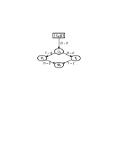
Figure 2: Classification of spaces satisfying the metricity condition

Spin connection. Linear connection and metric are geometric objects independent of the choice of frame. Their components are defined with respect to a frame and are, clearly, frame-dependent. The choice of frame in $T_{P}$ is not unique; $C$ frames $\hbox{\boldmath$e$}_{\mu}$ and $L$ frames $\hbox{\boldmath$e$}_{i}$ are of particular practical importance. Every tangent vector $u$ can be expressed in both frames: $\hbox{\boldmath$u$}=u^{\mu}\hbox{\boldmath$e$}_{\mu}=u^{i}\hbox{\boldmath$e$}_{i}$. In particular, $\hbox{\boldmath$e$}_{i}=e_{i}{{}^{\mu}}\hbox{\boldmath$e$}_{\mu}$, $\hbox{\boldmath$e$}_{\mu}=e^{i}{{}_{\mu}}\hbox{\boldmath$e$}_{i}$, and accordingly, $u^{i}=e^{i}{{}_{\mu}}u^{\mu}$, $u^{\mu}=e_{i}{{}^{\mu}}u^{i}$. The scalar product of two tangent vectors can be written in two equivalent forms: $\hbox{\boldmath$u$}\cdot\hbox{\boldmath$v$}=g_{\mu\nu}u^{\mu}v^{\nu}=\eta_{ij}u^{i}v^{j}$, where

$$\eta_{ij}=\hbox{\boldmath$e$}_{i}\cdot\hbox{\boldmath$e$}_{j}=g_{\mu\nu}e_{i}{{}^{\mu}}e_{j}{{}^{\nu}}\,,\qquad g_{\mu\nu}=\hbox{\boldmath$e$}_{\mu}\cdot\hbox{\boldmath$e$}_{\nu}=\eta_{ij}e^{i}{{}_{\mu}}e^{j}{{}_{\nu}}\,.$$

The parallel transport of a tangent vector $\hbox{\boldmath$u$}\in T_{x}$, represented in the form $\hbox{\boldmath$u$}=u^{i}\hbox{\boldmath$e$}_{i}$, is defined by the parallel transport rule

$$\delta u^{i}=-\omega^{i}{}_{j\mu}u^{j}dx^{\mu}\,,$$

where $\omega^{ij}{{}_{\mu}}$ is the so-called spin connection, with 64 components. Parallel transport of $v_{i}$ is determined by requiring $\delta(u^{i}v_{i})=0$: $\delta v_{i}=\omega^{j}{}_{i\mu}v_{j}dx^{\mu}$. An equivalent definition of the parallel transport may be given in terms of the $\omega$-covariant derivative:

$$D(\omega)u^{i}=\bigl{(}\partial_{\mu}u^{i}+\omega^{i}{}_{j\mu}u^{j}\bigr{)}dx^{\mu}\equiv D_{\mu}(\omega)u^{i}dx^{\mu}\,,$$ (2.7)

and similarly for $v_{i}$.

The existence of $L$ frames at each point of $X_{4}$ implies the existence of the Lorentz metric $\eta_{ij}$ at each point of $X_{4}$. Demanding the tensor field $\eta_{ij}$ to be invariant under the parallel transport, implies that the connection is antisymmetric in its Latin indices:

$$\delta\eta_{ij}=\bigl{(}\omega^{s}{}_{i\mu}\eta_{sj}+\omega^{s}{}_{j\mu}\eta_{si}\bigr{)}dx^{\mu}=\bigl{(}\omega_{ji\mu}+\omega_{ij\mu}\bigr{)}dx^{\mu}=0\,.$$

Since $\eta$ is a constant tensor, its covariant derivative vanishes:

$$D_{\mu}(\omega)\eta_{ij}=0\,.$$ (2.8)

Relation between $\omega$ and $\Gamma$. The parallel transport is a unique geometric operation, independent of the choice of frame, hence

$$u^{i}+\delta u^{i}=(u^{\mu}+\delta u^{\mu})e^{i}{{}_{\mu}}(x+dx)\,.$$

From this property, we obtain the relation between $\omega$ and $\Gamma\,$, called the tetrad postulate:

$$D_{\mu}(\omega+\Gamma)e^{i}{{}_{\nu}}\equiv D_{\mu}(\omega)e^{i}{{}_{\nu}}-\Gamma^{\rho}_{\nu\mu}e^{i}{{}_{\rho}}=0\,,$$ (2.9)

where $D_{\mu}(\omega)e^{i}{{}_{\mu}}=\partial_{\mu}e^{i}{{}_{\nu}}+\omega^{i}{}_{j\mu}e^{j}{{}_{\nu}}$. The operator $D(\omega+\Gamma)$ can be formally understood as a “total” covariant derivative. Using the above equations we easily derive the metricity condition:

$$D_{\mu}(\Gamma)g_{\mu\nu}=D_{\mu}(\omega+\Gamma)g_{\mu\nu}=D_{\mu}(\omega+\Gamma)(\eta_{ij}e^{i}{{}_{\mu}}e^{j}{{}_{\nu}})=0\,.$$

The $\omega$-covariant derivative can be generalized to a quantity $\phi$ belonging to an arbitrary representation of the Lorentz group:

$$D_{\mu}(\omega)\phi=\bigl{(}\partial_{\mu}+\omega_{\mu}\bigr{)}\phi\,,\qquad\omega_{\mu}\equiv\hbox{${1\over 2}$}\omega^{ij}{{}_{\mu}}\Sigma_{ij}\,,$$ (2.10)

where $\Sigma$ is the related spin matrix.

It is interesting to note that if we find $\Gamma=\Gamma(\omega)$ from equation (2.9) and substitute the result into the expressions (2.3) and (2.4) for the torsion and the curvature, we obtain

(2.11)

Equation (LABEL:eq:2.11a) can be formally solved for the connection $\omega$:

where $c^{i}{}_{\mu\nu}=\partial_{\mu}e^{i}{{}_{\nu}}-\partial_{\nu}e^{i}{{}_{\mu}}$ is called the object of anholonomity, and $K$ is the contortion.

Geometric interpretation of PGT

The final result of the analysis of PGT is the construction of the invariant Lagrangian (1). It is achieved by introducing new fields $A^{ij}{{}_{\mu}}$ and $b^{i}{{}_{\mu}}$ (or $h_{k}{{}^{\nu}}$), which are used to construct the covariant derivative $\nabla_{k}=h_{k}{{}^{\nu}}\nabla_{\nu}$ and the field strengths $F^{ij}{{}_{\mu\nu}}$ and $F^{i}{{}_{\mu\nu}}$. This theory can be thought of as a field theory in Minkowski space. However, geometric analogies are so strong, that it would be unnatural to ignore them.

Table 1. Relation between PGT (left) and Riemann–Cartan geometry
$A^{ij}{{}_{\mu}}$ Lorentz gauge field	$\omega^{ij}{{}_{\mu}}$ spin connection
$\nabla_{\mu}(A)$ covariant derivative	$D_{\mu}(\omega)$ $\omega$-covariant derivative
$b^{i}{{}_{\mu}}~{}~{}(h_{k}{{}^{\nu}})$ transl. gauge field	$e^{i}{{}_{\mu}}~{}~{}(e_{k}{{}^{\nu}})$ tetrad coframe (frame)
$\Gamma^{\rho}_{\mu\nu}$ not defined	$\Gamma^{\rho}_{\mu\nu}$ connection
tetrad postulate! $\Rightarrow$ $\Gamma^{\rho}_{\mu\nu}$ defined	$D_{\mu}(\omega)e^{i}{{}_{\nu}}=\Gamma^{\rho}_{\nu\mu}e^{i}{{}_{\rho}}$ tetrad postulate
$\nabla_{\mu}\eta_{ij}=0$ metricity condition	$D_{\mu}(\Gamma)g_{\nu\l}=0$ metricity condition
$F^{i}{}_{\mu\nu}=\nabla_{\mu}b^{i}{{}_{\nu}}-\nabla_{\nu}b^{i}{{}_{\mu}}$	$T^{i}{}_{\mu\nu}=(\Gamma^{\rho}_{\nu\mu}-\Gamma^{\rho}_{\mu\nu})b^{i}{{}_{\rho}}=T^{i}{}_{\mu\nu}(\omega)$
$F^{ij}{}_{\mu\nu}=F^{ij}{}_{\mu\nu}(A)$	$R^{ij}{}_{\mu\nu}=R^{ij}{}_{\mu\nu}(\omega)$

$\alpha)$ The Lorentz gauge field $A^{ij}{{}_{\mu}}$ can be identified with the spin connection $\omega^{ij}{{}_{\mu}}$, as follows from its transformation law (LABEL:eq:1.9a). Equivalently, $\nabla_{\mu}(A)$ can be identified with the geometric covariant derivative $D_{\mu}(\omega)$. This follows from the definition of $\nabla_{\mu}\phi$, which implies that a) the quantity $\nabla_{\mu}\phi$ has one additional dual index, as compared to $\phi$; b) it acts linearly, obeys Leibniz rule, commutes with contraction, and $\nabla_{\mu}f=\partial_{\mu}f$ if $f$ is a scalar function.

$\beta)$ The field $b^{i}{{}_{\mu}}$ can be identified with $e^{i}{{}_{\mu}}$, on the basis of its transformation law (LABEL:eq:1.9b). It ensures the possibility to transform local Lorentz and coordinate indices into each other.

$\gamma)$ Local Lorentz symmetry of PGT implies the metricity condition (2.8). After adopting the tetrad postulate (2.9), whereby one introduces the connection $\Gamma^{\rho}_{\nu\mu}$ in PGT, the metricity condition (2.8) becomes equivalent to (2.5).

$\delta)$ It follows from equations (2.11) that the translation field strength $F^{i}{{}_{\mu\nu}}$ is nothing but the torsion $T^{i}{}_{\mu\nu}$, while the Lorentz field strength $F^{ij}{}_{\mu\nu}$ represents the curvature $R^{ij}{}_{\mu\nu}$.

• Consequently, PGT has the geometric structure of Riemann–Cartan space $U_{4}$.

Although PGT has a well defined geometric interpretation, its gauge structure differs from what we have in “standard” gauge theories (Appendix A).

The principle of equivalence in PGT

The principle of equivalence (PE) is a dynamical principle, which severely restricts the form of the gravitational interaction. It states that $i)$ the effect of gravity on matter is locally equivalent to the effect of a non-inertial reference frame in special relativity (SR).

To clarify the dynamical content of the PE, let us consider an inertial frame in $M_{4}$, in which (massive) matter field $\phi$ is described by a Lagrangian ${\cal L}_{M}(\phi,\partial_{i}\phi)$. When we go over to a non-inertial frame, ${\cal L}_{M}$ transforms into $b{\cal L}_{M}(\phi,\nabla_{i}\phi)$, with $\nabla_{i}=e_{i}{{}^{\mu}}(\partial_{\mu}+\omega_{\mu})$. The pseudo-gravitational field, equivalent to the non-inertial reference frame, is contained in $b$ and $\nabla_{i}$. This field can be eliminated on the whole spacetime by simply going back to the global inertial frame, while for real gravitational fields this is not true — they can be eliminated only locally, as we shall see. For this reason, in the last step of introducing a real gravitational field, Einstein replaced $M_{4}$ with a Riemann space $V_{4}$. Although this is a correct choice, we shall see that Einstein could have chosen also a Riemann–Cartan space $U_{4}$.

Let us now recall another formulation of the PE:  $ii)$ the effect of gravity on matter can be locally eliminated by a suitable choice of reference frame, whereupon matter behaves as in SR. More precisely,

• at any point $P$ in spacetime one can choose an orthonormal reference frame $\hbox{\boldmath$e$}_{i}$, such that: a) $\omega^{ij}{{}_{\mu}}=0$,  b) $e_{i}{{}^{\mu}}=\delta_{i}^{\mu}$,  at $P$.

We shall see that this statement is correct not only in GR ($V_{4}$), but also in PGT ($U_{4}$) [12, 13].

Gravitational theory in Riemann space $V_{4}$ possesses certain features which do not follow necessarily from the PE. Namely, the form of Riemannian connection shows that relative orientation of the orthonormal frame $\hbox{\boldmath$e$}_{i}(x+dx)$ with respect to $\hbox{\boldmath$e$}_{i}(x)$ (parallel transported to $x+dx$) is completely fixed by the metric. The change of this orientation is described by Lorentz transformations, which do not produce any gravitational effect; therefore, there is no reason to prevent any additional Lorentz rotation of local frames. If we want to realize this freedom, the spin connection should contain an extra part, independent of the metric: $\omega^{i}{}_{j\mu}\equiv\Delta^{i}{}_{j\mu}+K^{i}{}_{j\mu}$. Interpreted in this way, the PE becomes nicely incorporated into Riemann–Cartan geometry, as shown bellow.

Let $\hbox{\boldmath$e$}_{i}$ be a basis for $T_{P}$ in spacetime. For each $i$, one can define an auto-parallel $C_{i}$ through $P$, with tangent vector $\hbox{\boldmath$e$}_{i}$. By parallel transporting $\hbox{\boldmath$e$}_{i}$, one can define a vector field $\hbox{\boldmath$e$}_{i}$ along $C_{i}$, in some neighborhood ${\cal O}_{i}$. Taking a suitable restriction of the intersection of all ${\cal O}_{i}$, we can find a neighborhood ${\cal O}$ of $P$ in which the auto-parallels $C_{i}$ do not intersect. The set of vector fields $\hbox{\boldmath$e$}_{i}$ can be extended to form a parallel frame on ${\cal O}$. Hence, the connection coefficients at $P$, defined with respect to this particular frame, vanish: $\Gamma^{i}_{jk}(P)=0$. This result makes no use of any metric property, and holds for an arbitrary linearly connected manifold [13]. In $U_{4}$, the parallel frame on ${\cal O}$ can be made orthonormal, $\hbox{\boldmath$e$}_{i}\cdot\hbox{\boldmath$e$}_{j}=\eta_{ij}$, which gives an attractive physical content to the PE. Using the formula $\Gamma^{i}_{jk}=e_{k}{{}^{\rho}}\omega^{i}{}_{j\rho}$, we conclude that $\omega^{ij}{{}_{\mu}}(P)=0$.

At each point $P$ in ${\cal O}$, one can introduce local inertial coordinates, defined by $dx^{i}=e^{i}{{}_{\mu}}dx^{\mu}$. Let us now change the coordinates $x^{\mu}$, $x^{\mu}\to y^{\mu}$, so that $y^{\mu}$ coincide with $x^{i}$ at $P$: $dy^{\mu}=\delta^{\mu}_{i}dx^{i}$. This coordinate transformation ensures $e_{i}{{}^{\mu}}(P)=\delta_{i}^{\mu}$, without changing $\omega^{ij}{{}_{\mu}}(P)=0$.

• The existence of torsion does not violate the PE.

The PE fits naturally into a $U_{4}$ geometry of spacetime. In particular, it holds in $V_{4}$, and also in $T_{4}$. In more general geometries, where the symmetry of the tangent space is higher than the Poincaré group, the usual form of the PE is violated, and local physics is different from SR [9, 8].

3 The teleparallel theory

Dynamics of the gravitational field in PGT is determined by the form of the gravitational Lagrangian ${\cal L}_{G}$. If we demand that the equations of motion are at most of second order in field derivatives, ${\cal L}_{G}$ can be at most quadratic in torsion and curvature. A lot of different invariants makes the general structure of ${\cal L}_{G}$ rather complicated: ${\cal L}_{G}\sim R+T^{2}+R^{2}+\l$, with eleven $(1+3+6+1)$ constant parameters [7].

The simple action

$$I_{\rm EC}=\int d^{4}xb(-aR+{\cal L}_{M})\,,\qquad a=\frac{1}{16\pi G}\,,$$

defines the so-called Einstein–Cartan (EC) theory, a direct generalization of GR to Riemann–Cartan spacetime [3, 4]. The EC theory incorporates both mass and spin of matter as sources of the gravitational field, and represent a description of gravity which is microscopically more satisfying than GR. Indeed, in current theories of fundamental interactions matter is described by matter fields, with their spins, symmetries and conserved currents; at this level, there is no space for the conventional GR, with matter consisting of point particles, fluids and light rays. On the other hand, spin effects are negligible for macroscopic matter, so that the empirical predictions of the EC theory are, for all practical purposes, the same as in GR. A simple but accurate way to depict this situation is to name GR “the best available alternative gravitational theory”, the best theory being the EC theory itself [14]. Since the structure of the EC theory is pretty well known, we turn our attention to the teleparallel theory as “the next best” alternative [14].

General geometric arena of PGT, the Riemann–Cartan space $U_{4}$, may be a priori restricted by imposing certain conditions on the curvature and the torsion. Thus, Einstein’s GR is defined in Riemann space $V_{4}$, obtained from $U_{4}$ by the requirement of vanishing torsion. Another interesting limit of PGT is Weitzenböck or teleparallel geometry $T_{4}$, defined by the requirement

$$R^{ij}{}_{\mu\nu}(A)=0\,.$$ (3.1)

The vanishing of curvature means that parallel transport is path independent (if some topological restrictions are adopted), hence we have an absolute parallelism. The teleparallel geometry is, in a sense, complementary to Riemannian: curvature vanishes, and torsion remains to characterize the parallel transport.

The physical interpretation of the teleparallel geometry is based on the fact that there is a one-parameter family of teleparallel Lagrangians which is empirically equivalent to GR [15, 16, 17].

Lagrangian. In the framework of the teleparallel geometry $T_{4}$, gravitational field is described by the tetrad $b^{k}{{}_{\mu}}$ and Lorentz connection $A^{ij}{{}_{\mu}}$, subject to the condition of vanishing curvature. We shall consider here the gravitational dynamics determined by a class of Lagrangians quadratic in the torsion:

where $\l_{ij}{}^{\mu\nu}$ are Lagrange multipliers introduced to ensure the teleparallelism condition (3.1) in the variational formalism, and $\beta_{ijk}=a\bigl{(}AT_{ijk}+BT_{[jik]}+C\eta_{i[j}T_{k]}\bigr{)}$.

The parameters $A,B,C$ in the Lagrangian should be determined on physical grounds, so as to obtain a consistent theory which could describe all the known gravitational experiments. If we require that the theory (LABEL:eq:3.2) gives the same results as GR in the linear, weak-field approximation, we can restrict our considerations to the one-parameter family of Lagrangians, defined by the conditions [15, 16, 17]

$i)$ $\,2A+B+C=0\,,\quad C=-1$.

This family represents a viable gravitational theory for macroscopic matter (scalar and electromagnetic fields), empirically indistinguishable from GR. Von der Heyde and Hehl have given certain theoretical arguments in favor of the choice $B=0$ [6]. There is, however, another, particularly interesting choice determined by the requirement

$ii)$ $\,2A-B=0$.

In the gravitational sector, this choice leads effectively to the Einstein–Hilbert Lagrangian of GR, ${\cal L}_{EH}=-abR(\Delta)$, with Riemannian connection $A=\Delta$. To see that, we substitute the expression (1) for the spin connection, $A=\Delta+K$, into the definition of the scalar curvature tensor $R(A)$, and obtain the geometric identity

$$abR(A)=abR(\Delta)+{\cal L}_{T}^{\parallel}-2a\partial_{\rho}(bT^{\rho})\,,$$ (3.3)

where ${\cal L}_{T}^{\parallel}$ is the torsion Lagrangian (LABEL:eq:3.2) with

$$A=\hbox{${1\over 4}$}\,,\qquad B=\hbox{${1\over 2}$}\,,\qquad C=-1\,.$$ (3.4)

The conditions $i)$ and $ii)$ given above coincide with (3.4). In the teleparallel spacetime, where $R(A)=0$, the identity (3.3) implies the relation ${\cal L}_{T}^{\parallel}={\cal L}_{EH}$ + divergence; that is why the teleparallel theory (LABEL:eq:3.2) with ${\cal L}_{T}={\cal L}_{T}^{\parallel}$ is called the teleparallel formulation of GR (GR_∥). It is equivalent to GR for scalar and electromagnetic matter (see Lecture 1), but the other matter fields have different couplings in $T_{4}$ and $V_{4}$.

Field equations. By varying the Lagrangian (LABEL:eq:3.2) with respect to $b^{i}{{}_{\mu}},A^{ij}{{}_{\mu}}$ and $\l_{ij}{}^{\mu\nu}$, we obtain the gravitational field equations [18]:

(3.5)

The third field equation defines the teleparallel geometry in PGT. The first field equation is a dynamical equation for $b^{k}{{}_{\mu}}$. The symmetric part of this equation plays the role analogous to Einstein’s equation in GR, while the antisymmetric part implies

$$4\nabla_{\mu}(b\beta_{[ij]}{{}^{\mu}})\approx\tau_{[ji]}\,.$$ (3.6a)

In GR_∥, the left hand side vanishes, so that $$\tau_{[ij]}$$ must also vanish. Since this is not true for Dirac field, it follows that the description of Dirac matter in GR_∥ is not consistent. In the one-parameter teleparallel theory the left hand side is proportional to the axial torsion, and we do not have any problem. By taking the covariant divergence of (LABEL:eq:3.5b), one obtains the consistency condition

$$-8\nabla_{\mu}\bigl{(}b\beta_{[ij]}{{}^{\mu}}\bigr{)}\approx\nabla_{\mu}\sigma^{\mu}{}_{ij}\,.$$ (3.6b)

This condition is satisfied as a consequence of (3.6a) and the second identity in (LABEL:eq:1.14). Thus, the only role of (LABEL:eq:3.5b) is to determine the Lagrange multipliers $\l_{ij}{}^{\mu\nu}$. Taking into account equation (3.6b), one concludes that the number of independent equations (LABEL:eq:3.5b) is $24-6=18$. It is clear that these equations cannot determine 36 multipliers $\l_{ij}{}^{\mu\nu}$ in a unique way. As we shall see, non-uniqueness of $\l_{ij}{}^{\mu\nu}$ is related to an extra gauge freedom in the theory.

The $\lambda$ symmetry. The gravitational Lagrangian (LABEL:eq:3.2) is, by construction, invariant under the local Poincaré transformations. In addition, it is also invariant, up to a four-divergence, under the transformations [18]

$$\delta_{0}\l_{ij}{}^{\mu\nu}=\nabla_{\rho}\varepsilon_{ij}{}^{\mu\nu\rho}\,,$$ (3.7a)

where the gauge parameter $$\varepsilon_{ij}{}^{\mu\nu\rho}=-\varepsilon_{ji}{}^{\mu\nu\rho} 6\times 4=24 \varepsilon^{\l\rho\mu\nu}\nabla_{\rho}R^{ij}{}_{\mu\nu}=0 R^{ij}{}_{\mu\nu}=0 \l$$ is completely antisymmetric in its upper indices, and has components. The invariance is easily verified by using the second Bianchi identity . On the other hand, the invariance of the field equation (LABEL:eq:3.5b) follows directly from . The symmetry (3.7a) will be referred to as symmetry.

It is useful to observe that the $\l$ transformations can be written in the form

$$\delta_{0}\l_{ij}{}^{\alpha\beta}=\nabla_{0}\varepsilon_{ij}{}^{\alpha\beta}+\nabla_{\gamma}\varepsilon_{ij}{}^{\alpha\beta\gamma}\,,\qquad\delta_{0}\l_{ij}{}^{0\beta}=\nabla_{\gamma}\varepsilon_{ij}{}^{\beta\gamma}\,,$$ (3.7b)

where $\varepsilon_{ij}{}^{\alpha\beta}\equiv\varepsilon_{ij}{}^{\alpha\beta 0}$. However, one can show by canonical methods (Appendix B) that

• the only independent parameters of the $\l$ symmetry are $\varepsilon_{ij}{}^{\alpha\beta}$.

The six parameters $\varepsilon_{ij}{}^{\alpha\beta\gamma}$ are not independent of $\varepsilon_{ij}{}^{\alpha\beta}$. Hence, they can be completely discarded, leaving us with $24-6=18$ independent gauge parameters. They can be used to fix 18 multipliers $\l_{ij}{}^{\mu\nu}$, whereupon the remaining 18 multipliers are determined by the independent field equations (LABEL:eq:3.5b) (at least locally).

The Poincaré and $\l$ gauge symmetries are always present (sure symmetries), independently of the values of parameters $A,B$ and $C$ in the teleparallel theory (LABEL:eq:3.2). Specific models, such as GR_∥, may have extra gauge symmetries, which are present only for some critical values of the parameters. The gauge structure of the one-parameter teleparallel theory is problematic [19].

OT frames. Teleparallel theories in $U_{4}$ are based on the condition of vanishing curvature. Let us choose an arbitrary tetrad at point $P$ of spacetime. Then, by parallel transporting this tetrad to all other points, we generate the tetrad field on spacetime manifold. If the manifold is paralellizable (which is a strong topological assumption), the vanishing of curvature implies that the parallel transport is path independent, so the resulting tetrad field is globally well defined. In such an orthonormal and teleparallel (OT) frame, the connection coefficients vanish:

$$A^{ij}{{}_{\mu}}=0\,.$$ (3.8)

The above construction is not unique — it defines a class of OT frames, related to each other by global Lorentz transformations. In an OT frame, the covariant derivative reduces to the partial derivative, and the torsion takes the simple form: $T^{i}{}_{\mu\nu}=\partial_{\mu}b^{i}{{}_{\nu}}-\partial_{\nu}b^{i}{{}_{\mu}}$ (see e.g. [20]).

Equation (3.8) defines a particular solution of the condition $R^{ij}{}_{\mu\nu}(A)=0$. Since a local Lorentz transformation of the tetrad field induces a non-homogeneous change in the connection,

$$e^{\prime}{{}^{i}}{{}_{\mu}}=\L^{i}{{}_{k}}e^{k}{{}_{\mu}}\quad\Rightarrow\quad A^{\prime ij}{{}_{\mu}}=\L^{i}{{}_{m}}\L^{j}{{}_{n}}A^{mn}{{}_{\mu}}+\L^{i}{{}_{m}}\partial_{\mu}\L^{jm}\,,$$

it follows that the general solution of $R^{ij}{}_{\mu\nu}(A)=0$ has the form $A^{ij}{{}_{\mu}}=\L^{i}{{}_{m}}\partial_{\mu}\L^{jm}$. Thus, the choice (3.8) breaks local Lorentz invariance, and represents a gauge fixing condition.

In the action (LABEL:eq:3.2), the condition of teleparallelism is ensured by the Lagrange multiplier. The field equation (LABEL:eq:3.5b) merely serves to determine the multiplier, while the non-trivial dynamics is completely contained in (LABEL:eq:3.5a). Hence, the teleparallel theory (on parallelizable manifolds) may also be described by imposing the gauge condition (3.8) directly in the action. The resulting theory is defined in terms of the tetrad field only, and may be thought of as the gauge theory of translations. This formalism is often used in the literature because of its technical simplicity, but the local Lorentz-invariant formulation simplifies the canonical analysis of the conservation laws.

Exact solutions. It is interesting to see how some exact solutions of the one-parameter theory can be obtained by a simple analysis of the field equations [21, 22]. We start with the torsion Lagrangian of the one-parameter theory, written in the form

$${\cal L}_{T}={\cal L}_{T}^{\parallel}-\frac{a}{12}(2B-1){\cal A}_{ijk}{\cal A}{}^{ijk}\,,\qquad{\cal A}_{ijk}\equiv T_{ijk}+T_{kij}+T_{jki}\,,$$ (3.9)

where ${\cal L}_{T}^{\parallel}$ is the torsion Lagrangian of GR_∥. Using the geometric identity (3.3), it follows that the first field equation has the form

$$R_{ik}(\Delta)-\hbox{${1\over 2}$}\eta_{ik}R(\Delta)+{\cal O}({\cal A})=\tau_{ki}/2ab\,,$$ (3.10)

where ${\cal O}({\cal A})$ are terms proportional to ${\cal A}_{ijk}$. For $2B-1=0$ the above Lagrangian reduces to the GR form, and equations (3.10) coincides with Einstein’s equations. More generally, for any field configurations satisfying ${\cal A}_{ijk}=0$, the first field equation has the same form as in GR. The consistency of this equation requires $\tau_{ki}$ to be symmetric.

Taking into account that the second field equation serves only to determine the Lagrange multipliers $\l_{ij}{}^{\mu\nu}$, we can use this result to generate some solutions of the teleparallel theory, starting from certain solutions of GR. Consider, for instance, a metric which has diagonal form in some coordinate system:

$$ds^{2}=A(dx^{0})^{2}-B_{1}(dx^{1})^{2}-B_{2}(dx^{2})^{2}-B_{3}(dx^{3})^{2}\,.$$ (3.11a)

Let us choose the tetrad components to be diagonal,

$$b^{0}{}_{0}=\sqrt{A}\,,\qquad b^{a}{{}_{\alpha}}=\delta^{a}_{\alpha}\sqrt{B_{\alpha}}\,,$$ (3.11b)

and fix the gauge $A^{ij}{}_{\mu}=0$. Then, one easily proves that ${\cal A}_{ijk}=0$, and derives an important consequence:

• If the diagonal metric (3.11a) is a solution of GR, the related tetrad (3.11b) is a solution of the one-parameter theory, in the gauge $A^{ij}{{}_{\mu}}=0$ and with the same $\tau_{ik}$.

An important class of solutions of this type is the class of spherically symmetric solutions.

All observational differences from GR are related to the effects stemming from ${\cal A}_{ijk}\neq 0$.

On the physical interpretation. We have seen that the field equations of GR_∥ are identical to those of GR for macroscopic matter (scalar and electromagnetic fields), but the coupling of Dirac field is not consistent. What happens in the one-parameter theory? The related argument about Dirac matter coupling does not hold any more: the antisymmetric part of the first field equation (3.10) shows that $\tau_{[ij]}$ is proportional to the axial torsion ${\cal A}_{klm}$ contained in ${\cal O}({\cal A})$. Thus, it seems that one should abandon GR_∥ and use the one-parameter theory in order to consistently describe Dirac matter. However, serious arguments given in Refs. [19] strongly indicate that the gauge structure of the one-parameter theory (the initial value problem and the canonical formulation) is problematic. Unless the problem is solved in a satisfactory way, one should remain skeptical about the idea of treating this theory as a fundamental approach to gravity.

The situation just described led some authors to interpret the teleparallel theory only as an effective macroscopic theory of gravity [16]. If we accept this point of view, we can investigate experimental predictions of the theory by using test particles/fields of any type (scalars, spinors, etc). Possible empirical differences between GR and the one-parameter teleparallel theory can be tested by measuring non-trivial axial torsion effects [21, 23].

Concluding remarks

We conclude the exposition with a short summary.

1) PGT is based on the global Poincaré symmetry, a well established symmetry in particle physics, and incorporates both mass and spin as sources of the gravitational field.

2) The geometric interpretation of PGT leads to Riemann–Cartan geometry of spacetime, in which both curvature and torsion are used to characterize the gravitational phenomena. Riemann–Cartan geometry is compatible with the principle of equivalence.

3) The EC version of PGT is microscopically more satisfying then GR, while its macroscopic predictions are, for all practical purposes, the same as in GR.

4) In the teleparallel limit of PGT, curvature vanishes and torsion remains to characterize both the geometry of spacetime and the gravitational dynamics. The general one-parameter theory, including GR_∥ as a special case, is empirically equivalent to GR. In spite of that, the existing consistency problems make it difficult to accept the teleparallel theory as a fundamental theory of gravity.

Acknowledgements

I would like to thank M. Vasilić, F. W. Hehl and J. Garecki for useful discussions.

Appendix A: On the gauge structure of PGT

It is an intriguing fact that PGT does not have the structure of an “ordinary” gauge theory [24]. To clarify this point, we start from the Poincaré generators $P_{a},M_{ab}$ and define the gauge potential as $A_{\mu}=e^{a}{{}_{\mu}}P_{a}+\hbox{${1\over 2}$}\omega^{ab}{{}_{\mu}}M_{ab}$. The infinitesimal gauge transformation

$$\delta_{0}A_{\mu}=-\tilde{\nabla}_{\mu}\l\equiv-\partial_{\mu}\l-[A_{\mu},\l]\,,$$

where $\l=\l^{a}P_{a}+\hbox{${1\over 2}$}\l^{ab}M_{ab}$, has the following component content:

where $\nabla=\nabla(\omega)$ is the covariant derivative with respect to the spin connection $\omega$. The resulting gauge transformations are clearly different from those obtained in PGT.

Although the tetrad field and the spin connection carry a representation of the Poincaré group, the EC action in four dimensions, $I_{EC}=\hbox{${1\over 4}$}\int d^{4}x\varepsilon^{\mu\nu\l\rho}\varepsilon_{abcd}e^{c}{{}_{\l}}e^{d}{{}_{\rho}}R^{ab}{}_{\mu\nu}$, is not invariant under the translational part of the Poincaré group,

$$\delta_{T}I_{EC}=\hbox{${1\over 4}$}\int d^{4}x\varepsilon^{\mu\nu\l\rho}\varepsilon_{abcd}\l^{c}T^{d}{}_{\l\rho}R^{ab}{}_{\mu\nu}\neq 0\,,$$

but it remains invariant under Lorentz rotations and diffeomorphisms. The situation is different in 3d, where gravity can be represented as a “true” gauge theory [25].

Appendix B: Canonical generator of the $\l$ symmetry

The canonical analysis of a gauge theory is the best way to explain its gauge structure. We apply this approach to examine the $\l$ symmetry in the teleparallel theory [18].

The basic phase space dynamical variables of the teleparallel theory (LABEL:eq:3.2) are $(b^{i}{}_{\mu},A^{ij}{}_{\mu},\l_{ij}{}^{\mu\nu})$ and the corresponding momenta $(\pi_{i}{}^{\mu},\pi_{ij}{}^{\mu},\pi^{ij}{}_{\mu\nu})$. Going through the standard Dirac type analysis, one can find all the constraints and the total Hamiltonian. Then, starting from the primary first class constraint $\pi^{ij}{}_{\alpha\beta}$, one can apply the general canonical procedure and show that the canonical gauge generator acting on the Lagrange multipliers $\l_{ij}{}^{\mu\nu}$ has the form

Using the rule $$\delta_{0}X=\int d^{3}x^{\prime}\{X,G^{\prime}\} \l$$, we apply the generator (LABEL:eq:B.1a) to the field, and find

$$\delta_{0}^{A}\l_{ij}{}^{0\alpha}=\nabla_{\beta}\,\varepsilon_{ij}{}^{\alpha\beta}\,,\qquad\delta_{0}^{A}\l_{ij}{}^{\alpha\beta}=\nabla_{0}\,\varepsilon_{ij}{}^{\alpha\beta}\,,$$ (B.1b)

as the only non-trivial transformations. Surprisingly, this result does not agree with the form of the $\l$ symmetry (3.7b), which contains an additional piece, $\nabla_{\gamma}\varepsilon_{ij}{}^{\alpha\beta\gamma}$, in the expression for $\delta_{0}\l_{ij}{}^{\alpha\beta}$. Since there are no other primary first class constraints that could produce the transformation of $\l_{ij}{}^{\alpha\beta}$, the canonical origin of the additional term seems somewhat puzzling.

The solution of the problem is, however, quite simple: if we consider only independent gauge transformations, this term is not needed. To prove this statement, consider the following primary first class constraint

$$\Pi^{ij}{}_{\alpha\beta\gamma}=\nabla_{\alpha}\pi^{ij}{}_{\beta\gamma}+\nabla_{\gamma}\pi^{ij}{}_{\alpha\beta}+\nabla_{\beta}\pi^{ij}{}_{\gamma\alpha}\,,$$

which is essentially a linear combination of $\pi^{ij}{}_{\alpha\beta}$. Hence, the related gauge generator will not be truly independent of the general expression (LABEL:eq:B.1a). The standard canonical construction yields

$$G_{B}[\varepsilon]=-\frac{1}{4}\int d^{3}x\,\varepsilon_{ij}{}^{\alpha\beta\gamma}\nabla_{\alpha}\pi^{ij}{}_{\beta\gamma}\,,$$ (B.2a)

where the parameter $$\varepsilon_{ij}{}^{\alpha\beta\gamma}$$ is totally antisymmetric with respect to its upper indices. The only non-trivial field transformation produced by this generator is

$$\delta_{0}^{B}\l_{ij}{}^{\alpha\beta}=\nabla_{\gamma}\varepsilon_{ij}{}^{\alpha\beta\gamma}\,,$$ (B.2b)

and it coincides with the missing term in equation (B.1b). Thus, if we are interested only in the independent $\l$ transformations,

• the six parameters $\varepsilon_{ij}{}^{\alpha\beta\gamma}$ in the $\l$ transformations (3.7b) can be completely discarded.

Although the generator $G_{B}$ is not truly independent of $G_{A}$, it is convenient to define $G\equiv G_{A}+G_{B}$ as an overcomplete gauge generator, since it automatically generates the covariant Lagrangian form of the $\l$ symmetry.

References

- [1]
- [2] [] The list of references is prepared so as to properly represent the ideas presented in the lectures, without an intention of being complete.
- [3] T. W. B. Kibble, Lorentz invariance and the gravitational field, J. Math. Phys. 2 (1961) 212; see also R. Utiyama, Invariant theoretical interpretation of interactions, Phys. Rev. 101 (1956) 1597.
- [4] D. W. Sciama, On the analogy between charge and spin in general relativity, in: Recent Developments in General Relativity, Festschrift for Infeld (Pergamon Press, Oxford, 1962), p. 415.
- [5] F. W. Hehl, P. von der Heyde. D. Kerlick and J. Nester, General relativity with spin and torsion: Foundations and prospects, Rev. Mod. Phys. 48 (1976) 393.
- [6] F. W. Hehl, Four lectures in Poincaré gauge theory, in Cosmology and Gravitation: Spin, Torsion, Rotation and Supergravity, eds. P. G. Bergmann and V. de Sabbata (Plenum, New York, 1980) p. 5.
- [7] K. Hayashi and T. Shirafuji, Gravity from the Poincaré gauge theory of fundamental interactions, Prog. Theor. Phys. 64 (1980) 866, 883, 1435, 2222.
- [8] M. Blagojević, Gravitation and gauge symmetries (IoP Publishing, Bristol, 2002).
- [9] F. W. Hehl, J. D. McCrea, E. W. Mielke and Y. Ne’eman, Metric-affine gauge theory of gravity: field equations, Noether identities, world spinors and breaking of dilation invariance, Phys. Rep. C258 (1995) 1.
- [10] F. W. Hehl, Spin and torsion in general relativity, Gen. Rel. Grav. 4 (1973) 333, 5 (1974) 491; L. Smalley, On the extension of geometric optics from Riemannian to Riemann–Cartan spacetime, Phys. Lett. 117A (1986) 267.
- [11] Y. Choquet–Bruhat, C. De Witt–Morette and M. Dillard–Bleik, Analysis, manifolds and physics (North Holland, Amsterdam, 1977). B. Dubrovin, S. Novikov and A. Fomenko, Sovremennaya Geometriya (Nauka, Moskow, 1979), in Russian.
- [12] P. von der Heyde, The equivalence principle in the theory of gravitation, Nuovo Cim. Lett. 14 (1975) 250.
- [13] D. Hartley, Normal frames for non-Riemannian connections, Class. Quant. Grav. 12 (1995) L103.
- [14] F. W. Hehl, Alternative Gravitational Theories in Four Dimensions, Report of parallel session chair in: Proc. 8th M. Grossmann Meeting, T. Pirani (ed.) (World Scientific, Singapore, 1998), preprint gr-qc/9712096.
- [15] K. Hayashi and T. Shirafuji, New general relativity, Phys. Rev. D19 (1979) 3524.
- [16] F. W. Hehl, J. Nitsch and P. von der Heyde, Gravitation and the Poincaré gauge theory with quadratic Lagrangian, in General Relativity and Gravitation — One Hundred Years after the birth of Albert Einstein, ed. A. Held (Plenum, New York, 1980) vol. 1, p. 329.
- [17] J. Nitsch, The macroscopic limit of the Poincaré gauge theory of gravitation, in Cosmology and Gravitation: Spin, Torsion, Rotation and Supergravity, eds. P. G. Bergmann and V. de Sabbata (Plenum, New York, 1980) p. 63.
- [18] M. Blagojević and M. Vasilić, Gauge symmetries of the teleparallel theory of gravity, Class. Quant. Grav. 17 (2000) 3785.
- [19] W. Kopczyński, Problems with metric-teleparallel theories of gravitation, J. Phys. A15 (1982) 493; W-H. Cheng, D-C. Chern and J. M. Nester, Canonical analysis of the one-parameter teleparallel theory, Phys. Rev. D38 (1988) 2656; H. Chen, J. M. Nester and H. J. Yo, Acausal PGT modes and the nonlinear constraint effect, Acta Phys. Pol. B29 (1998), 961.
- [20] J. Nester, 1991, Special ortonormal frames and energy localization, Class. Quant. Grav. 8 (1991) L19.
- [21] J. Nitsch and F. W. Hehl, Translational gauge theory of gravity: post-Newtonian approximation and spin presession, Phys. Lett. 90B (1980) 98.
- [22] M. Blagojević and M. Vasilić, Conservation laws in the teleparallel theory with a positive cosmological constant, Class. Quant. Grav. 19 (2002) 3723.
- [23] See, e.g., C. Lämmerzahl, Constraints on space-time torsion from Hughes-Drever experiment, preprint gr-qc/9704047.
- [24] M. Bañados M., R. Tronsoco and J. Zanelli, Higher dimensional Chern–Simons supergravity, Phys. Rev. D54 (1996) 2605.
- [25] E. Witten, 2+1 gravity as an exactly soluable system, Nucl. Phys. B311 (1988) 46; see also M. Blagojević and M. Vasilić, Asymptotic symmetries in 3d gravity with torsion, preprint gr-qc/0301051.