Moving black holes via singularity excision

Abstract

We present a singularity excision algorithm appropriate for numerical simulations of black holes moving throughout the computational domain. The method is an extension of the excision procedure previously used to obtain stable simulations of single, non-moving black holes. The excision procedure also shares elements used in recent work to study the dynamics of a scalar field in the background of a single, boosted black hole. The robustness of our excision method is tested with single black-hole evolutions using a coordinate system in which the coordinate location of the black hole, and thus the excision boundary, moves throughout the computational domain.

I Introduction

Recent advances in numerical relativity are expanding the dynamical range covered by non-linear, three-dimensional simulations of general relativistic systems. However, we are still far from having evolutions that successfully simulate a binary black-hole system starting from the in-spiral of the holes, continuing through their merger and ending in the ring-down of the resulting single black hole. The obstacles defining this challenge are multiple and not all understood or even known. For example, it has become increasingly evident that the form of the Einstein equations implemented in numerical codes is one of the important aspects determining the behavior of the simulations. In principle, there are an infinite number of ways to recast the Einstein equations as a Cauchy problem. The search for the formulation or family of formulations that will lead to long-lived evolutions has, in some situations, become a tour-de-force. In spite of the many “3+1 flavors” of the Einstein equations so far introduced, there has not been a formulation exhibiting a clear superiority.

Besides the form of the evolution equations, there are other essential ingredients that have been demonstrated to yield improvements in the duration of the simulations. Gauge or coordinate conditions, methods to handle the singularities, non-reflective boundary conditions and discretization methods are some examples of these elements Luis_review ; Thomas_review .

Another major focus in numerical relativity has been producing long-lasting, three-dimensional evolutions of the simplest case of a space-time containing black-hole singularities, namely that of a single, excised black hole in which the location of the black hole remains fixed on the computational grid Pitt_stable . It is safe to say that this milestone has been achieved Alcubierre1 ; KST ; Yo_stable . One should keep in mind, however, that some of the elements used to obtain simulations lasting forever cannot be extended or applied to binary black-hole orbits and coalescences. Specifically, the elements in question, as we will later discuss in detail, are those that hinge on keeping fixed the coordinate location of the black-hole singularities and thus the excision boundary.

For sufficiently large separations, even in the non-linear regime, it should be possible to construct an approximate co-rotating coordinate system in which the coordinate drift of the black holes is avoided via an appropriate set of gauge or coordinate conditions IBBH . However, once a given co-rotating frame can no longer keep the location of the black holes fixed without introducing extreme grid stretching, construction of a new co-rotating frame will be needed. It is then likely that in this new co-rotating frame, the coordinate location of the black holes, and therefore the excision regions, will be different. Consequently, there is a natural need to develop an excision algorithm that is able to accommodate motion of the black holes. This implies handling, among other things, grid points that emerge from inside of the excised regions and become part of the computational domain.

There are examples of simulations with moving excision already in the literature. Using a characteristic formulation, long-lasting evolutions of a wobbling black hole have been obtained wobble . Other examples of simulations involving motion of the excision boundary include boosted, single black holes moving and grazing collisions Brandt . Recently, Yo, Baumgarte and Shapiro Yo_moving presented a simple scheme for a moving excision boundary when solving the scalar field equation in the background of a boosted black hole.

The objective of this paper is to enhance the excision algorithm used in long-term stable simulations of single non-moving black holes to handle the case of moving black holes. Our approach can be viewed as an extension of the work in Ref. Yo_moving . The paper is structured as follows: the formulation of the Einstein equations and the method used in our code, called Maya, to solve these equations are summarized in § II. The crux of this paper, namely the implementation of excision, is given in § III. Tests of the excision method for a moving black hole are presented in § IV. Finally, we discuss the ramifications of our results and future developments in § V.

II The Maya Code

When viewed as a Cauchy problem, the Einstein equations provide a mechanism to construct the time-history of the geometry of three-dimensional space-like hypersurfaces. The geometry of each hypersurface is characterized by the intrinsic metric $g_{ij}$ and extrinsic curvature $K_{ij}$. The space-time foliation is glued together with the help of the lapse function $\alpha$ and the shift vector $\beta^{i}$. In principle, the problem reduces to finding $g_{ij}$ and $K_{ij}$ for all the hypersurfaces by solving the Einstein equations written explicitly in terms of $g_{ij}$ and $K_{ij}$, namely the Einstein equations in a 3+1 form. An example of these equations are the ADM equations ADM ; York . However, evolutions obtained with the ADM equations have had very limited success. Nakamura and Shibata SN , and later Baumgarte and Shapiro BS , introduced a formulation (BSSN) of the Einstein equations that has clearly yielded remarkable improvements. Instead of $g_{ij}$ and $K_{ij}$ as primary variables, the BSSN formulation introduces new variables $\Phi,\,\hat{g}_{ij},\,K,\,\hat{A}_{ij}$ and $\widehat{\Gamma}^{i}$. The relationships between the BSSN and ADM variables are:

$$\Phi = \frac{1}{6}\,\ln g^{1/2}$$ (1)

$$\hat{g}_{ij} = e^{-4\Phi}\,g_{ij}$$ (2)

$$K = g^{ij}K_{ij}$$ (3)

$$\hat{A}_{ij} = e^{-4\Phi}\,A_{ij}$$ (4)

$$\widehat{\Gamma}^{i} \equiv \hat{g}^{jk}\widehat{\Gamma}^{i}_{jk}=-\partial_{j}\hat{g}^{ij}\,,$$ (5)

where $A_{ij}=K_{ij}-g_{ij}\,K/3$. Above, Eqs. (1) and (2) imply that the conformal metric $\hat{g}_{ij}$ has unit determinant, which in turn yields the second equality in Eq. (5). In addition to the standard constraints, Hamiltonian and momentum constraints, the BSSN equations require satisfying the conditions $\sqrt{\hat{g}}=1$ and $\hat{A}^{i}\,_{i}=0$ if one chooses to evolve all the tensor components of $\hat{g}_{ij}$ and $\hat{A}_{ij}$. Explicitly enforcing $\sqrt{\hat{g}}=1$ is not necessary, but insuring that $\hat{A}_{ij}$ remains trace-free is crucial in extending the life of numerical evolutions. In terms of the new variables (1-5), the Einstein evolution equations take the following form:

$$\partial_{t}\Phi = {\cal L}_{\beta}\Phi-\frac{1}{6}\alpha\,K$$ (6)

$$\partial_{t}\hat{g}_{ij} = {\cal L}_{\beta}\hat{g}_{ij}-2\,\alpha\,\hat{A}_{ij}$$ (7)

$$\partial_{t}K = {\cal L}_{\beta}K-\nabla_{i}\nabla^{i}\alpha+\alpha\,(\hat{A}_{ij}\hat{A}^{ij}+K^{2}/3)$$ (8)

$$\partial_{t}\hat{A}_{ij} = {\cal L}_{\beta}\hat{A}_{ij}+e^{-4\Phi}\left(-\nabla_{i}\nabla_{j}\alpha+\alpha\,R_{ij}\right)^{TF}$$ (9)

$$+ \alpha\,(K\hat{A}_{ij}-2\hat{A}_{il}\hat{A}^{l}_{~{}j})$$

$$\partial_{t}\widehat{\Gamma}^{i} = {\cal L}_{\beta}\widehat{\Gamma}^{i}-2\,\hat{A}^{ij}\partial_{j}\alpha$$ (10)

$$+ 2\,\alpha\widehat{\Gamma}^{i}_{jk}\hat{A}^{jk}+12\,\alpha\hat{A}^{ij}\partial_{j}\Phi-\frac{4}{3}\alpha\hat{g}^{ij}\partial_{j}K$$

$$+ \left[\left(\chi+\frac{2}{3}\right)\hat{\gamma}^{kl}\widehat{\Gamma}^{i}_{kl}-\chi\widehat{\Gamma}^{i}\right]\partial_{j}\beta^{j}\,.$$

The term in Eq. (9) with superscript $TF$ denotes the trace-free part of the tensor terms between brackets. Eq. (10) has been modified from the original BSSN form ($\chi$-terms) following Ref. Yo_stable . This modification is crucial to achieve stability in single, non-moving black-hole simulations. Finally, the first terms in the r.h.s. of Eqs. (6-10) involving ${\cal L}_{\beta}$ denote Lie derivatives of the scalar $K$ and tensor densities $\hat{g}_{ij}$ and $\hat{A}_{ij}$, as well as their extension to quantities related to tensor densities, such as $\Phi$ and $\widehat{\Gamma}^{i}$.

We have developed a numerical code, called Maya, to solve Eqs. (6-10). The code views this system of equations as having the following structure:

$$\partial_{t}u=\beta^{i}\partial_{i}u+T(u,\,\partial\beta)+S(u,\,\partial u,\,\partial^{2}u)\equiv\rho\,$$ (11)

where $u=\{\Phi,\,\hat{g}_{ij},\,K,\,\hat{A}_{ij},\,\widehat{\Gamma}^{i}\}$. Notice that the terms ${\cal L}_{\beta}u$ have been explicitly separated into $\beta^{i}\partial_{i}u+T(u,\,\partial\beta)$ terms. In the interior of the computational domain, that is, excluding the outer and excision boundaries, spatial derivatives appearing in $T$ and $S$ are approximated using second-order, centered finite differencing. The terms of the form $\beta^{i}\partial_{i}u$ are commonly called “advection” terms. They are approximate via a second order or higher upwind differencing; for details, see Ref. Kelly .

At the outer boundary, the traditional approach for BSSN-based evolutions has been to assume that

$$u=u_{o}+\frac{w(t-r)}{r}\,,$$ (12)

where $u_{o}$ represents an analytic solution. For the case of single black holes, this analytic solution is the exact solution to the Einstein equations. If an exact solution is not available, the flat space-time solution is used provided the outer boundary is sufficiently far away from the holes. Eq. (12) is then implemented in a differential form, namely

$$\partial_{t}u=-\frac{x^{i}}{r}\partial_{i}(u-u_{o})+\frac{(u-u_{o})}{r}\,.$$ (13)

The r.h.s. of Eq. (13) is discretized as in the advection term in Eqs. (6-10). It was found Alcubierre1 ; Yo_stable that in order to achieve stability for single, non-moving black-hole evolutions, condition (13) should not be used for the connection $\widehat{\Gamma}^{i}$. For this field, one needs instead to impose $\partial_{t}\widehat{\Gamma}^{i}=0$.

Notice that in deriving Eq. (13), it was assumed that the analytic solution is time-independent. This will not be the case for the moving black hole in our tests. For simplicity, we have chosen instead to directly use the Dirichlet condition $u=u_{o}$. This will turn out to be one of the two factors limiting the duration of the simulations.

At the excision boundary, the discretization of spatial derivatives also requires special treatment. This constitutes the focus of the paper and is addressed in detail in the following section.

Once all spatial operators in Eq. (11) are discretized, $u$ is updated using a second-order, iterative Crank-Nicholson scheme Teukolsky . Parallelization, IO and parameter manipulations in the Maya code are handled via the Cactus toolkit developed by the Albert Einstein Institute in Golm, Germany Cactus .

Finally, several studies have shown Kelly ; Alcubierre1 ; nct ; Yo_stable that stable evolutions of single black holes are not possible if both the lapse function and shift vector are analytic functions from the exact solutions. Instead, one needs “driver” gauge conditions such as the $1+\log$ condition for $\alpha$ or the $\Gamma$-driver for $\beta^{i}$; for a review of gauge conditions, see Ref. AEI_review . Unfortunately, these driver-gauge conditions have been designed having in mind time-independent solutions. These gauge conditions will not be applicable for the excision tests of a moving black hole under our consideration. We are then limited to using the exact solution to specify $\alpha$ and $\beta^{i}$. Here resides the second factor limiting the duration of our simulations.

III Black Hole Excision

From causality considerations, one argues that it is completely unnecessary to evolve the system of equations inside the event horizon of a black hole – no physically meaningful information can possibly propagate out to affect the space-time outside the horizon. Doing so has the desirable effect of removing the black-hole singularity from the computational domain. If one chooses to ignore, or excise, the interior of a black hole, the immediate problem one must face is that of finding its event horizon. The event horizon, however, is a global object requiring a complete knowledge of the space-time, namely the solution to the problem itself. Unruh unruh suggested using instead the apparent horizon. Apparent horizons wald are defined in terms of quantities local-in-time. That is, to find apparent horizons, one only needs the spatial metric $g_{ij}$ and extrinsic curvature $K_{ij}$ of the space-like hypersurfaces in the 3+1 foliation. Thus, following the history of apparent horizons naturally adapts to the evolution of the system since only information at a given instant of time is required. The importance of apparent horizons in connection with excision lies on the fact that an apparent horizon will always be coincident or contained within the event horizon. Therefore, as long as the region that is ignored or excised is bounded by or contained within the apparent horizon, this region will also be interior to the event horizon.

Once the interior of an apparent horizon has been removed from the calculation, the next step to address is whether boundary conditions are required at the excision boundary. If all the fields involved in the calculation have at the excision boundary outgoing characteristics in the direction of the singularity, away from the computational domain, there is no need for imposing boundary conditions. In this case, the fields at the excision boundary are evolved in the same form as the fields in the interior of the computational domain.

The problem in general relativity is that the only characteristics that one can blindly assume to be outgoing at the excision boundary are those of physical modes since only those modes are causally constrained. For other modes, such as gauge modes, the characteristics depend on the particular structure of the evolution equations as well as the set of gauge conditions imposed. Manifestly hyperbolic formulations of the Einstein equations facilitate determining the characteristics of all the fields, thus allowing the identification of those fields requiring conditions at the excision boundary. Here is one of the main reasons for the popularity of explicitly hyperbolic formulations of the Einstein equations hyper_review . This would suggest that numerical simulations involving excision are only possible using a hyperbolic formulation. However, studies by several groups using the BSSN formulation, a formulation that is not explicitly hyperbolic, have shown BS ; AEI_BSSN ; BSSN_hyper that this is not the case. BSSN-based codes, assuming all fields having outgoing characteristics at the excision boundary, have produced results similar to those based on hyperbolic formulations.

In summary, we work under the assumption that there is no need for boundary conditions at the excision boundary. The only task is to design a discretization of the evolution equations that is appropriate at the excision boundary where centered finite differencing is no longer feasible.

A possible approach to handle spatial derivatives at the excision boundary is to modify all finite-difference stencils at this boundary so as to avoid using grid-points from within the excised region (e.g. one-sided differences), while still keeping the same order of accuracy. This typically involves getting lost in a veritable jungle of logic, especially when the excision region is that of the “Lego sphere”, a representation of a sphere using only the points on a fixed Cartesian grid. Each type of corner must be treated with its own finite difference stencil. This approach was followed in early simulations moving ; Brandt . To circumvent the complications of this stencil-modification method, Alcubierre and Brügmann Alcubierre1 introduced a very simple excision method which is ideally suited for stationary space-times such as those involved with single black-hole evolutions. In Alcubierre1 , simulations of single black holes that did not assume any symmetries had limited duration. It has been recently demonstrated Yo_stable , however, that the factor restricting the duration of these simulations was not the excision method used, but a term in the evolution equation of the connection $\widehat{\Gamma}^{i}$.

Anticipating that for more general cases, e.g. binary black holes, the excision boundary and the r.h.s. in Eqs. (6-10) will have strong temporal dependence, we present a method for handling the excision boundary that generalizes to non-stationary space-times. Our approach extends the method used by Yo, Baumgarte and Shapiro in their study of the dynamics of a scalar field in the background of a single, boosted black hole Yo_moving . We have carried out tests to show that our method, when applied to the case of a non-moving black hole, reproduces the observed long-term stability observed in Ref. Yo_stable .

Once an apparent horizon is found, the first step is to choose the shape and size of the excision region. A brief comment is warranted regarding the choice of the shape of the excision region. Historically, a sphere was used. The rationale for this is that the apparent horizon will tend to be spherical or ellipsoidal in all but extremely dynamical space-times. As mentioned before, on the Cartesian grids typically used in three-dimensional numerics, one achieves only a crude approximation of the sphere, colloquially known as a “Lego sphere”. Alcubierre and Brügmann simplified matters Alcubierre1 by using a cube as an excision shape. We have experimented with a variety of excision shapes, all possessing at the very least octahedral symmetry (because of the frequent use of octant, quadrant, and equatorial symmetry boundary conditions in performing three-dimensional simulations), and in the end, have settled on the sphere, the cube, and the cuboctahedron. These shapes are shown in Fig. 1.

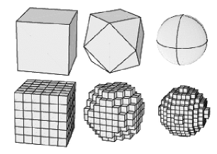
Figure 1: The “idealized” excision shapes one may wish to use for excision - a cube, a cuboctahedron, and a sphere, along with their representations on a Cartesian grid. The commonly-seen “Lego sphere” at the bottom right is the largest of the three shapes in terms of the volume it encloses.

To facilitate the excision method, we adopt the common practice of carrying an extra grid function, called the “mask”, to indicate the state of a grid-point in the computational domain. The typical states of a grid-point are: excised, excision boundary, interior, and outer boundary. Fig. 2 depicts a schematic representation of the mask variable. The large, dark circle is the location of the apparent horizon. The excision region is a “Lego sphere” represented by the thick line. The filled circles are the excision boundary points, while the empty circles are the excised points. We also use the mask function to label the outer boundary points, but this is irrelevant in the present discussion on excision.

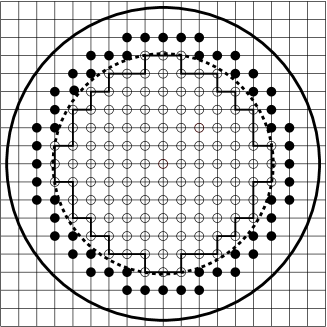
Figure 2: Schematic of the mask function for the case of spherical excision approximated on a Cartesian grid. The large, dark circle represents the location of the apparent horizon, while the light circle is the spherical excision region which is approximated by the dark line. The small, filled circles are the points on the excision boundary.

Given $u^{n}$ at the interior, excision boundary and outer boundary points, the r.h.s. $\rho$ of the evolution equations (11) for the interior grid-points are constructed and used to update $u^{n}\rightarrow u^{n+1}$ at these points. Before any subsequent updating takes place, including intermediate iterated Crank-Nicholson steps, updating of $u^{n}$ at the excision boundary is required.

Our approach for updating data at the excision boundary is designed to avoid altering the finite difference stencils used for the interior points. This is crucial for preserving a simple code. It consists of obtaining the data at the excision boundary via polynomial extrapolation. In order to simplify matters even further, we perform one-dimensional extrapolations along normal directions to the excision boundary. Because in general the excision boundary is only a discretized approximation to the geometric shape desired, the normal to the excision boundary is not aligned with the grid-points in the computational domain. We select the direction of extrapolation to be as close as possible to the direction of the normal for which all data involved on the extrapolation lie on grid-points.

We consider two approaches to construct data at the excision boundary. One approach involves the extrapolation of $\rho$ from the interior points to the excision boundary (rhs-extrapolation method). The other approach is based on extrapolation of the solution $u^{n+1}$ (sol-extrapolation method). Fig. 3 shows an illustration of both methods. Excised points are labeled with an X, the excision boundary points with a box and interior points with a solid dot. As mentioned before, for each interior point we can use centered finite differencing to calculate $\rho$. That is, $\rho_{2}$ through $\rho_{6}$ in Fig. 3 are known, but $\rho_{1}$ is unknown. The value of $\rho_{1}$ is, in principle, required to obtain $u_{1}^{n+1}$. The rhs-extrapolation method finds the value $\rho_{1}$ using the values of $\rho_{2}$ through $\rho_{5}$, depending on the order of the extrapolation.

Given that for the interior points, the truncation error in the discretizations to obtain $\rho$ is second-order, the rhs-extrapolation must be such that the overall truncation error is preserved. This implies rhs-extrapolations of at least second-order. That is,

$$\rho_{1}=2\,\rho_{2}-\rho_{3}+O(h^{2})\,,$$ (14)

with $h$ the grid spacing. It is important to notice that the simple excision method first used by Alcubierre1 and later by Yo_stable consists of first-order extrapolation, namely $\rho_{1}=\rho_{2}$. This choice yields truncation errors of $O(h)$. Our numerical experiments with a moving black hole using zero-order extrapolations quickly became unstable, in agreement with similar results in Yo_moving . A possible reason why zero-order extrapolation works for non-moving single black holes is that, from Eq. (11), the $\rho_{1}=\rho_{2}$ condition is equivalent in the continuum to

$$0=\partial_{r}\rho=\partial_{r}\partial_{t}u=\partial_{t}\partial_{r}u\,,$$ (15)

which is consistent with the time-independent nature of the solution.

The sol-extrapolation method uses the values $u_{2}^{n+1}$ through $u_{5}^{n+1}$ to obtain $u_{1}^{n+1}$, as depicted by the solid black arrow. In order to preserve second-order accuracy of the solution in this case, third-order extrapolations are needed. This is because the extrapolated value $u_{1}^{n+1}$ will be used in computing $\rho_{2}$ for the updating $u_{2}^{n+1}\rightarrow u_{2}^{n+2}$.

Figure 3: In this schematic illustration of extrapolation onto the excision boundary, an X represents an excised point, a box represents an excision boundary point, and a solid dot represents an interior point.

As the coordinate location of a black hole changes, so does the position of the excision region. We adjust the numerical evolution such that the excision region does not move by more than a grid-point. The consequences of this change of location are that points previously labeled excision boundary are now interior and points previously labeled excised are now excision boundary. Fig. 4 depicts this process. The movement is indicated by the shift in the apparent horizon (dark circles), which causes the excision region to shift in order to remain centered on the apparent horizon. The dotted circles are the original apparent horizon and excision region. The filled circles are the new excision boundary points that were previously excised points. While nothing needs to be done with interior points, we need to populate the previously excised points with values. This is done following the sol-extrapolation method previously described.

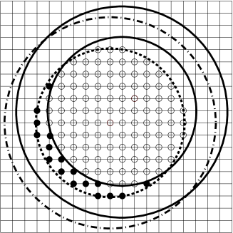
Figure 4: This figure is similar to Fig. 2; however, now the excision boundary has moved, shown here by the shift in the apparent horizon. The excision region must shift to remain centered within the apparent horizon, thus causing a need to populate previously excised points, represented here as filled circles.

IV Dancing Black Hole

In this section, we present numerical experiments that demonstrate the ability of the Maya code to handle moving excision boundaries. Because the algorithms and data structures presented here are general, they can provide a preliminary treatment for non-trivial time-dependent systems such as black-hole binaries.

In order to test our excision algorithm, we introduce the simplest time-dependency into the system that does not change the form of the metric. We consider a single, non-rotating black hole in ingoing Eddington-Finkelstein coordinates and apply a coordinate transformation of the form:

$$x^{i}\rightarrow x^{i}+d^{i}\,,$$ (16)

where

$$d^{i} = \left[A\sin\left(\frac{Vt}{A}\right),0,0\right]\;\text{or}$$ (17)

$$d^{i} = \left[A\cos\left(\frac{Vt}{A}\right),A\sin\left(\frac{Vt}{A}\right),0\right]\,.$$ (18)

Notice that this is a coordinate transformation of the spatial coordinates only. The above transformation induces the following change on the shift vector:

$$\beta^{i}\rightarrow\beta^{i}+b^{i}\,,$$ (19)

where

$$b^{i} = \left[V\cos\left(\frac{Vt}{A}\right),0,0\right]\;\text{or}$$ (20)

$$b^{i} = \left[-V\sin\left(\frac{Vt}{A}\right),V\cos\left(\frac{Vt}{A}\right),0\right]\,.$$ (21)

The functional form of $\alpha,\,g_{ij}$ and $K_{ij}$ remains the same. The only effect of this coordinate transformation is to change the coordinate location of the black hole. For the case (17), the black hole bounces back and forth with an amplitude $A$ and maximum coordinate velocity $V$ (bouncing-hole). Similarly, for the case (18), the black hole moves in a circle of radius $A$ and coordinate velocity $V$ (circling-hole).

The size of the excision region depends on the shape chosen. In the case of excising a spherical region, the excision radius was set to $1.5M$ with $M$ the mass of the black hole and $2M$ its radius, while the cubical excision region is inscribed to fit inside a sphere of radius $1.5M$. That is, we are excising a larger region of the computational domain when we use a sphere. We have empirically found that sol-extrapolation performs a little better than rhs-extrapolation for the tests under consideration. We use third-order ($O(h^{3})$) sol-extrapolation for the excision boundary and fourth-order for repopulating. The simulations were carried out with grid-spacings $h=0.2M$ and imposing equatorial symmetry about the $z$-axis. The computational domain has a total length of $20M$ in the $x$ and $y$ directions and $7M$ in the $z$ direction. We used values of $A=1.0M$ and $V=0.5$ for the simulations presented here.

The driver gauge conditions commonly used to produce long-term stability in single, non-moving black-hole evolutions are the $1+\log$ slicing and $\Gamma$-driver; that is,

$$\partial_{t}\alpha = \nabla_{i}\beta^{i}-\alpha\,K$$ (22)

$$\partial_{t}\beta^{i} = \lambda\,\partial_{t}\widehat{\Gamma}^{i}\,,$$ (23)

respectively. Unfortunately, these gauge condition do not work for our moving black-hole tests. The black-hole solution that one obtains under the coordinate transformation (16) are not compatible with these conditions. New or modified driver gauge conditions would have to be constructed. These new driver conditions would likely be dependent on the particular nature of our moving black-hole solution, thus not generalizable to astrophysically interesting cases such as black-hole binaries. Because the focus of the work in this paper is on excision, we have chosen to set $\alpha$ and $\beta^{i}$ to the analytic values given by the exact solution. It is well known that using analytic lapse and shift gauge conditions yields evolutions of single, non-moving black hole lasting $<100M$. As we will see next, the limits in duration of our moving black-hole simulations are consistent with the stationary cases.

As mentioned before, a similar problem arises with the boundary condition (13). This condition assumes that the analytic solution is time-independent. For the case of time-dependent solutions, the condition becomes

$$\partial_{t}u=\partial_{t}u_{o}-\frac{x^{i}}{r}\partial_{i}(u-u_{o})+\frac{(u-u_{o})}{r}\,.$$ (24)

The modified condition (24) should in principle work for our time-dependent case. However, one needs to remember that the outer boundary condition for the connection $\widehat{\Gamma}^{i}$ that yields long-term stability for non-moving holes was not (13), but $\partial_{t}\widehat{\Gamma}^{i}=0$. We were unable to obtain a condition applicable to our time-dependent case that would lead to significant improvements in the duration of the evolutions. Therefore, for simplicity, we have chosen instead to directly use for all fields the analytic solution as the boundary condition.

Fig. 5 is a $xt$-plot of the variable $\Phi$ for the bouncing-hole simulation. The sinusoidal flat region is a $x$-cross section of the world-tube of the excision boundary. Fig. 6 is also a $xt$-plot but in this case for the normalized Hamiltonian constraint. The reflections at the outer boundary are clear from this figure. These effects become stronger with time and eventually are one of the main causes of the simulation terminating. The other contributing factors are the analytic gauge conditions. The circling case is depicted in Fig. 7. The figure consists of stacked time slices of the variable $\Phi$. The time slices are separated by $15M$ increments in time. For clarity, the domain displayed only represents $\pm 5M$ in the $x$ and $y$ dimensions. The “orbit” of the black hole is $4\pi$, so each slice represents an evolution of approximately one and a quarter orbits from the slice preceding it. Animations of both bouncing and circling holes can be found at movies .

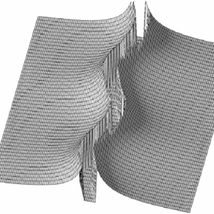
Figure 5: Space-time plot of the BSSN variable $\Phi$ for a bouncing-hole. The plot shows the evolution in the interval $0\leq t\leq 25M$. Time runs along the sinusoidal canyon.

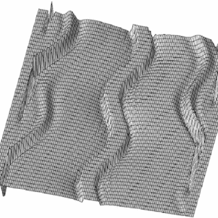
Figure 6: Space-time plot of the normalized Hamiltonian constraint for bouncing-hole. The plot shows the evolution in the interval $0\leq t\leq 25M$. Time runs along the sinusoidal canyon.

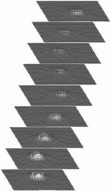
Figure 7: Stacked time slices of the BSSN variable $\Phi$ for a circling-hole, with time proceeding vertically upward, and the time slices separated by $15M$. The domain displayed only represents $\pm 5M$ in the $x$ and $y$ dimensions, for greater clarity. The “orbit” of the black hole is $4\pi$, so each slice represents an evolution of approximately one and a quarter orbits from the slice preceding it.

For comparison of evolutions, we monitor the Hamiltonian constraint, the area of the apparent horizon, and a “mass” function $M_{\Phi}$ obtained from

$$M_{\Phi}=\frac{r}{2}e^{12\Phi}-1\,.$$ (25)

For the exact solution, $M_{\Phi}$ is equal to the mass of the black hole. In all the following figures (Figs. 9-11), the top panels depict results using a spherical excision region and the bottom cubical. We also show results from a stationary black-hole case with a solid line. This is our reference case as we do not expect the moving cases to supersede the stationary case. The dotted lines represent the bouncing-hole and the dashed the circling-hole.

Fig. 9 contains plots of the L2-norm of the Hamiltonian constraint versus time for each case. It is evident from this figure that the simulation is unstable even in the case of a stationary black hole. The instability is likely due to the gauge and boundary conditions. When we turned on the driver conditions (22) and (23), as well as the boundary condition (13), long-term stable runs for a stationary hole were obtained, as one can see from Fig. 8, similar to those in Yo_stable . Fig. 10 shows the area of the apparent horizon versus time; the apparent horizon tracker is described in schnetter . The apparent horizon tracker fails to give reasonable results at approximately $t=90M$ because the coordinate distortions are such that the horizon intersects the excision region at one or more points. Finally, Fig. 11 shows plots of the L2-norm of $M_{\Phi}$ versus time. The reason why the L2-norm of $M_{\Phi}$ does not show the jagged behavior is because the L2-norm of $M_{\Phi}$ was done with data that did not include excision boundary data. The data were taken from within a shell centered at the location of the black hole a distance $0.5\,M$ from the excision boundary. The jaggedness in the Hamiltonian constraint plots is due to the artificial jump of values because the center of the excision region is forced to be at a grid point, thus producing discontinuous motion of the excision region.

Figure 8: L2-norm of the time derivative of $K$ for a single, stationary black hole with driver conditions (22-23) and boundary condition (13).

Figure 9: L2-norm of the Hamiltonian constraint. The top panel shows results when a cubical excision is used and the bottom panel corresponds to spherical excision. In each of the panels the solid line depicts data from a stationary black hole, the dotted line from a bouncing black-hole and the dashed line from a circling black-hole.

Figure 10: Same as in Fig. 9, but for the area of the black hole’s apparent horizon. For reference, the area of a single black hole is $16\,\pi\,M^{2}=50.2655\,M$.

Figure 11: Same as in Fig. 9, but for the L2-norm of the mass function $M_{\Phi}$.

V Conclusions

Ref Alcubierre1 described a simple excision algorithm that extended the lifetimes of time-independent, single black-hole evolutions. This work was expanded in Ref. Yo_moving , showing that higher order extrapolation is necessary for stability in studying the dynamics of a scalar field in the background of a boosted Kerr-Schild background. We have generalized and applied the excision algorithm presented in Yo_moving to the case of a single black hole moving its coordinate location throughout the computational domain. We showed that this algorithm is generalizable to non-stationary black-hole space-times. We also find that, despite the fact that a cubical excision region is all that is necessary for long-lived stationary black-hole runs, a spherical excision boundary is viable. A spherical shape may be more desirable in dynamic simulations because it allows the excision region to fit more easily within the apparent horizon. It is important to emphasize that the algorithm in this work for excising the black hole as it moves through the computational domain behaves in a similar way to excising a stationary black hole. This suggest that as gauge and boundary conditions suitable for time-dependent solutions are developed, the excision method discussed in this work can be directly implemented without requiring further or with minimal modifications.

VI Acknowledgments

We thank Miguel Alcubierre, Bernd Brügmann and Jorge Pullin for helpful discussions. Parallel and I/O infrastructure provided by Cactus. We acknowledge the support of the Center for Gravitational Wave Physics funded by the National Science Foundation under Cooperative Agreement PHY-0114375. Work partially supported by NSF grants PHY-9800973 to Penn State and PHY-9800737 PHY-9900672 to Cornell University.

References

- (1) L. Lehner Class. Quant. Grav. vol. 18, pp. R25-R86 (2001).
- (2) T. Baumgarte and S. Shapiro, gr-qc/0211028.
- (3) R. Gómez, L. Lehner, R. Marsa, J. Winicour, A. Abrahams, A. Anderson, P. Anninos, T. Baumgarte, N. Bishop, S. Brandt, J. Browne, K. Camarda, M. Choptuik, G. B. Cook, C. R. Evans, L. S. Finn, G. Fox, T. Haupt, M. F. Huq, L. E. Kidder, S. Klasky, P. Laguna, W. Landry, J. Lenaghan, R. Masso, R. A. Matzner, S. Mitra, P. Papadopoulos, M. Parashar, L. Rezzolla, M. E. Rupright, F. Saied, P. E. Saylor, M. A. Scheel, E. Seidel, S. L. Shapiro, D. Shoemaker, L. Smarr, B. Szilagyi, S. A. Teukolsky, M. H. P. M. van Putten, P. Walker, J. W. York Jr, Phys. Rev. Lett. vol. 80, pp. 3915-3918 (1998).
- (4) M. Alcubierre and B. Brügmann, Phys. Rev. D vol. 63, pp. 104006-104012 (2001).
- (5) L. Kidder, M. Scheel, S. Teukolsky, Phys. Rev. D vol. 64, pp. 064017-064030 (2001).
- (6) H. Yo, T. Baumgarte, S. Shapiro, Phys. Rev. D vol. 64, pp. 124011-124024 (2001).
- (7) P. Brady, J. Creighton, K. Thorne, Phys. Rev. D vol. 58, pp. 061501-061507 (1998).
- (8) R. Gómez, L. Lehner, R. Marsa, J. Winicour, Phys. Rev. D vol. 57, pp. 4778-4788 (1997).
- (9) G. Cook, M. Huq, S. Klasky, M. Scheel, A. Abrahams, A. Anderson, P. Anninos, T. Baumgarte, N. Bishop, S. Brandt, J. Browne, K. Camarda, M. Choptuik, C. Evans, L. Finn, G. Fox, R. Gómez, T. Haupt, L. Kidder, P. Laguna, W. Landry, L. Lehner, J. Lenaghan, R. Marsa, J. Masso, R. Matzner, S. Mitra, P. Papadopoulos, M. Parashar, L. Rezzolla, M. Rupright, F. Saied, P. Saylor, E. Seidel, S. Shapiro, D. Shoemaker, L. Smarr, B. Szilagyi, S. Teukolsky, M. van Putten, P. Walker, J. Winicour, J. York Jr, Phys. Rev. Lett. vol. 80, pp. 2512-2516 (1998).
- (10) S. Brandt, R. Correll, R. Gómez, M. Huq, P. Laguna, L. Lehner, P. Marronetti, R. Matzner, D. Neilsen, J. Pullin, E. Schnetter, D. Shoemaker, J. Winicour, Phys. Rev. Lett. vol. 85, pp. 5496-5499 (2000).
- (11) H. Yo, T. Baumgarte, S. Shapiro, Phys. Rev. D vol. 66, pp. 084026-084039 (2002).
- (12) R. Arnowitt, S. Deser and C.W. Misner, in Gravitation: An Introduction to Current Research, edited by L. Witten (John Wiley, New York, 1962), pp. 227-265.
- (13) J. York, in Sources of Gravitational Radiation, edited by L. Smarr (Cambridge University Press, Cambridge, 1979), pp.83-126.
- (14) M. Shibata and T. Nakamura, Phys. Rev. D vol. 52, pp. 5428-5444 (1995).
- (15) T. Baumgarte, S. Shapiro, Phys. Rev. D vol. 59, pp. 024007-024014 (1999).
- (16) B. Kelly, P. Laguna, K. Lockitch, J. Pullin, E. Schnetter, D. Shoemaker, M. Tiglio, Phys. Rev. D vol. 64, pp. 084013-084027 (2001).
- (17) S. Teukolsky Phys. Rev. D vol. 61, pp. 087501-087502 (2000).
- (18) Cactus http://www.cactuscode.org
- (19) P. Laguna and D. Shoemaker, Class. Quant. Grav. vol. 19, pp. 3679-3686 (2002).
- (20) M. Alcubierre, B. Brügmann, P. Diener, M. Koppitz, D. Pollney, E. Seidel, R. Takahashi, gr-qc/0206072.
- (21) J. Thornburg, Class. Quant. Grav. vol. 4, pp. 1119-1131 (1987).
- (22) R.W. Wald, General Relativity, The University of Chicago Press, Chicago, (1984).
- (23) O. Reula, Living Rev. in Relativity, (1998), 3, http://www.livingreviews.org/Articles/Volume1/1998-3reula.
- (24) M. Alcubierre, G. Allen, B. Brügmann, E. Seidel, W. Suen Phys. Rev. D vol. 62, pp. 124011-124026 (2000).
- (25) O. Sarbach, G. Calabrese, J. Pullin, M. Tiglio Phys. Rev. D vol. 66, pp. 064002-064009 (2002).
- (26) Animations of moving holes can be found at http://www.astro.psu.edu/nr/papers/2003/excision.
- (27) E. Schnetter, gr-qc/0206003.