Radiation from accelerated black holes in a de Sitter universe

Abstract

Radiative properties of gravitational and electromagnetic fields generated by uniformly accelerated charged black holes in asymptotically de Sitter spacetime are studied by analyzing the $C$-metric exact solution of the Einstein-Maxwell equations with a positive cosmological constant $\Lambda$. Its global structure and physical properties are thoroughly discussed. We explicitly find and describe the specific pattern of radiation which exhibits the dependence of the fields on a null direction along which the (spacelike) conformal infinity is approached. This directional characteristic of radiation supplements the peeling behavior of the fields near infinity. The interpretation of the solution is achieved by means of various coordinate systems, and suitable tetrads. The relation to the Robinson-Trautman framework is also presented.

I Introduction

There has been great effort in general relativity devoted to investigation of gravitational radiation in asymptotically flat spacetimes. Some of the now classical works, which date back to the 1960s, set up rigorous frameworks within which a general asymptotic character of radiative fields near infinity could be elucidated Bondi (1960); Bondi et al. (1962); Sachs (1962); van der Burg (1969); Newman and Penrose (1962); Newman and Unti (1962); Sachs (1961); Penrose (1965, 1964, 1967, 1963). Also, particular examples of explicit exact radiative spacetimes have been found and analyzed, e.g., Refs. Bondi et al. (1959); Ehlers and Kundt (1962); Robinson and Trautman (1962); Bonnor and Swaminarayan (1964), for a review of these important contributions to the theory of radiation see, for example, Refs. Pirani (1965); Bonnor et al. (1994); Bičák (1985, 1997, 2000).

One of the fundamental approaches to investigate the radiative properties of a gravitational field at large distances from a bounded source is based on introducing a suitable Bondi-Sachs coordinate system adapted to outgoing null hypersurfaces, and expanding the metric functions in negative powers of the luminosity distance Bondi (1960); Bondi et al. (1962); Sachs (1962); van der Burg (1969). In the case of asymptotically flat spacetimes this framework enables one to define the Bondi mass (total mass of the system as measured at future null infinity ${\mathcal{I}}^{+}$), and characterize the time evolution including radiation in terms of the news functions. Using these concepts it is possible to formulate a balance between the amount of energy radiated by gravitational waves and the decrease of the Bondi mass of an isolated system. Unfortunately, this standard explicit approach is not directly applicable to spacetimes whose conformal infinity ${\mathcal{I}}^{+}$ has a spacelike character as is the case of an asymptotically de Sitter universe which we wish to study here.

Alternatively, in accordance with the Newman-Penrose formalism Newman and Penrose (1962); Newman and Unti (1962), information about the character of radiation in asymptotically flat spacetimes can be extracted from the tetrad components of fields measured along a family of null geodesics approaching ${\mathcal{I}}^{+}$. The gravitational field is radiative if the dominant components of the Weyl tensor ${\boldsymbol{\mathbf{C}}}_{\alpha\beta\gamma\delta}$ (or of the Maxwell tensor ${\boldsymbol{\mathbf{F}}}_{\alpha\beta}$ in the electromagnetic case) fall off as ${1/\eta}$, where $\eta$ is an affine parameter along the null geodesics. The rate of approach to zero of the Weyl and electromagnetic tensor is generally given by the “peeling off” theorem of Sachs Sachs (1961, 1962); Penrose (1965). In analogy to this well-known behavior it is natural to expect that those components of the fields in parallelly transported tetrad which are proportional to ${1/\eta}$ characterize gravitational and electromagnetic radiation also in more general cases of spacetimes not asymptotically flat. We shall adopt such a definition of radiation below.

In the presence of a positive cosmological constant $\Lambda$, however, the conformal infinity ${\mathcal{I}}^{+}$ has a spacelike character, and for principal reasons the rigorous concept of gravitational and electromagnetic radiation is much less clear. As Penrose noted in the 1960s Penrose (1964, 1967) already, following his geometrical formalization of the idea of asymptotical flatness based of the conformal technique Penrose (1963, 1965), radiation is defined “less invariantly” when ${\mathcal{I}}$ is spacelike than when it has a null character.

One of the difficulties related to the spacelike character of the infinity is that initial data on ${\mathcal{I}}^{-}$ (or final data on ${\mathcal{I}}^{+}$) for, e.g., electromagnetic field with sources cannot be prescribed freely because the Gauss constraint has to be satisfied at ${\mathcal{I}}^{-}$ (or ${\mathcal{I}}^{+}$). This results in the insufficiency of purely retarded solutions in case of a spacelike ${\mathcal{I}}^{-}$ — advanced effects must also be presented. This phenomenon has been demonstrated explicitly recently Bičák and Krtouš (2001) by analyzing test electromagnetic fields of uniformly accelerated charges in de Sitter background.

We will concentrate on another crucial difference in behavior of radiative fields near null versus spacelike infinity. In the case of asymptotically flat spacetimes, any point $N_{+}$ at null infinity ${\mathcal{I}}^{+}$ can be approached essentially only along one null direction. However, if future infinity ${\mathcal{I}}^{+}$ has a spacelike character, one can approach the point $N_{\scriptscriptstyle{\boldsymbol{+}}}$ from infinitely many different null directions. It is not a priori clear how the radiation components of the fields depend on a direction along which $N_{\scriptscriptstyle{\boldsymbol{+}}}$ is approached. In this paper such dependence will be thoroughly investigated.

In fact, radiative properties of a test electromagnetic field of two uniformly accelerated point-like charges in the de Sitter background has recently been studied Bičák and Krtouš (2002); Bičák and Krtouš . Within this context, the above mentioned directional dependence has been explicitly found. In particular, it has been demonstrated that there are always exactly two special directions — those opposite to the direction from the sources — along which the radiation vanishes. For all other directions the radiation is nonvanishing and it is described by an explicit formula which completely characterizes its angular dependence.

In the present paper, these results will be considerably generalized to both gravitational and electromagnetic field which are not just test fields in the de Sitter background. Interestingly, it will be demonstrated that the gravitational and electromagnetic fields of the $C$-metric with ${\Lambda>0}$, which is an exact solution representing a pair of uniformly accelerated possibly charged black holes in the de Sitter-like universe, exhibits exactly the same asymptotic radiative behavior as the test fields Bičák and Krtouš (2002); Bičák and Krtouš . We are thus able to supplement the information about the peeling behavior of the fields near ${\mathcal{I}}^{+}$ with an additional general property of radiation, namely with the specific directional pattern of the radiation at conformal infinity.

The $C$-metric with ${\Lambda=0}$ is a well-known solution of the Einstein(-Maxwell) equations which, together with the famous Bonnor-Swaminarayan solutions Bonnor and Swaminarayan (1964), belongs to a large class of asymptotically flat spacetimes with boost and rotational symmetry Bičák and Schmidt (1989) representing accelerated sources. It was discovered already in 1917 by Levi-Civita Levi-Civita (1917) and Weyl Weyl (1918), and named by Ehlers and Kundt Ehlers and Kundt (1962). Physical interpretation and understanding of the global structure of the $C$-metric as a spacetime with radiation generated by a pair of accelerated black holes came with the fundamental papers by Kinnersley and Walker Kinnersley and Walker (1970) and Bonnor Bonnor (1983). Consequently, a great number of works analyzed various aspects and properties of this solution, including its generalization which admits a rotation of the black holes. References and summary of the results can be found, e.g., in Refs. Bičák and Schmidt (1989); Bičák and Pravda (1999); Letelier and Oliveira (2001); Pravda and Pravdová (2000). Another possible generalization of the standard $C$-metric exists, namely, that to a nonvanishing value of the cosmological constant $\Lambda$ Plebański and Demiański (1976), cf.  Carter (1968); Debever (1971). However, in this case a complete understanding of global properties, mainly a character of radiation, is still missing despite a successful application of this solution to the problem of cosmological production of black holes Mann and Ross (1995), and its recent analysis and interpretation Podolský and Griffiths (2001); Dias and Lemos (a, b).

There exists a strong motivation to investigate the $C$-metric solution with ${\Lambda>0}$. As will be demonstrated below, it may serve as an interesting exact model of gravitational and electromagnetic radiation of bounded sources in the asymptotically de Sitter universe (in contrast to ${\Lambda=0}$, in which case the system is not permanently bounded). The character of radiation, in particular the above mentioned dependence of the asymptotic fields on directions, along which points on the de Sitter-like infinity ${\mathcal{I}}^{+}$ are approached, can explicitly be found and studied. These results may provide an important clue to formulation of a general theory of radiation in spacetimes which are not asymptotically flat. In addition to this purely theoretical motivation, understanding the behavior of accelerated black holes in the universe with a positive value of the cosmological constant can also be interesting from perspective of contemporary cosmology.

The paper is organized as follows. First, in Section II we present the $C$-metric solution with a positive cosmological constant in various coordinates which will be necessary for the subsequent analysis. The global structure of the spacetime is described in detail in Section III. Next, in Section IV we introduce and discuss various privileged orthonormal and null tetrads near the de Sitter-like infinity ${\mathcal{I}}^{+}$ together with their mutual relations, and we give corresponding components of the gravitational and electromagnetic $C$-metric fields. Section V contains the core of our analysis. We carefully define interpretation tetrad parallelly transported along all null geodesics approaching asymptotically a given point on spacelike ${\mathcal{I}}^{+}$ from different spatial directions. The magnitude of the leading terms of gravitational and electromagnetic fields in such a tetrad then provides us with a specific directional pattern of radiation which is described and analyzed. This result is subsequently rederived in Section VI using the Robinson-Trautman framework which also reveals some other aspects of the radiative properties. Particular behavior of radiation along the algebraically special null directions is studied in Section VII. For these privileged geodesics the results are obtained explicitly without performing asymptotic expansions of the physical quantities near ${{\mathcal{I}}^{+}}$. In this case we also study a specific dependence of the field components on a choice of initial conditions on horizons.

The paper contains four appendixes. Appendix A summarizes known and also several new coordinates for the $C$-metric with ${\Lambda>0}$. The properties of the specific metric functions are described in Appendix B. In Appendix C useful relations between the various coordinate 1-form and vector frames are presented, together with the relations between the different privileged null tetrads. Appendix D contains general Lorentz transformations of the null tetrad components of the gravitational and electromagnetic fields.

II The $C$-metric with a cosmological constant in suitable coordinates

The generalization of the $C$-metric which admits a nonvanishing cosmological constant ${\Lambda>0}$, representing a pair of uniformly accelerated black holes in a “de Sitter background”, has the form

$${\boldsymbol{g}}=\frac{1}{A^{2}(x+y)^{2}}\Bigl{(}-F\,\mathbf{d}t^{2}+\frac{1}{F}\,\mathbf{d}y^{2}+\frac{1}{G}\,\mathbf{d}x^{2}+G\,\mathbf{d}\varphi^{2}\Bigr{)}{\mbox{\;,}}$$ (1)

where

$$F =-\frac{1}{a_{\scriptscriptstyle\Lambda}^{2}A^{2}}-1+y^{2}-2mA\,y^{3}+e^{2}A^{2}\,y^{4}{\mbox{\;,}}$$ (2)

$$G =\mspace{81.0mu}1-x^{2}-2mA\,x^{3}-e^{2}A^{2}\,x^{4}{\mbox{\;,}}$$

see Eqs. (126), (127). Here ${t\in{\mathbb{R}}}$, ${\varphi\in(-\pi C,\pi C)}$, $m$, $e$, $A$, $C$ are constants, and ranges of the coordinates ${x,\,y}$ (or, more precisely, of the related coordinates ${\xi,\,\upsilon}$ defined below by Eq. (7)) will be discussed in detail in the next section. For convenience, we have parametrized the cosmological constant $\Lambda$ by the “de Sitter radius” as

$$a_{\scriptscriptstyle\Lambda}=\sqrt{\frac{3}{\Lambda}}{\mbox{\;.}}$$ (3)

The metric (1) is a solution of the Einstein-Maxwell equations with the electromagnetic field given by (note nt:Units )

$${\boldsymbol{\mathbf{F}}}=e\,\mathbf{d}y\wedge\mathbf{d}t{\mbox{\;.}}$$ (4)

The constants $m$, $e$, $A$, and $C$ parametrize mass, charge, acceleration, and conicity of the black holes, although their relation to physical quantities is not, in general, direct. For example, the total charge $Q$ on a timelike hypersurface ${t=\text{constant}}$ localized inside a surface ${y=\text{constant}}$, defined using the Gauss law, is given by ${Q=\frac{1}{2}(\xi_{2}-\xi_{1})\,Ce}$, where the constants ${\xi_{1},\,\xi_{2}}$ are introduced at the beginning of the next section. Obviously, $Q$ depends not only on the charge parameter $e$. Similarly, physical conicity is proportional to the parameter $C$, but it also depends on other parameters, see Eq. (20) below. The concept of mass (outside the context of asymptotically flat spacetimes) and of physical acceleration of black holes is even more complicated. We will return to this point at the end of the next section. For satisfactory interpretation of the parameters $m$, $e$, and $A$ in the limit of their small values see, e.g., Ref. Podolský and Griffiths (2001).

In the following we will always assume

$$m>0{\mbox{\;,\quad}}e^{2}<m^{2}{\mbox{\;,\quad}}A>0{\mbox{\;,}}$$ (5)

and $F$, as a polynomial in $y$, to have only distinct real roots. Also, instead of the acceleration constant $A$ we will conveniently use the dimensionless acceleration parameter $\alpha$ defined as

$$\sinh\alpha=a_{\scriptscriptstyle\Lambda}A{\mbox{\;,\quad}}\cosh\alpha=\sqrt{1+a_{\scriptscriptstyle\Lambda}^{2}A^{2}}{\mbox{\;.}}$$ (6)

We will also use other suitable coordinates which are introduced and discussed in more detail in Appendix A. Here we list only the basic definitions and the corresponding forms of metric.

The rescaled coordinates ${\tau,\,\upsilon,\,\xi,\,\varphi}$ are defined

$$\tau =\,t\,\coth\alpha{\mbox{\;,}} \varphi =\varphi{\mbox{\;,\quad}}$$ (7)

$$\upsilon =y\,\tanh\alpha{\mbox{\;,\quad}} \xi =-x{\mbox{\;,}}$$

cf.  Eq. (130), in which the metric takes the form (131),

$${\boldsymbol{g}}=r^{2}\Bigl{(}-{\mathcal{F}}\,\mathbf{d}\tau^{2}+\frac{1}{{\mathcal{F}}}\,\mathbf{d}\upsilon^{2}+\frac{1}{{\mathcal{G}}}\,\mathbf{d}\xi^{2}+{\mathcal{G}}\,\mathbf{d}\varphi^{2}\Bigr{)}{\mbox{\;,}}$$ (8)

where

$$r=\frac{1}{A(x+y)}=\frac{a_{\scriptscriptstyle\Lambda}}{\upsilon\cosh\alpha-\xi\sinh\alpha}{\mbox{\;,}}$$ (9)

and

$$-{\mathcal{F}} =1-\upsilon^{2}+\cosh\alpha\,\frac{2m}{a_{\scriptscriptstyle\Lambda}}\;\upsilon^{3}-\cosh^{2}\alpha\,\frac{e^{2}}{a_{\scriptscriptstyle\Lambda}^{2}}\;\upsilon^{4}{\mbox{\;,}}$$ (10)

$${\mathcal{G}} =1-\xi^{2}+\sinh\alpha\,\frac{2m}{a_{\scriptscriptstyle\Lambda}}\;\xi^{3}-\sinh^{2}\alpha\,\frac{e^{2}}{a_{\scriptscriptstyle\Lambda}^{2}}\;\xi^{4}{\mbox{\;.}}$$

The coordinates ${\omega,\,\tau,\,\sigma,\,\varphi}$ adapted to the Killing vectors ${{\boldsymbol{\mathbf{\partial}}}_{\tau}}$, ${{\boldsymbol{\mathbf{\partial}}}_{\varphi}}$ and the conformal infinity ${\mathcal{I}}$ (${\omega=0}$) are defined by

$$\begin{gathered}\omega=-\upsilon\cosh\alpha+\xi\sinh\alpha{\mbox{\;,}}\\ \mathbf{d}\sigma=\frac{\sinh\alpha}{{\mathcal{F}}}\,\mathbf{d}\upsilon+\frac{\cosh\alpha}{{\mathcal{G}}}\,\mathbf{d}\xi{\mbox{\;,}}\end{gathered}$$ (11)

cf. Eqs. (146), (147), and the metric is (148),

$${\boldsymbol{g}}=\frac{a_{\scriptscriptstyle\Lambda}^{2}}{\omega^{2}}\Bigl{(}-{\mathcal{F}}\,\mathbf{d}\tau^{2}+\frac{1}{{\mathcal{E}}}\,\mathbf{d}\omega^{2}+\frac{{\mathcal{F}}{\mathcal{G}}}{{\mathcal{E}}}\,\mathbf{d}\sigma^{2}+{\mathcal{G}}\,\mathbf{d}\varphi^{2}\Bigr{)}{\mbox{\;,}}$$ (12)

where

$${\mathcal{E}}={\mathcal{F}}\cosh^{2}\alpha+{\mathcal{G}}\sinh^{2}\alpha{\mbox{\;.}}$$ (13)

Finally, we will also use the $C$-metric expressed in the Robinson-Trautman coordinates ${\zeta,\,\bar{\zeta},\,u,\,r}$ which has the form (154) (see note nt:SymTensProd for a definition of the symmetric product $\mathbin{\scriptstyle{\vee}}$)

$${\boldsymbol{g}}=\frac{r^{2}}{P^{2}}\,\mathbf{d}\zeta\mathbin{\scriptstyle{\vee}}\mathbf{d}\bar{\zeta}-\mathbf{d}u\mathbin{\scriptstyle{\vee}}\mathbf{d}r-H\,\mathbf{d}u^{2}{\mbox{\;,}}$$ (14)

with

$$\frac{1}{P^{2}}={\mathcal{G}}{\mbox{\;,\quad}}H=\frac{r^{2}}{a_{\scriptscriptstyle\Lambda}^{2}}\,{\mathcal{E}}{\mbox{\;.}}$$ (15)

It follows immediately from Eqs. (9) and (11) that

$$r=-\frac{a_{\scriptscriptstyle\Lambda}}{\omega}{\mbox{\;.}}$$ (16)

For explicit definitions of the coordinates $u$, $\zeta$ and further details see Eqs. (150), (153), and related text in Appendix A.

III The global structure

In this section we shall describe the global structure of the $C$-metric with ${\Lambda>0}$. In particular, we shall analyze the character of infinity, singularities, and possible horizons. (Cf. recent work Dias and Lemos (b) for similar discussion that covers also cases not studied here.) From the form (8) of the metric we observe that it is necessary to investigate zeros of the metric functions ${\mathcal{F}}$ and ${\mathcal{G}}$ given by Eq. (10). We will only discuss the particular case when the function ${\mathcal{F}}$ has $n$ distinct real roots, where $n$ is the degree of polynomial dependence of ${\mathcal{F}}$ on $\upsilon$ (${n=4}$ for ${e\neq 0}$). Let us denote these roots as $\;\upsilon_{\mathrm{i}}$, $\upsilon_{\mathrm{o}}$, $\upsilon_{\mathrm{c}}$, and $\;\upsilon_{\mathrm{m}}\;$ in a descending order (the meaning of the subscripts will be explained below). In the case ${e=0}$, the value of $\upsilon_{\mathrm{i}}$ is not defined, etc. Analogously, we denote the roots of ${\mathcal{G}}$ as $\xi_{1}$, $\xi_{2}$, $\xi_{3}$, and $\xi_{4}$ in an ascending order. Similarly to discussion of the $C$-metric with vanishing $\Lambda$ Kinnersley and Walker (1970); Bičák and Pravda (1999); Letelier and Oliveira (2001), the zeros of the function ${\mathcal{F}}$ correspond to horizons, and the zeros of ${\mathcal{G}}$ to axes of $\varphi$ symmetry. Following these works, and Ref. Podolský and Griffiths (2001) for ${\Lambda>0}$ in particular, the qualitative diagrams of the ${\xi{\text{-}}\upsilon}$ slice (i.e., ${\tau,\,\varphi=\text{constant}}$) are drawn in Fig. 1. In this diagram we use relations

$$\upsilon_{\mathrm{m}}\coth\alpha<\xi_{1}<0<\xi_{2}<\upsilon_{\mathrm{c}}\coth\alpha{\mbox{\;,}}$$ (17)

which are obvious from Fig. 9 in Appendix B. Different columns and rows in the diagrams in Fig. 1 correspond to different signs of the functions ${\mathcal{G}}$ and ${\mathcal{F}}$. The metric has a physical signature ${({-}{+}{+}{+})}$ for ${\xi_{1}<\xi<\xi_{2}}$ and ${\xi_{3}<\xi<\xi_{4}}$. We will be interested only in the first region.

Infinity ${\mathcal{I}}$ of the spacetime corresponds to ${r=\infty}$, or equivalently to

$$\omega=0{\mbox{\;,\quad}}\text{i.e.,}\quad\upsilon=\xi\tanh\alpha{\mbox{\;,}}$$ (18)

(double line in Fig. 1). We will restrict to the region ${\upsilon>\xi\tanh\alpha}$ (i.e., ${r>0}$) which describes both interior and exterior of accelerated black holes in de Sitter-like spacetime (the shaded areas in Fig. 1). The metric has an unbounded curvature for ${r=0}$ which corresponds to a physical singularity inside the black holes, a zig-zag line on the boundary of the diagrams in Fig. 1, in particular of the column ${\xi_{1}<\xi<\xi_{2}}$.

For a further discussion of the global structure we employ the double null coordinates ${{\tilde{u}},\,{\tilde{v}},\,\xi,\,\varphi}$ defined by Eqs. (163), (158), (159) in which the metric is (164),

$${\boldsymbol{g}}=r^{2}\Bigl{(}\frac{2\,\delta^{2}{\mathcal{F}}}{\sin{\tilde{u}}\sin{\tilde{v}}}\,\mathbf{d}{\tilde{u}}\mathbin{\scriptstyle{\vee}}\mathbf{d}{\tilde{v}}+\frac{1}{{\mathcal{G}}}\,\mathbf{d}\xi^{2}+{\mathcal{G}}\,\mathbf{d}\varphi^{2}\Bigr{)}{\mbox{\;.}}$$ (19)

Using these coordinates we can draw the conformal diagram of the spacetime section ${\tau{\text{-}}\upsilon}$, i.e., for ${\xi,\,\varphi=\text{constant}}$ — see Fig. 2. The domains I–IV in this figure correspond to the regions I–IV in Fig. 1.

The region I describes the domain of spacetime above the cosmological horizons given by ${\upsilon=\upsilon_{\mathrm{c}}}$, which has a similar structure as an analogous domain in the de Sitter spacetime. The region II corresponds to a static spacetime domain between the cosmological horizon and the (outer) horizon of the black hole. If the black hole is charged (${e\neq 0}$), region III corresponds to a spacetime domain between the outer horizon ${\upsilon=\upsilon_{\mathrm{o}}}$ and the inner horizon ${\upsilon=\upsilon_{\mathrm{i}}}$, and region IV to a domain below the inner horizon of the black hole (similar to the analogous domains of the Reissner-Nordström spacetime). The domain IV contains a timelike singularity at ${\upsilon=\infty}$ (${r=0}$). In the uncharged case (${e=0}$, ${m\neq 0}$) there is only region III which corresponds to a domain below the single black hole horizon ${\upsilon=\upsilon_{\mathrm{o}}}$. In this case the singularity at ${\upsilon=\infty}$ has a spacelike character, similarly as for the Schwarzschild black hole. If both ${e=0}$, ${m=0}$, we obtain de Sitter spacetime expressed in accelerated coordinates. In this case there is no black hole horizon, and region II (the domain below the cosmological horizon ${\upsilon_{\mathrm{c}}}$) is “cut off” by nonsingular poles ${\upsilon=\infty}$. We will return to this particular case at the end of this section.

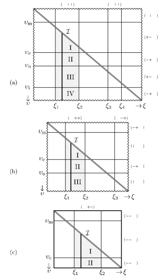
Figure 1: A qualitative diagram of the ${\xi{\text{-}}\upsilon}$ section (${\tau,\,\varphi}=\text{constant}$) of the studied spacetime. The three cases correspond to (a) charged accelerated black holes in asymptotically de Sitter universe (${e\neq 0}$, ${m\neq 0}$), (b) uncharged black holes (${e=0}$, ${m\neq 0}$), and (c) de Sitter universe (${e=0}$, ${m=0}$). Horizontal lines indicate the horizons, vertical lines are axes of $\varphi$ symmetry. The diagonal double line ${\upsilon=\xi\tanh\alpha}$ corresponds to infinity ${\mathcal{I}}$. Singularities are depicted by “zig-zag” lines. The boundary of each diagram corresponds to ${\xi,\,\upsilon=\pm\infty}$. Mutual intersections of different lines are governed by relations (17). Different columns and rows correspond to different signs of the functions ${\mathcal{G}}$ and ${\mathcal{F}}$, respectively, and thus to different signatures of the metric, which are indicated on the sides of the diagrams. The metric (8) describes, in general, four distinct spacetimes — the domains in columns ${\xi_{1}<\xi<\xi_{2}}$ and ${\xi_{3}<\xi<\xi_{4}}$, separated in addition by the infinity (the diagonal line). In this paper we discuss only the physically most reasonable spacetime with the coordinates ${\xi,\,\upsilon}$ in the ranges ${\xi_{1}<\xi<\xi_{2}}$ and ${\upsilon>\xi\tanh\alpha}$ (the shaded areas). Sections ${\xi=\text{constant}}$ which correspond to the conformal diagrams in Fig. 2 are indicated by thick lines.

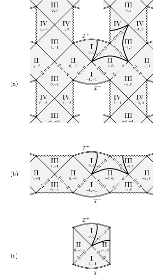
Figure 2: The conformal diagrams of the ${\tau{\text{-}}\upsilon}$ section (${\xi,\varphi}=\text{constant}$). Similarly to Fig. 1, the three diagrams correspond to the cases of (a) charged accelerated black holes, (b) uncharged black holes, and (c) de Sitter universe (in accelerated coordinates). The conformal infinities ${\mathcal{I}}$ are indicated by double lines, the singularities are drawn by “zig-zag” lines, and horizons by thin lines. The horizons ${\upsilon=\upsilon_{\mathrm{c}},\,\upsilon_{\mathrm{o}},\,\upsilon_{\mathrm{i}}}$ correspond to the values ${{\tilde{u}}=m\pi}$ or ${{\tilde{v}}=n\pi}$, ${m,n\in{\mathbb{Z}}}$. Thus, the integers ${(m,\,n)}$, indicated in the figure, label different blocks ${{\tilde{u}}\in(m\pi,(m+1)\pi)}$, ${{\tilde{v}}\in(n\pi,(n+1)\pi)}$ of the conformal diagrams. There are four types of these blocks, labeled by I–IV, which correspond to the regions I–IV in Fig. 1. The sections ${\tau=\text{constant}}$ (drawn in Fig. 1) are indicated by thick lines. Similar lines could, of course, be drawn also in other blocks. Only a part of the complete conformal diagram is shown in the cases (a) and (b), however, the rest of the diagram would have a similar structure as the part shown. The complete diagram depends on a freedom in the choice of a global topology of the spacetime given by identifications of different blocks of the conformal diagram. In the case (c), the diagram does not contain any black hole — it is “closed on its sides” by poles of a spacelike section $S^{3}$ of de Sitter universe (see the discussion at the end of Section III).

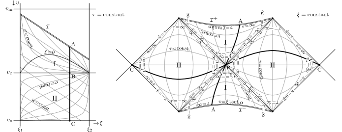
Figure 3: The ${\xi{\text{-}}\upsilon}$ (left) and the conformal (right) diagrams near infinity ${\mathcal{I}}$. Only one asymptotically de Sitter-like region of the spacetime (domains I and II of Figs. 1 and 2) is shown. Ranges of various coordinates introduced in the paper are indicated (orientation of the coordinate labels suggests a direction in which the coordinates increase). The thick line in the conformal diagram corresponds to the ${\xi{\text{-}}\upsilon}$ diagram and vice versa. In the ${\xi{\text{-}}\upsilon}$ diagram the lines of constant $\omega$ and $\sigma$ are also drawn. The coordinates ${\omega,\,\sigma}$ are not unambiguous in the full domain I, however, they are invertible near ${\mathcal{I}}$, in the domain ${{\mathcal{E}}<0}$. On the boundary ${{\mathcal{E}}=0}$ (shown in diagram) the coordinates ${\omega,\,\sigma}$ change their timelike/spacelike character. (Notice the difference between the null coordinate $v$ — diagonal straight lines — and the “radial” coordinate $\upsilon$ — curved lines — in the ${\tau{\text{-}}\upsilon}$ conformal diagram.)

Before we proceed to discuss further properties in detail let us note that (as will be explicitly demonstrated in the next section) the $C$-metric is the Petrov type $D$ spacetime, i.e., it admits two double principal null directions. These directions lie exactly in the section ${\tau{\text{-}}\upsilon}$ depicted in Fig. 2.

In this paper we are mainly interested in a behavior of fields near the infinity. Therefore, we will concentrate mostly on the region I. This region has similar properties for all possible values of the parameters $m$, $e$, and $\alpha$. Its more precise diagrams are drawn in Fig. 3. Observers in one of the regions I (near the future infinity ${\mathcal{I}}^{+}$) will consider themselves to live in an asymptotically de Sitter-like universe “containing” two causally disconnected black holes (for ${m\neq 0}$). Here by two black holes we understand those black holes (i.e., regions III and IV) immediately “visible” from the given asymptotical region I, although the geodesically complete spacetime can, of course, contain an infinite number of black holes. As we have said, the conformal infinity ${\mathcal{I}}$ is given by the condition (18), ${\omega=0}$. Thanks to a timelike character of ${\mathbf{d}\omega}$ at ${\omega=0}$ (cf.  Eq. (12)) the infinity has indeed a spacelike character as for de Sitter universe (see Refs. Penrose (1964, 1965); Penrose and Rindler (1984) for a general discussion of conformal infinity). In Fig. 1 the infinity corresponds to the diagonal line, in Fig. 2, however, it obtains a richer structure. It comprises of two parts — future infinity ${\mathcal{I}}^{+}$ and the past infinity ${\mathcal{I}}^{-}$ — both possibly consisting of several disjoint parts (depending on the global topology) in different asymptotically de Sitter domains I. Because the conformal diagrams in Fig. 2 are slices with a fixed coordinate $\xi$, and the condition (18) depends on $\xi$, the conformal infinity ${\mathcal{I}}$ would have a different position in diagrams with different values of $\xi$. We shall return to this fact at the end of this section. Note, that for values of the coordinate $\upsilon$ smaller than $\,{\xi_{2}\tanh\alpha}$, the hypersurface ${\upsilon=\text{constant}}$ reaches ${\mathcal{I}}$. Clearly, the coordinate $\upsilon$ is not well adapted to the region near the conformal infinity ${\mathcal{I}}$. Near the infinity it is more convenient to use the coordinates ${\omega,\,\tau,\,\sigma,\,\varphi}$ defined by Eqs. (11) (cf.  Eqs. (146), (147); see also Fig. 3).

The coordinate $\tau$ is a coordinate along the “boost” Killing vector ${{\boldsymbol{\mathbf{\partial}}}_{\tau}}$, and in region I it can be understood simply as a translational spatial coordinate. The coordinates ${\xi,\,\varphi}$ play roles of longitudinal and latitudinal coordinates of a suitably defined hypersurface at an “instant of time”. For example, in region I the spacelike hypersurface ${\upsilon=\text{constant}}$ has topology ${{\mathbb{R}}\times S^{2}}$ (if it does not cross infinity ${\mathcal{I}}$) with the coordinate $\tau$ along the ${\mathbb{R}}$ direction, and ${\xi,\,\varphi}$ on the sphere $S^{2}$. To justify the “longitudinal” character of the coordinate $\xi$, we introduce, instead of $\xi$, an angular coordinate $\vartheta$ by the relation ${\sin\vartheta=\sqrt{{\mathcal{G}}}}$ (cf.  Eq. (135)). This is a longitudinal angle measured by a circumference of the $\varphi$-circle (see the metric (8)). Alternatively, we can introduce the angle $\Theta$, defined by Eq. (137), measured by the length of a “meridian”. At infinity ${\mathcal{I}}$ or, in general, on any hypersurface ${\omega=\text{constant}}$, the coordinate lines ${\sigma=\text{constant}}$ coincide with the lines of constant $\xi$. The coordinate $\sigma$ thus also parametrizes the longitudinal direction near the infinity, similarly to the coordinate $\xi$.

In Section II we mentioned that the coordinate $\varphi$ along the second Killing vector ${{\boldsymbol{\mathbf{\partial}}}_{\varphi}}$ takes values in the interval $(-\pi C,\pi C)$. Here ${C>0}$ is the parameter which allows us to change the conicity on the axis of the $\varphi$ symmetry, i.e., it allows us to choose a deficit (or excess) angle around the axis arbitrarily. Such a change of the range of the coordinate $\varphi$ is allowed for any axially symmetric spacetime. The range is usually chosen in such a way that the axis of the $\varphi$ symmetry is regular. However, for the $C$-metric such a choice is not globally possible. In this case the axis consists of two parts ${\xi=\xi_{1}}$ and ${\xi=\xi_{2}}$ — one of them joins the “north” poles of the black holes, the other one joins the “south” poles. The physical conicity (defined as a limiting ratio of “circumference” and ${2\pi\!\times\!\text{``radius''}}$ of a small circle around the axis) calculated at the axes ${\xi_{1}}$ and ${\xi_{2}}$ is

$$\kappa_{1}={\textstyle\frac{1}{2}}\,C\,{\mathcal{G}}^{\prime}|_{\xi=\xi_{1}}{\mbox{\;,\quad}}\kappa_{2}=-{\textstyle\frac{1}{2}}\,C\,{\mathcal{G}}^{\prime}|_{\xi=\xi_{2}}{\mbox{\;,}}$$ (20)

respectively, see, e.g., Ref. Podolský and Griffiths (2001). In general, the values of ${\left\lvert{\mathcal{G}}^{\prime}\right\rvert}$ at ${\xi_{1}}$ and ${\xi_{2}}$ are not the same, cf.  Eq. (21) below. Therefore we can set ${\kappa=1}$ (zero deficit of angle, i.e., a regular axis) by a suitable choice of the parameter $C$ only at one part of the axis.

This fact has a clear physical interpretation. The axis with nonregular conicity corresponds to a cosmic string which causes the “accelerated motion” of the black holes. The cosmic string Vilenkin and Shellard (1994) is a one-dimensional object, sort of a “rod” or a “spring”, which is characterized by its mass density equal to its linear tension. These parameters are proportional to the deficit angle, namely, a string with a deficit angle (${\kappa<1}$) has a positive mass density and it is stretched, a string with an excess angle (${\kappa>1}$) has negative mass density and is squeezed. In Appendix B, Eq. (174), we prove for ${m\neq 0}$, ${A\neq 0}$ that

$$\kappa_{2}<\kappa_{1}{\mbox{\;.}}$$ (21)

Using this fact, we may conclude that by eliminating a nontrivial conicity at the axis ${\xi=\xi_{2}}$ (so that ${\kappa_{2}=1}$) we obtain ${\kappa_{1}>1}$, i.e., a squeezed cosmic string at the axis ${\xi=\xi_{1}}$. Alternatively, if we set the physical conicity ${\kappa_{1}=1}$ at ${\xi=\xi_{1}}$, we obtain ${\kappa_{2}<1}$, i.e., a stretched cosmic string at the axis ${\xi=\xi_{2}}$. In both these cases, as well as in the general cases of cosmic strings on both parts of the axis, the system of black holes with string(s) between them is not in an equilibrium. The string(s) acts on both black holes and cause what we usually call an “accelerated motion” of black holes. However, the precise interpretation of acceleration is not so straightforward.

The problem here is that we consider a fully self-gravitating system, not just a motion of test particles on a fixed background. The motion of black holes is actually realized through a nonstatic, nonspherical deformation of geometry of the spacetime in a direction of motion, i.e., along the axis of $\varphi$ symmetry. Moving black holes together with the cosmic string(s) curve the spacetime in such a way that, strictly speaking, it is not justified to use the term acceleration in a rigorous sense. This has several reasons. First, black holes are nonlocal objects and one can hardly expect a uniquely defined acceleration for such extended objects. Secondly, thanks to the equivalence principle we cannot distinguish between acceleration of the black holes with respect to the universe, and acceleration due to the gravitational field of each hole. Finally, one has to expect a gravitational dragging of local inertial frames by moving black holes, i.e., it is not obvious how to define an acceleration of black holes with respect to these frames. A plausible definition could be given if some privileged cosmological coordinate system playing a role of “nonmoving” background is available. Unfortunately, we are not aware of such a system applicable in a general case. In the next paragraph we shall demonstrate this approach just for a simple case of empty de Sitter spacetime. Summarizing, it is not straightforward to define the acceleration of black holes in the general case. One usually identifies the acceleration only in an appropriate limiting regime. The usage of the term acceleration for the parameter $A$ in the $C$-metric (see Refs. Bonnor (1983); Bičák and Pravda (1999); Letelier and Oliveira (2001) for the case ${\Lambda=0}$, and, e.g., Refs. Podolský and Griffiths (2001) for the case ${\Lambda\neq 0}$) has been justified exactly in this way.

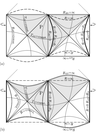
Figure 4: Conformal diagrams of de Sitter universe (a) in the standard cosmological coordinates (145), and (b) based on the accelerated coordinates (22) (cf. Eq. (137)). In contrast to Fig. 2(c), the diagram (b) depicts two sections of constant $\xi$, namely ${\xi=\xi_{1}}$ (${\Theta=0}$) at the right half of the diagram, and ${\xi=\xi_{2}}$ (${\Theta=\pi}$) at the left half. We can see that the position of infinity (double line) is different for these two values of $\xi$. For intermediate values of $\xi$ infinity ${\mathcal{I}}$ would attain an intermediate position at $\,{R=a_{\scriptscriptstyle\Lambda}/\xi\,\coth\alpha}\,$, according to Eq. (18). The infinity has a simple shape in diagram (a), where it is indicated by the horizontal lines ${R_{\scriptscriptstyle{\mathrm{dS}}}=\infty}$. In both diagrams the left and right boundaries are identified — they correspond to one of the two poles of the appropriate coordinates (the other pole is located in the center of the diagram). A horizontal line thus corresponds to the main circle of a spatial $S^{3}$ section of de Sitter universe. Bold lines corresponds to the origins of the accelerated coordinates (${R=0}$) which have been employed in the paper as “remnants” of the sources. In diagram (a) they move with respect to the cosmological frame. Diagram (b) is adapted to their accelerated motion and therefore the sources are located at origins. Dashed line corresponds to value ${R=\infty}$, i.e., ${\upsilon=0}$, where the accelerated coordinates are not well defined. Relative position of the hypersurface ${R=\infty}$ and of infinity ${R_{\scriptscriptstyle{\mathrm{dS}}}=\infty}$ can be visualized with help of a conformally related Minkowski space (lower half indicated by the shaded domain P, the upper half indicated by dotted line). In this space the infinity corresponds to hypersurface ${{\mathfrak{t}}=0}$, the coordinate singularity ${R=\infty}$ corresponds to ${{\mathfrak{t}}^{\prime}=0}$, where ${\mathfrak{t}}$ and ${\mathfrak{t}}^{\prime}$ are Minkowski time coordinates in inertial frames moving with relative velocity ${\tanh\alpha}$ — see Appendix A for a related discussion.

Of course, the situation extremely simplifies in the case of vanishing mass and charge (${m=0}$, ${e=0}$). In this case there are no black holes, and the spacetime reduces to de Sitter universe. However, if we still keep ${A\neq 0}$, a trace of (now vanished) “accelerated” sources remains in the metric (8) through the parameter $\alpha$. By a simple transformation (137),

$$T=a_{\scriptscriptstyle\Lambda}\,\tau{\mbox{\;,\quad}}R=\frac{a_{\scriptscriptstyle\Lambda}}{\upsilon}{\mbox{\;,\quad}}\cos\Theta=-\xi{\mbox{\;,\quad}}\Phi=\varphi{\mbox{\;,}}$$ (22)

we obtain the metric (142) of the de Sitter space in accelerated coordinates ${T,\,R,\,\Theta,\,\Phi}$ introduced in Ref. Podolský and Griffiths (2001) and discussed in Ref. Bičák and Krtouš . These coordinates are analogue of the Rindler coordinates in Minkowski space generalized to the case of the de Sitter universe. They are adapted to accelerated observers: the origins ${R=0}$ represent two uniformly accelerated observers which are decelerating from antipodal poles of the spherical space section of the de Sitter universe toward each other until the moment of minimal contraction of the universe, and then accelerate away back to the antipodal poles (see Fig. 4). In the standard de Sitter static coordinates ${T_{\scriptscriptstyle{\mathrm{dS}}},\,R_{\scriptscriptstyle{\mathrm{dS}}},\,\Theta_{\scriptscriptstyle{\mathrm{dS}}},\,\Phi_{\scriptscriptstyle{\mathrm{dS}}}}$ of the metric (144), related to Eq. (22) by Eq. (145), these observers are characterized by ${R_{\scriptscriptstyle{\mathrm{dS}}}=R_{\mathrm{o}}}$, ${\Theta_{\scriptscriptstyle{\mathrm{dS}}}=0}$. Thus, they are static observers staying at constant distance ${R_{\mathrm{o}}=a_{\scriptscriptstyle\Lambda}\tanh\alpha}$ (cf.  Eq. (143)) from the poles ${R_{\scriptscriptstyle{\mathrm{dS}}}=0}$ of de Sitter space, measured in their instantaneous rest frame (or, equivalently, in the de Sitter static frame). They are uniformly accelerated with acceleration ${A=a_{\scriptscriptstyle\Lambda}^{-1}\sinh\alpha}$ toward these poles — in fact, this acceleration exactly compensates the acceleration due to cosmological contraction and subsequent expansion of de Sitter universe.

We can consider the above accelerated observers as “remnants” of accelerated black holes of the full $C$-metric universe. Of course, in the oversimplified case of de Sitter space these “sources” just move along the worldlines and we are able to measure their acceleration explicitly. It is thus natural to draw the conformal diagram (Fig. 4(a)) of de Sitter universe, based on the standard global cosmological coordinates, in which the remnants of sources are obviously depicted as moving “objects”. On other hand, we can draw an alternative conformal diagram based on the accelerated coordinates (Fig. 4(b)), in which the remnants of the sources are located at the “fixed” poles of the space sections of the universe. The diagram in Fig. 4(a) is adapted to global cosmological structure of the universe and explicitly visualizes the motion of the sources, whereas the diagram in Fig. 4(b) is adapted to sources and thus “hides” their motion.

This intuition can be carried on to the general case with nontrivial sources. The coordinates ${\tau,\,\upsilon,\,\xi,\,\varphi}$ (or alternatively the accelerated coordinates defined in the general case by Eq. (137)) are adapted to sources and thus the conformal diagrams in Fig. 2 “hide” the motion of the black holes. Therefore, it would be very useful to find an analogue of the coordinates of Fig. 4(a) for the general case ${m\neq 0}$, ${e\neq 0}$, to be able to explicitly identify the accelerated motion of the black holes. However, as was already mentioned, we are not aware of such coordinates.

Using the insight obtained from the de Sitter case, we also observe that the “changing of shape” of infinity ${\mathcal{I}}$ in the conformal diagrams for different values of the coordinate $\xi$, as discussed above, is actually an evidence of nonvanishing acceleration of the sources. In the case of pure de Sitter space we have obtained this “changing of position” of ${\mathcal{I}}$ when we have used the coordinates adapted to the accelerated observers. We expect that the analogous “changing of shape” of the infinity in a general case also indicates accelerated motion of the sources.

IV Privileged orthonormal and null tetrads near ${\mathcal{I}}^{+}$

We wish to investigate properties of null geodesics and the character of fields near infinity ${\mathcal{I}}$ (domain I in Figs. 1, 2). Therefore, we will assume ${{\mathcal{F}}<0}$, ${{\mathcal{G}}>0}$, and ${{\mathcal{E}}<0}$. Before we discuss the geodesics and behavior of the fields we first introduce some privileged tetrads which will be used for physical interpretation. In the following, we will denote by ${{\boldsymbol{\mathbf{e}}}}_{\alpha}$ a normalized vector tangent to the coordinate $x^{\alpha}$, i.e., the unit vector proportional to the coordinate vector ${{\boldsymbol{\mathbf{\partial}}}_{\alpha}}$.

We will employ several types of orthonormal and null tetrads which will be distinguished by specific labels in subscript. We denote the vectors of an orthonormal tetrad as ${{{\boldsymbol{\mathbf{n}}}},\,{{\boldsymbol{\mathbf{q}}}},\,{{\boldsymbol{\mathbf{r}}}},\,{{\boldsymbol{\mathbf{s}}}}}$. Here ${{\boldsymbol{\mathbf{n}}}}$ is a unit timelike vector and the remaining three are spacelike. With this normalized tetrad we associate a null tetrad of null vectors ${{{\boldsymbol{\mathbf{k}}}},\,{{\boldsymbol{\mathbf{l}}}},\,{{\boldsymbol{\mathbf{m}}}},\,{\bar{{\boldsymbol{\mathbf{m}}}}}}$, such that

$${{\boldsymbol{\mathbf{k}}}} =\textstyle{\frac{1}{\sqrt{2}}}({{\boldsymbol{\mathbf{n}}}}+{{\boldsymbol{\mathbf{q}}}}){\mbox{\;,\quad}} {{\boldsymbol{\mathbf{l}}}} =\textstyle{\frac{1}{\sqrt{2}}}({{\boldsymbol{\mathbf{n}}}}-{{\boldsymbol{\mathbf{q}}}}){\mbox{\;,}}$$ (23)

$${{\boldsymbol{\mathbf{m}}}} =\textstyle{\frac{1}{\sqrt{2}}}({{\boldsymbol{\mathbf{r}}}}-i\,{{\boldsymbol{\mathbf{s}}}}){\mbox{\;,\quad}} {\bar{{\boldsymbol{\mathbf{m}}}}} =\textstyle{\frac{1}{\sqrt{2}}}({{\boldsymbol{\mathbf{r}}}}+i\,{{\boldsymbol{\mathbf{s}}}}){\mbox{\;.}}$$

Using the associated tetrad of null 1-forms ${{{\boldsymbol{\mathbf{\kappa}}}},\,{{\boldsymbol{\mathbf{\lambda}}}},\,{{\boldsymbol{\mathbf{\mu}}}},\,{\bar{{\boldsymbol{\mathbf{\mu}}}}}}$ dual to the null tetrad ${{{\boldsymbol{\mathbf{k}}}},\,{{\boldsymbol{\mathbf{l}}}},\,{{\boldsymbol{\mathbf{m}}}},\,{\bar{{\boldsymbol{\mathbf{m}}}}}}$, the metric can be written as

$${\boldsymbol{g}}=-{{\boldsymbol{\mathbf{\kappa}}}}\mathbin{\scriptstyle{\vee}}{{\boldsymbol{\mathbf{\lambda}}}}+{{\boldsymbol{\mathbf{\mu}}}}\mathbin{\scriptstyle{\vee}}{\bar{{\boldsymbol{\mathbf{\mu}}}}}{\mbox{\;,}}$$ (24)

which implies

$${{\boldsymbol{\mathbf{k}}}}\mathbin{\boldsymbol{\cdot}}{{\boldsymbol{\mathbf{l}}}}=-1{\mbox{\;,\quad}}{{\boldsymbol{\mathbf{m}}}}\mathbin{\boldsymbol{\cdot}}{\bar{{\boldsymbol{\mathbf{m}}}}}=1{\mbox{\;,}}$$ (25)

all other scalar products being zero. From this it follows that

$${{\boldsymbol{\mathbf{\kappa}}}}_{\alpha} =-{\boldsymbol{g}}_{\alpha\beta}\,{{\boldsymbol{\mathbf{l}}}}^{\beta}{\mbox{\;,\quad}} {{\boldsymbol{\mathbf{\lambda}}}}_{\alpha} =-{\boldsymbol{g}}_{\alpha\beta}\,{{\boldsymbol{\mathbf{k}}}}^{\beta}{\mbox{\;,}}$$ (26)

$${{\boldsymbol{\mathbf{\mu}}}}_{\alpha} ={\boldsymbol{g}}_{\alpha\beta}\,{\bar{{\boldsymbol{\mathbf{m}}}}}^{\beta}{\mbox{\;,\quad}} {\bar{{\boldsymbol{\mathbf{\mu}}}}}_{\alpha} ={\boldsymbol{g}}_{\alpha\beta}\,{{\boldsymbol{\mathbf{m}}}}^{\beta}{\mbox{\;.}}$$

The Weyl tensor ${\boldsymbol{\mathbf{C}}}_{\alpha\beta\gamma\delta}$ has ten independent real components which can be parametrized by five standard complex coefficients defined as its components with respect to the above null tetrad (see, e.g., Refs. Kramer et al. (1980); Penrose and Rindler (1984)):

$$\Psi_{0} ={\mspace{14.5mu}}{\boldsymbol{\mathbf{C}}}_{\alpha\beta\gamma\delta}\,{{\boldsymbol{\mathbf{k}}}}^{\alpha}\,{{\boldsymbol{\mathbf{m}}}}^{\beta}\,{{\boldsymbol{\mathbf{k}}}}^{\gamma}\,{{\boldsymbol{\mathbf{m}}}}^{\delta}{\mbox{\;,}}$$ (27)

$$\Psi_{1} ={\mspace{14.5mu}}{\boldsymbol{\mathbf{C}}}_{\alpha\beta\gamma\delta}\,{{\boldsymbol{\mathbf{k}}}}^{\alpha}\,{{\boldsymbol{\mathbf{l}}}}^{\beta}\,{{\boldsymbol{\mathbf{k}}}}^{\gamma}\,{{\boldsymbol{\mathbf{m}}}}^{\delta}{\mbox{\;,}}$$

$$\Psi_{2} =-{\boldsymbol{\mathbf{C}}}_{\alpha\beta\gamma\delta}\,{{\boldsymbol{\mathbf{k}}}}^{\alpha}\,{{\boldsymbol{\mathbf{m}}}}^{\beta}\,{{\boldsymbol{\mathbf{l}}}}^{\gamma}\,{\bar{{\boldsymbol{\mathbf{m}}}}}^{\delta}{\mbox{\;,}}$$

$$\Psi_{3} ={\mspace{14.5mu}}{\boldsymbol{\mathbf{C}}}_{\alpha\beta\gamma\delta}\,{{\boldsymbol{\mathbf{l}}}}^{\alpha}\,{{\boldsymbol{\mathbf{k}}}}^{\beta}\,{{\boldsymbol{\mathbf{l}}}}^{\gamma}\,{\bar{{\boldsymbol{\mathbf{m}}}}}^{\delta}{\mbox{\;,}}$$

$$\Psi_{4} ={\mspace{14.5mu}}{\boldsymbol{\mathbf{C}}}_{\alpha\beta\gamma\delta}\,{{\boldsymbol{\mathbf{l}}}}^{\alpha}\,{\bar{{\boldsymbol{\mathbf{m}}}}}^{\beta}\,{{\boldsymbol{\mathbf{l}}}}^{\gamma}\,{\bar{{\boldsymbol{\mathbf{m}}}}}^{\delta}{\mbox{\;.}}$$

The coefficients $\Psi_{n}$ transform in a simple way under special Lorentz transformations of the null tetrad ${{{\boldsymbol{\mathbf{k}}}},\,{{\boldsymbol{\mathbf{l}}}},\,{{\boldsymbol{\mathbf{m}}}},\,{\bar{{\boldsymbol{\mathbf{m}}}}}}$, namely, under null rotation around null vectors ${{\boldsymbol{\mathbf{k}}}}$ or ${{\boldsymbol{\mathbf{l}}}}$, under a boost in the ${{{\boldsymbol{\mathbf{k}}}}{\text{-}}{{\boldsymbol{\mathbf{l}}}}}$ plane, and a spatial rotation in the ${{{\boldsymbol{\mathbf{m}}}}{\text{-}}{\bar{{\boldsymbol{\mathbf{m}}}}}}$ plane Kramer et al. (1980). These transformation are summarized in Appendix D. The tensor of electromagnetic field ${\boldsymbol{\mathbf{F}}}_{\alpha\beta}$ has six independent real components which can be parametrized, similarly to the Weyl tensor, as

$$\Phi_{0} ={\boldsymbol{\mathbf{F}}}_{\alpha\beta}\,{{\boldsymbol{\mathbf{k}}}}^{\alpha}\,{{\boldsymbol{\mathbf{m}}}}^{\beta}{\mbox{\;,}}$$ (28)

$$\Phi_{1} ={\textstyle\frac{1}{2}}\,{\boldsymbol{\mathbf{F}}}_{\alpha\beta}\,\bigl{(}{{\boldsymbol{\mathbf{k}}}}^{\alpha}\,{{\boldsymbol{\mathbf{l}}}}^{\beta}-{{\boldsymbol{\mathbf{m}}}}^{\alpha}\,{\bar{{\boldsymbol{\mathbf{m}}}}}^{\beta}\bigr{)}{\mbox{\;,}}$$

$$\Phi_{2} ={\boldsymbol{\mathbf{F}}}_{\alpha\beta}\,{\bar{{\boldsymbol{\mathbf{m}}}}}^{\alpha}\,{{\boldsymbol{\mathbf{l}}}}^{\beta}{\mbox{\;.}}$$

The transformation properties of coefficients $\Phi_{n}$ under the null rotations, special boost, and spatial rotation can also be found in Appendix D.

Now, we first introduce an algebraically special tetrad ${{{\boldsymbol{\mathbf{n}}}}_{\mathrm{s}},\,{{\boldsymbol{\mathbf{q}}}}_{\mathrm{s}},\,{{\boldsymbol{\mathbf{r}}}}_{\mathrm{s}},\,{{\boldsymbol{\mathbf{s}}}}_{\mathrm{s}}}$ which is associated with the principal null directions of the $C$-metric spacetime. We define

$$\begin{gathered}{{\boldsymbol{\mathbf{n}}}}_{\mathrm{s}}=-{{\boldsymbol{\mathbf{e}}}}_{\upsilon}=-\frac{\sqrt{-{\mathcal{F}}}}{r}\,{{\boldsymbol{\mathbf{\partial}}}_{\upsilon}}{\mbox{\;,\quad}}{{\boldsymbol{\mathbf{r}}}}_{\mathrm{s}}={{\boldsymbol{\mathbf{e}}}}_{\xi}=\frac{\sqrt{{\mathcal{G}}}}{r}\,{{\boldsymbol{\mathbf{\partial}}}_{\xi}}{\mbox{\;,}}\\ {{\boldsymbol{\mathbf{q}}}}_{\mathrm{s}}=-{{\boldsymbol{\mathbf{e}}}}_{\tau}=-\frac{1}{r\sqrt{-{\mathcal{F}}}}\,{{\boldsymbol{\mathbf{\partial}}}_{\tau}}{\mbox{\;,\quad}}{{\boldsymbol{\mathbf{s}}}}_{\mathrm{s}}={{\boldsymbol{\mathbf{e}}}}_{\varphi}=\frac{1}{r\sqrt{{\mathcal{G}}}}\,{{\boldsymbol{\mathbf{\partial}}}_{\varphi}}{\mbox{\;,}}\end{gathered}$$ (29)

and the corresponding null tetrad ${{{\boldsymbol{\mathbf{k}}}}_{\mathrm{s}},\,{{\boldsymbol{\mathbf{l}}}}_{\mathrm{s}},\,{{\boldsymbol{\mathbf{m}}}}_{\mathrm{s}},\,{\bar{{\boldsymbol{\mathbf{m}}}}}_{\mathrm{s}}}$ by Eqs. (23). It is straightforward to check that these null directions ${{{\boldsymbol{\mathbf{k}}}}_{\mathrm{s}},\,{{\boldsymbol{\mathbf{l}}}}_{\mathrm{s}}}$ can be expressed as

$${{\boldsymbol{\mathbf{k}}}}_{\mathrm{s}}=\frac{\sin{\tilde{v}}}{\sqrt{2}r\left\lvert\delta\right\rvert}\frac{1}{\sqrt{-{\mathcal{F}}}}\,{{\boldsymbol{\mathbf{\partial}}}_{{\tilde{v}}}}{\mbox{\;,\quad}}{{\boldsymbol{\mathbf{l}}}}_{\mathrm{s}}=\frac{\sin{\tilde{u}}}{\sqrt{2}r\left\lvert\delta\right\rvert}\frac{1}{\sqrt{-{\mathcal{F}}}}\,{{\boldsymbol{\mathbf{\partial}}}_{{\tilde{u}}}}{\mbox{\;,}}$$ (30)

where the global null coordinates ${{\tilde{u}},\,{\tilde{v}}}$, parametrized by a constant $\delta$, are introduced in Eq. (163). It turns out that the Weyl tensor has the simplest form in this tetrad. It can be expressed as

$$\begin{split}{\boldsymbol{\mathbf{C}}}=&\frac{1}{12}({\mathcal{F}}^{\prime\prime}+{\mathcal{G}}^{\prime\prime})\,r^{2}\;\times\\ &\Bigl{(}\frac{1}{{\mathcal{F}}{\mathcal{G}}}\,\mathbf{d}\upsilon\wedge\mathbf{d}\xi\;\mathbf{d}\upsilon\wedge\mathbf{d}\xi-{\mathcal{F}}{\mathcal{G}}\,\mathbf{d}\tau\wedge\mathbf{d}\varphi\;\mathbf{d}\tau\wedge\mathbf{d}\varphi\\ &\;\,+\frac{{\mathcal{G}}}{{\mathcal{F}}}\,\mathbf{d}\upsilon\wedge\mathbf{d}\varphi\;\mathbf{d}\upsilon\wedge\mathbf{d}\varphi-\frac{{\mathcal{F}}}{{\mathcal{G}}}\,\mathbf{d}\tau\wedge\mathbf{d}\xi\;\mathbf{d}\tau\wedge\mathbf{d}\xi\\ &\;\,+2\,\mathbf{d}\tau\wedge\mathbf{d}\upsilon\;\mathbf{d}\tau\wedge\mathbf{d}\upsilon-2\,\mathbf{d}\xi\wedge\mathbf{d}\varphi\;\mathbf{d}\xi\wedge\mathbf{d}\varphi\Bigr{)}{\mbox{\;.}}\end{split}$$ (31)

Transforming this into the null tetrad ${{{\boldsymbol{\mathbf{\kappa}}}}_{\mathrm{s}},\,{{\boldsymbol{\mathbf{\lambda}}}}_{\mathrm{s}},\,{{\boldsymbol{\mathbf{\mu}}}}_{\mathrm{s}},\,{\bar{{\boldsymbol{\mathbf{\mu}}}}}_{\mathrm{s}}}$ we find that the only nonvanishing component is $\Psi^{{\mathrm{s}}}_{2}$, namely,

$$\Psi^{{\mathrm{s}}}_{2} ={\textstyle{\frac{1}{12}}}({\mathcal{F}}^{\prime\prime}+{\mathcal{G}}^{\prime\prime})\,r^{-2}$$ (32)

$$=-\Bigl{(}\frac{m}{a_{\scriptscriptstyle\Lambda}}-\frac{e^{2}}{a_{\scriptscriptstyle\Lambda}^{2}}\,(\upsilon\cosh\alpha+\xi\sinh\alpha)\Bigr{)}\,\frac{a_{\scriptscriptstyle\Lambda}}{r^{3}}$$

$$=-\Bigl{(}m-2\,e^{2}A\,\xi-\frac{e^{2}}{r}\Bigr{)}\,\frac{1}{r^{3}}{\mbox{\;,}}$$

$$\Psi^{{\mathrm{s}}}_{0} =\Psi^{{\mathrm{s}}}_{1}=\Psi^{{\mathrm{s}}}_{3}=\Psi^{{\mathrm{s}}}_{4}=0{\mbox{\;.}}$$

This exhibits explicitly that ${{\boldsymbol{\mathbf{k}}}}_{\mathrm{s}}$, ${{\boldsymbol{\mathbf{l}}}}_{\mathrm{s}}$ are the double principal null directions Kramer et al. (1980), which lie in the ${\tau{\text{-}}\upsilon}$ plane.

Similarly, the electromagnetic field tensor (4) in coordinates ${\tau,\,\upsilon,\,\xi,\,\varphi}$ reads

$${\boldsymbol{\mathbf{F}}}=e\,\mathbf{d}\upsilon\wedge\mathbf{d}\tau{\mbox{\;.}}$$ (33)

Using relations (23), (29), we find that the only nonvanishing coefficient of electromagnetic field is $\Phi^{{\mathrm{s}}}_{1}$,

$$\Phi^{{\mathrm{s}}}_{1}=-\frac{e}{2\,r^{2}}{\mbox{\;,\quad}}\Phi^{{\mathrm{s}}}_{0}=\Phi^{{\mathrm{s}}}_{2}=0{\mbox{\;.}}$$ (34)

The special null tetrad defined above is appropriate for discussion of algebraic properties of the fields. However, near future infinity ${\mathcal{I}}^{+}$ we will also have to use a different tetrad ${{{\boldsymbol{\mathbf{n}}}}_{\mathrm{o}},\,{{\boldsymbol{\mathbf{q}}}}_{\mathrm{o}},\,{{\boldsymbol{\mathbf{r}}}}_{\mathrm{o}},\,{{\boldsymbol{\mathbf{s}}}}_{\mathrm{o}}}$ and the related null tetrad ${{{\boldsymbol{\mathbf{k}}}}_{\mathrm{o}},\,{{\boldsymbol{\mathbf{l}}}}_{\mathrm{o}},\,{{\boldsymbol{\mathbf{m}}}}_{\mathrm{o}},\,{\bar{{\boldsymbol{\mathbf{m}}}}}_{\mathrm{o}}}$. These will serve as reference tetrads with respect to which we will parametrize a general asymptotic direction. These tetrads are adapted to the Killing vectors ${{\boldsymbol{\mathbf{\partial}}}_{\tau}}$, ${{\boldsymbol{\mathbf{\partial}}}_{\varphi}}$ and to de Sitter-like infinity ${\mathcal{I}}^{+}$. Namely, the timelike vector ${{\boldsymbol{\mathbf{n}}}}_{\mathrm{o}}$ is asymptotically orthogonal to ${\mathcal{I}}^{+}$, and ${{{\boldsymbol{\mathbf{q}}}}_{\mathrm{o}},\,{{\boldsymbol{\mathbf{r}}}}_{\mathrm{o}},\,{{\boldsymbol{\mathbf{s}}}}_{\mathrm{o}}}$ are tangent to ${\mathcal{I}}^{+}$. We define

$$\begin{gathered}{{\boldsymbol{\mathbf{n}}}}_{\mathrm{o}}={{\boldsymbol{\mathbf{e}}}}_{\omega}=\frac{\sqrt{-{\mathcal{E}}}}{r}\,{{\boldsymbol{\mathbf{\partial}}}_{\omega}}{\mbox{\;,\quad}}{{\boldsymbol{\mathbf{r}}}}_{\mathrm{o}}={{\boldsymbol{\mathbf{e}}}}_{\sigma}=\frac{1}{r}\sqrt{\frac{{\mathcal{E}}}{{\mathcal{F}}{\mathcal{G}}}}\,{{\boldsymbol{\mathbf{\partial}}}_{\sigma}}{\mbox{\;,}}\\ {{\boldsymbol{\mathbf{q}}}}_{\mathrm{o}}=-{{\boldsymbol{\mathbf{e}}}}_{\tau}=-\frac{1}{r\sqrt{-{\mathcal{F}}}}\,{{\boldsymbol{\mathbf{\partial}}}_{\tau}}\!{\mbox{\;,\quad}}\!{{\boldsymbol{\mathbf{s}}}}_{\mathrm{o}}={{\boldsymbol{\mathbf{e}}}}_{\varphi}=\frac{1}{r\sqrt{{\mathcal{G}}}}\,{{\boldsymbol{\mathbf{\partial}}}_{\varphi}}{\mbox{\;,}}\end{gathered}$$ (35)

the corresponding null tetrad ${{{\boldsymbol{\mathbf{k}}}}_{\mathrm{o}},\,{{\boldsymbol{\mathbf{l}}}}_{\mathrm{o}},\,{{\boldsymbol{\mathbf{m}}}}_{\mathrm{o}},\,{\bar{{\boldsymbol{\mathbf{m}}}}}_{\mathrm{o}}}$ is given by Eqs. (23).

Relations between the tetrads ${{{\boldsymbol{\mathbf{n}}}}_{\mathrm{s}},\,{{\boldsymbol{\mathbf{q}}}}_{\mathrm{s}},\,{{\boldsymbol{\mathbf{r}}}}_{\mathrm{s}},\,{{\boldsymbol{\mathbf{s}}}}_{\mathrm{s}}}$ and ${{{\boldsymbol{\mathbf{n}}}}_{\mathrm{o}},\,{{\boldsymbol{\mathbf{q}}}}_{\mathrm{o}},\,{{\boldsymbol{\mathbf{r}}}}_{\mathrm{o}},\,{{\boldsymbol{\mathbf{s}}}}_{\mathrm{o}}}$ immediately follow from the definitions (29), (35), and from relations of coordinates (11) (cf. Eqs. (176b), (176c)),

$$\begin{gathered}{{\boldsymbol{\mathbf{n}}}}_{\mathrm{s}}=\sqrt{\frac{{\mathcal{F}}}{{\mathcal{E}}}}\cosh\alpha\;{{\boldsymbol{\mathbf{n}}}}_{\mathrm{o}}+\sqrt{\frac{{\mathcal{G}}}{-{\mathcal{E}}}}\sinh\alpha\;{{\boldsymbol{\mathbf{r}}}}_{\mathrm{o}}{\mbox{\;,}}\\ {{\boldsymbol{\mathbf{r}}}}_{\mathrm{s}}=\sqrt{\frac{{\mathcal{G}}}{-{\mathcal{E}}}}\sinh\alpha\;{{\boldsymbol{\mathbf{n}}}}_{\mathrm{o}}+\sqrt{\frac{{\mathcal{F}}}{{\mathcal{E}}}}\cosh\alpha\;{{\boldsymbol{\mathbf{r}}}}_{\mathrm{o}}{\mbox{\;,}}\\ {{\boldsymbol{\mathbf{q}}}}_{\mathrm{s}}={{\boldsymbol{\mathbf{q}}}}_{\mathrm{o}}{\mbox{\;,\quad}}{{\boldsymbol{\mathbf{s}}}}_{\mathrm{s}}={{\boldsymbol{\mathbf{s}}}}_{\mathrm{o}}{\mbox{\;.}}\end{gathered}$$ (36)

A geometrical meaning of these transformations is seen in Fig. 5. Both tetrads are related by a simple boost in the ${{{\boldsymbol{\mathbf{n}}}}_{\mathrm{o}}{\text{-}}{{\boldsymbol{\mathbf{r}}}}_{\mathrm{o}}}$ plane with a boost parameter $\beta_{\mathrm{s}}$ given by

$$\tanh\beta_{\mathrm{s}}=\sqrt{\frac{{\mathcal{G}}}{-{\mathcal{F}}}}\tanh\alpha{\mbox{\;.}}$$ (37)

This boost is described by relations similar to Eq. (189), with the vectors ${{\boldsymbol{\mathbf{q}}}}$ and ${{\boldsymbol{\mathbf{r}}}}$ interchanged.

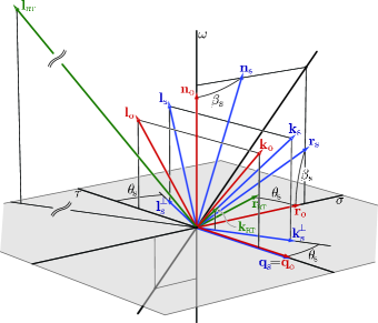
Figure 5: A spacetime diagram ($\varphi$ direction is suppressed) that depicts relations between the reference tetrad ${{{\boldsymbol{\mathbf{n}}}}_{\mathrm{o}},\,{{\boldsymbol{\mathbf{q}}}}_{\mathrm{o}},\,{{\boldsymbol{\mathbf{r}}}}_{\mathrm{o}},\,{{\boldsymbol{\mathbf{s}}}}_{\mathrm{o}}}$ (or ${{{\boldsymbol{\mathbf{k}}}}_{\mathrm{o}},\,{{\boldsymbol{\mathbf{l}}}}_{\mathrm{o}},\,{{\boldsymbol{\mathbf{m}}}}_{\mathrm{o}},\,{\bar{{\boldsymbol{\mathbf{m}}}}}_{\mathrm{o}}}$), the algebraically special tetrad ${{{\boldsymbol{\mathbf{n}}}}_{\mathrm{s}},\,{{\boldsymbol{\mathbf{q}}}}_{\mathrm{s}},\,{{\boldsymbol{\mathbf{r}}}}_{\mathrm{s}},\,{{\boldsymbol{\mathbf{s}}}}_{\mathrm{s}}}$ (or ${{{\boldsymbol{\mathbf{k}}}}_{\mathrm{s}},\,{{\boldsymbol{\mathbf{l}}}}_{\mathrm{s}},\,{{\boldsymbol{\mathbf{m}}}}_{\mathrm{s}},\,{\bar{{\boldsymbol{\mathbf{m}}}}}_{\mathrm{s}}}$), and the Robinson-Trautman tetrad ${{{\boldsymbol{\mathbf{k}}}}_{\scriptscriptstyle\mathrm{RT}},\,{{\boldsymbol{\mathbf{l}}}}_{\scriptscriptstyle\mathrm{RT}},\,{{\boldsymbol{\mathbf{m}}}}_{\scriptscriptstyle\mathrm{RT}},\,{\bar{{\boldsymbol{\mathbf{m}}}}}_{\scriptscriptstyle\mathrm{RT}}}$. The reference tetrad is naturally adapted to the infinity (${{\boldsymbol{\mathbf{n}}}}_{\mathrm{o}}$ is normal to ${\mathcal{I}}^{+}$) and the Killing vectors (${{\boldsymbol{\mathbf{q}}}}_{\mathrm{o}}$ and ${{\boldsymbol{\mathbf{s}}}}_{\mathrm{o}}$ are tangent to them), while the algebraically special tetrad is adapted to both double principal null directions ${{\boldsymbol{\mathbf{k}}}}_{\mathrm{s}}$ and ${{\boldsymbol{\mathbf{l}}}}_{\mathrm{s}}$. These two are related by a boost in the ${{{\boldsymbol{\mathbf{n}}}}_{\mathrm{o}}{\text{-}}{{\boldsymbol{\mathbf{r}}}}_{\mathrm{o}}}$ plane, with the boost parameter $\beta_{\mathrm{s}}$ given by Eq. (37). The vectors ${{\boldsymbol{\mathbf{q}}}}_{\mathrm{o}}$ and ${{\boldsymbol{\mathbf{q}}}}_{\mathrm{s}}$ are identical, similarly ${{{\boldsymbol{\mathbf{s}}}}_{\mathrm{o}}={{\boldsymbol{\mathbf{s}}}}_{\mathrm{s}}}$. Orthogonal projections ${{\boldsymbol{\mathbf{k}}}}_{\mathrm{s}}^{\perp}$, ${{\boldsymbol{\mathbf{l}}}}_{\mathrm{s}}^{\perp}$ of the principal null directions onto ${\omega=\text{constant}}$ hyperplane (shaded) define the angle $\theta_{\mathrm{s}}$ (Eq. (40)) that, similarly to $\beta_{\mathrm{s}}$, characterizes the relation between the reference and the special tetrads. The vector ${{\boldsymbol{\mathbf{k}}}}_{\scriptscriptstyle\mathrm{RT}}$ of the Robinson-Trautman tetrad points into the principal null direction ${{\boldsymbol{\mathbf{k}}}}_{\mathrm{s}}$ with the coefficient of proportionality approaching zero on ${\mathcal{I}}^{+}$, cf. Eq. (58). The other null direction ${{\boldsymbol{\mathbf{l}}}}_{\scriptscriptstyle\mathrm{RT}}$ belongs to the ${{{\boldsymbol{\mathbf{n}}}}_{\mathrm{o}}{\text{-}}{{\boldsymbol{\mathbf{k}}}}_{\mathrm{s}}}$ plane and it becomes “infinitely long” on ${\mathcal{I}}^{+}$.

We obtain even a better visualization if we perform a projection of the principal null directions ${{{\boldsymbol{\mathbf{k}}}}_{\mathrm{s}},\,{{\boldsymbol{\mathbf{l}}}}_{\mathrm{s}}}$ to a 3-dimensional hyperplane orthogonal to the timelike vector ${{\boldsymbol{\mathbf{n}}}}_{\mathrm{o}}$. We thus obtain “spatial” directions ${{{\boldsymbol{\mathbf{k}}}}_{\mathrm{s}}^{\perp},\,{{\boldsymbol{\mathbf{l}}}}_{\mathrm{s}}^{\perp}}$,

$${{\boldsymbol{\mathbf{k}}}}_{\mathrm{s}}^{\perp}={{\boldsymbol{\mathbf{k}}}}_{\mathrm{s}}+({{\boldsymbol{\mathbf{k}}}}_{\mathrm{s}}\mathbin{\boldsymbol{\cdot}}{{\boldsymbol{\mathbf{n}}}}_{\mathrm{o}})\,{{\boldsymbol{\mathbf{n}}}}_{\mathrm{o}}{\mbox{\;,\quad}}\text{etc.}{\mbox{\;,}}$$ (38)

of the null vectors ${{{\boldsymbol{\mathbf{k}}}}_{\mathrm{s}},\,{{\boldsymbol{\mathbf{l}}}}_{\mathrm{s}}}$ which lie in the ${{{\boldsymbol{\mathbf{q}}}}_{\mathrm{o}}{\text{-}}{{\boldsymbol{\mathbf{r}}}}_{\mathrm{o}}}$ plane, symmetrically with respect to the vector ${{\boldsymbol{\mathbf{r}}}}_{\mathrm{o}}$ (see Fig. 5). If we denote by $\theta_{\mathrm{s}}$ the angle between ${{\boldsymbol{\mathbf{q}}}}_{\mathrm{o}}$ and ${{\boldsymbol{\mathbf{k}}}}_{\mathrm{s}}^{\perp}$, we can write ${{{\boldsymbol{\mathbf{k}}}}_{\mathrm{s}}^{\perp}\propto\sin\theta_{\mathrm{s}}\,{{\boldsymbol{\mathbf{r}}}}_{\mathrm{o}}+\cos\theta_{\mathrm{s}}\,{{\boldsymbol{\mathbf{q}}}}_{\mathrm{o}}}$, and taking into account the normalization (25) we obtain

$$\begin{gathered}{{\boldsymbol{\mathbf{k}}}}_{\mathrm{s}}=\frac{1}{\sqrt{2}\cos\theta_{\mathrm{s}}}\,\bigl{(}{{\boldsymbol{\mathbf{n}}}}_{\mathrm{o}}+\sin\theta_{\mathrm{s}}\;{{\boldsymbol{\mathbf{r}}}}_{\mathrm{o}}+\cos\theta_{\mathrm{s}}\;{{\boldsymbol{\mathbf{q}}}}_{\mathrm{o}}\bigr{)}{\mbox{\;,}}\\ {{\boldsymbol{\mathbf{l}}}}_{\mathrm{s}}=\frac{1}{\sqrt{2}\cos\theta_{\mathrm{s}}}\,\bigl{(}{{\boldsymbol{\mathbf{n}}}}_{\mathrm{o}}+\sin\theta_{\mathrm{s}}\;{{\boldsymbol{\mathbf{r}}}}_{\mathrm{o}}-\cos\theta_{\mathrm{s}}\;{{\boldsymbol{\mathbf{q}}}}_{\mathrm{o}}\bigr{)}{\mbox{\;,}}\end{gathered}$$ (39)

cf.  also Eq. (177). Comparing this with relations (36) and using Eq. (23), we find that the angle $\theta_{\mathrm{s}}$ is given in terms of the metric functions ${{\mathcal{F}},\,{\mathcal{G}},\,{\mathcal{E}}}$ as

$$\sin\theta_{\mathrm{s}}=\sqrt{\frac{{\mathcal{G}}}{-{\mathcal{F}}}}\,\tanh\alpha{\mbox{\;,\quad}}\cos\theta_{\mathrm{s}}=\Bigl{(}\sqrt{\frac{{\mathcal{F}}}{{\mathcal{E}}}}\,\cosh\alpha\Bigr{)}^{-1}{\mbox{\;,}}$$ (40)

i.e., ${\tanh\beta_{\mathrm{s}}=\sin\theta_{\mathrm{s}}}$.

We will be interested mainly in the tetrads at the conformal infinity ${\mathcal{I}}^{+}$, i.e., for ${\omega=0}$, where ${\upsilon=\xi\tanh\alpha}$ and ${{\mathcal{E}}=-1}$, see Eqs. (18), (149). From the definitions (37), (40) and using Eqs. (135), (136) we find that the boost parameter $\beta_{\mathrm{s}}$ and the angle $\theta_{\mathrm{s}}$ (which both characterize directions “from the sources”) may on the ${\mathcal{I}}^{+}$ have values in the ranges

$$\beta_{\mathrm{s}}\in[0,\alpha]{\mbox{\;,\quad}}\sin\theta_{\mathrm{s}}\in[0,\tanh\alpha]{\mbox{\;.}}$$ (41)

The zero values occur on the axis of $\varphi$ symmetry (points “between” the moving black holes; ${\xi=\xi_{1},\xi_{2}}$), the maximal values occur on the “equator” — the $\varphi$ circle of maximal circumference (${\xi=0}$, ${\upsilon=0}$).

Transformation formulas (177) allow us to find components of the Weyl tensor and tensor of electromagnetic field in the reference null tetrad ${{{\boldsymbol{\mathbf{k}}}}_{\mathrm{o}},\,{{\boldsymbol{\mathbf{l}}}}_{\mathrm{o}},\,{{\boldsymbol{\mathbf{m}}}}_{\mathrm{o}},\,{\bar{{\boldsymbol{\mathbf{m}}}}}_{\mathrm{o}}}$, namely,

$$\begin{gathered}\Psi^{{\mathrm{o}}}_{2}={\textstyle{\frac{1}{2}}}\,\Psi^{{\mathrm{s}}}_{2}\,\bigl{(}3\cos^{-2}\theta_{\mathrm{s}}-1\bigr{)}{\mbox{\;,}}\\ \Psi^{{\mathrm{o}}}_{1}=\Psi^{{\mathrm{o}}}_{3}=-{\textstyle{\frac{3}{2}}}\,\Psi^{{\mathrm{s}}}_{2}\;{\sin\theta_{\mathrm{s}}}\;{\cos^{-2}\theta_{\mathrm{s}}}{\mbox{\;,}}\\ \Psi^{{\mathrm{o}}}_{0}=\Psi^{{\mathrm{o}}}_{4}={\textstyle{\frac{3}{2}}}\,\Psi^{{\mathrm{s}}}_{2}\;{\sin^{2}\theta_{\mathrm{s}}}\;{\cos^{-2}\theta_{\mathrm{s}}}{\mbox{\;,}}\end{gathered}$$ (45)

$$\Phi^{{\mathrm{o}}}_{0}=\Phi^{{\mathrm{o}}}_{2}=-\tan\theta_{\mathrm{s}}\,\Phi^{{\mathrm{s}}}_{1}{\mbox{\;,\quad}}\Phi^{{\mathrm{o}}}_{1}=\cos^{-1}\theta_{\mathrm{s}}\,\Phi^{{\mathrm{s}}}_{1}{\mbox{\;,}}$$ (46)

or, more explicitly (using Eqs. (32), (34), and (40))

$$\begin{gathered}\Psi^{{\mathrm{o}}}_{2}=\frac{{\mathcal{F}}^{\prime\prime}+{\mathcal{G}}^{\prime\prime}}{8\,{\mathcal{E}}\,r^{2}}\,\frac{1}{3}\bigl{(}2{\mathcal{F}}\cosh^{2}\alpha-{\mathcal{G}}\sinh^{2}\alpha\bigr{)}{\mbox{\;,}}\\ \Psi^{{\mathrm{o}}}_{1}=\Psi^{{\mathrm{o}}}_{3}=\frac{{\mathcal{F}}^{\prime\prime}+{\mathcal{G}}^{\prime\prime}}{8\,{\mathcal{E}}\,r^{2}}\,\sqrt{-{\mathcal{F}}{\mathcal{G}}}\,\cosh\alpha\,\sinh\alpha{\mbox{\;,}}\\ \Psi^{{\mathrm{o}}}_{0}=\Psi^{{\mathrm{o}}}_{4}=-\frac{{\mathcal{F}}^{\prime\prime}+{\mathcal{G}}^{\prime\prime}}{8\,{\mathcal{E}}\,r^{2}}\,{\mathcal{G}}\,\sinh^{2}\alpha{\mbox{\;,}}\end{gathered}$$ (50)

$$\begin{gathered}\Phi^{{\mathrm{o}}}_{1}=-\frac{e}{2\,r^{2}}\,\sqrt{\frac{{\mathcal{F}}}{{\mathcal{E}}}}\,\cosh\alpha{\mbox{\;,}}\\ \Phi^{{\mathrm{o}}}_{0}=\Phi^{{\mathrm{o}}}_{2}=\frac{e}{2\,r^{2}}\,\sqrt{\frac{{\mathcal{G}}}{-{\mathcal{E}}}}\,\sinh\alpha{\mbox{\;.}}\end{gathered}$$ (53)

As we have already mentioned, the tetrad ${{{\boldsymbol{\mathbf{n}}}}_{\mathrm{o}},\,{{\boldsymbol{\mathbf{q}}}}_{\mathrm{o}},\,{{\boldsymbol{\mathbf{r}}}}_{\mathrm{o}},\,{{\boldsymbol{\mathbf{s}}}}_{\mathrm{o}}}$ serves as the reference tetrad with respect to which we characterize an arbitrarily rotated tetrad ${{{\boldsymbol{\mathbf{n}}}}_{\mathrm{r}},\,{{\boldsymbol{\mathbf{q}}}}_{\mathrm{r}},\,{{\boldsymbol{\mathbf{r}}}}_{\mathrm{r}},\,{{\boldsymbol{\mathbf{s}}}}_{\mathrm{r}}}$. The tetrad ${{{\boldsymbol{\mathbf{n}}}}_{\mathrm{r}},\,{{\boldsymbol{\mathbf{q}}}}_{\mathrm{r}},\,{{\boldsymbol{\mathbf{r}}}}_{\mathrm{r}},\,{{\boldsymbol{\mathbf{s}}}}_{\mathrm{r}}}$ is obtained from the reference tetrad by a spatial rotation given by angles ${\theta,\,\phi}$,

$${{\boldsymbol{\mathbf{n}}}}_{\mathrm{r}} ={{\boldsymbol{\mathbf{n}}}}_{\mathrm{o}}{\mbox{\;,}}$$ (54)

$${{\boldsymbol{\mathbf{q}}}}_{\mathrm{r}} ={\mspace{14.5mu}}\cos\theta\;{{\boldsymbol{\mathbf{q}}}}_{\mathrm{o}}+\sin\theta\cos\phi\;{{\boldsymbol{\mathbf{r}}}}_{\mathrm{o}}+\sin\theta\sin\phi\;{{\boldsymbol{\mathbf{s}}}}_{\mathrm{o}}{\mbox{\;,}}$$

$${{\boldsymbol{\mathbf{r}}}}_{\mathrm{r}} =-\sin\theta\;{{\boldsymbol{\mathbf{q}}}}_{\mathrm{o}}+\cos\theta\cos\phi\;{{\boldsymbol{\mathbf{r}}}}_{\mathrm{o}}+\cos\theta\sin\phi\;{{\boldsymbol{\mathbf{s}}}}_{\mathrm{o}}{\mbox{\;,}}$$

$${{\boldsymbol{\mathbf{s}}}}_{\mathrm{r}} =\mspace{120.0mu}-\sin\phi\;{{\boldsymbol{\mathbf{r}}}}_{\mathrm{o}}+\qquad\,\cos\phi\;{{\boldsymbol{\mathbf{s}}}}_{\mathrm{o}}{\mbox{\;.}}$$

Let us note that the angles ${\theta,\,\phi}$, understood as standard spherical coordinates spanned on the axes ${{{\boldsymbol{\mathbf{q}}}}_{\mathrm{o}},\,{{\boldsymbol{\mathbf{r}}}}_{\mathrm{o}},\,{{\boldsymbol{\mathbf{s}}}}_{\mathrm{o}}}$, describe exactly the spatial direction ${{{\boldsymbol{\mathbf{k}}}}_{\mathrm{r}}^{\perp}=\frac{1}{\sqrt{2}}{{\boldsymbol{\mathbf{q}}}}_{\mathrm{r}}}$ of the null vector ${{\boldsymbol{\mathbf{k}}}}_{\mathrm{r}}$, where the spatial direction means projection orthogonal to the vector ${{\boldsymbol{\mathbf{n}}}}_{\mathrm{o}}$. The relation between null tetrads following from Eq. (54) can be found in Eq. (179). This transformation is obtained as a consecutive composition of null rotation with fixed ${{\boldsymbol{\mathbf{k}}}}$ (Eq. (182)), null rotation with fixed ${{\boldsymbol{\mathbf{l}}}}$ (Eq. (185)), and of special boost and spatial rotation (188) with parameters

$$L =-\tan\frac{\theta}{2}\,\exp(-i\phi){\mbox{\;,}}$$ (55)

$$K =\sin\frac{\theta}{2}\,\cos\frac{\theta}{2}\,\exp(-i\phi){\mbox{\;,}}$$

$$B =\cos^{-2}\frac{\theta}{2}{\mbox{\;,\quad}}\Phi=\phi{\mbox{\;.}}$$

Finally, we also introduce the Robinson-Trautman tetrad ${{{\boldsymbol{\mathbf{k}}}}_{\scriptscriptstyle\mathrm{RT}},\,{{\boldsymbol{\mathbf{l}}}}_{\scriptscriptstyle\mathrm{RT}},\,{{\boldsymbol{\mathbf{m}}}}_{\scriptscriptstyle\mathrm{RT}},\,{\bar{{\boldsymbol{\mathbf{m}}}}}_{\scriptscriptstyle\mathrm{RT}}}$ (see, e.g., Kramer et al. (1980)) naturally connected with the Robinson-Trautman coordinates ${\zeta,\,\bar{\zeta},\,u,\,r}$ (cf.  Eqs. (9) and (150), (153))

$${{\boldsymbol{\mathbf{k}}}}_{\scriptscriptstyle\mathrm{RT}} ={{\boldsymbol{\mathbf{\partial}}}_{r}}{\mbox{\;,}}$$ (56)

$${{\boldsymbol{\mathbf{l}}}}_{\scriptscriptstyle\mathrm{RT}} =-\textstyle{\frac{1}{2}}H\,{{\boldsymbol{\mathbf{\partial}}}_{r}}+{{\boldsymbol{\mathbf{\partial}}}_{u}}\mspace{-12.0mu} =-\frac{r^{2}\,{\mathcal{E}}}{2\,a_{\scriptscriptstyle\Lambda}^{2}}\,{{\boldsymbol{\mathbf{\partial}}}_{r}}+{{\boldsymbol{\mathbf{\partial}}}_{u}}{\mbox{\;,}}$$

$${{\boldsymbol{\mathbf{m}}}}_{\scriptscriptstyle\mathrm{RT}} =\frac{P}{r}\,{{\boldsymbol{\mathbf{\partial}}}_{\bar{\zeta}}} =\frac{1}{\sqrt{\mathcal{G}}\,r}\,{{\boldsymbol{\mathbf{\partial}}}_{\bar{\zeta}}}{\mbox{\;,}}$$

$${\bar{{\boldsymbol{\mathbf{m}}}}}_{\scriptscriptstyle\mathrm{RT}} =\frac{P}{r}\,{{\boldsymbol{\mathbf{\partial}}}_{\zeta}} =\frac{1}{\sqrt{\mathcal{G}}\,r}\,{{\boldsymbol{\mathbf{\partial}}}_{\zeta}}{\mbox{\;.}}$$

Here we have written down equivalent expressions using both metric functions $H$, $P$ commonly used in the Robinson-Trautman framework, and the metric functions ${\mathcal{G}}$, ${\mathcal{E}}$ of the $C$-metric (cf.  Eqs. (14), (15)). The vector ${{\boldsymbol{\mathbf{k}}}}_{\scriptscriptstyle\mathrm{RT}}$ of this tetrad is oriented along the principal null direction ${{\boldsymbol{\mathbf{k}}}}_{\mathrm{s}}$, and it will be demonstrated in Section VII that this tetrad is parallelly transported along the geodesics tangent to principal null directions.

The tetrad (56) is simply related to the particularly rotated tetrad ${{{\boldsymbol{\mathbf{k}}}}_{\mathrm{r}},\,{{\boldsymbol{\mathbf{l}}}}_{\mathrm{r}},\,{{\boldsymbol{\mathbf{m}}}}_{\mathrm{r}},\,{\bar{{\boldsymbol{\mathbf{m}}}}}_{\mathrm{r}}}$ (Eq. (179)) with ${\theta=\theta_{\mathrm{s}}}$, ${\phi=0}$, ${\theta_{\mathrm{s}}}$ given by Eq. (40):

$$\begin{gathered}{{\boldsymbol{\mathbf{k}}}}_{\scriptscriptstyle\mathrm{RT}}=\exp(\beta_{\scriptscriptstyle\mathrm{RT}}){{\boldsymbol{\mathbf{k}}}}_{\mathrm{r}}{\mbox{\;,\quad}}{{\boldsymbol{\mathbf{l}}}}_{\scriptscriptstyle\mathrm{RT}}=\exp(-\beta_{\scriptscriptstyle\mathrm{RT}}){{\boldsymbol{\mathbf{l}}}}_{\mathrm{r}}{\mbox{\;,}}\\ {{\boldsymbol{\mathbf{m}}}}_{\scriptscriptstyle\mathrm{RT}}={{\boldsymbol{\mathbf{m}}}}_{\mathrm{r}}{\mbox{\;,\quad}}{\bar{{\boldsymbol{\mathbf{m}}}}}_{\scriptscriptstyle\mathrm{RT}}={\bar{{\boldsymbol{\mathbf{m}}}}}_{\mathrm{r}}{\mbox{\;,}}\end{gathered}$$ (57)

i.e., the Robinson-Trautman tetrad can be obtained from the reference tetrad ${{{\boldsymbol{\mathbf{k}}}}_{\mathrm{o}},\,{{\boldsymbol{\mathbf{l}}}}_{\mathrm{o}},\,{{\boldsymbol{\mathbf{m}}}}_{\mathrm{o}},\,{\bar{{\boldsymbol{\mathbf{m}}}}}_{\mathrm{o}}}$ by the spatial rotation (179) with ${\theta=\theta_{\mathrm{s}}}$, ${\phi=0}$, followed by the boost (188) with the parameter

$$B=\exp\beta_{\scriptscriptstyle\mathrm{RT}}=-\frac{\sqrt{2}\,\omega}{\sqrt{-{\mathcal{E}}}}=\sqrt{-\frac{2}{H}}{\mbox{\;.}}$$ (58)

We also give the relation between the Robinson-Trautman and the algebraically special tetrad. Because the vectors ${{\boldsymbol{\mathbf{k}}}}_{\scriptscriptstyle\mathrm{RT}}$ and ${{\boldsymbol{\mathbf{k}}}}_{\mathrm{s}}$ are proportional, the Robinson-Trautman tetrad is obtained from the special tetrad by the null rotation (182) followed by the boost (188) with parameters

$$L =-\sin\theta_{\mathrm{s}}\mspace{46.0mu}=-\sqrt{\frac{{\mathcal{G}}}{-{\mathcal{F}}}}\,\tanh\alpha{\mbox{\;,}}$$ (59)

$$B =\exp\beta_{\scriptscriptstyle\mathrm{RT}}\cos\theta_{\mathrm{s}}=\frac{\sqrt{2}\,a_{\scriptscriptstyle\Lambda}}{r\sqrt{-{\mathcal{F}}}\,\cosh\alpha}{\mbox{\;.}}$$

The explicit relation of both tetrads can be found in Eqs. (177) and (178).

Using the transformations (183), (190) and (184), (191) with these parameters $L$, $B$, we find that the only nonvanishing components of the gravitational and electromagnetic fields in the Robinson-Trautman tetrad are

$$\begin{gathered}\Psi^{{\scriptscriptstyle\mathrm{RT}}}_{2}=\Psi^{{\mathrm{s}}}_{2}=-\Bigl{(}m-2\,e^{2}A\,\xi-\frac{e^{2}}{r}\Bigr{)}\,\frac{1}{r^{3}}{\mbox{\;,}}\\ \Psi^{{\scriptscriptstyle\mathrm{RT}}}_{3}=-\frac{3}{\sqrt{2}}\,\frac{A\,r}{P}\,\Psi^{{\mathrm{s}}}_{2}{\mbox{\;,\quad}}\Psi^{{\scriptscriptstyle\mathrm{RT}}}_{4}=3\,\frac{A^{2}\,r^{2}}{P^{2}}\,\Psi^{{\mathrm{s}}}_{2}{\mbox{\;,}}\end{gathered}$$ (62)

$$\Phi^{{\scriptscriptstyle\mathrm{RT}}}_{1}=\Phi^{{\mathrm{s}}}_{1}=-\frac{e}{2\,r^{2}}{\mbox{\;,\quad}}\Phi^{{\scriptscriptstyle\mathrm{RT}}}_{2}=-\sqrt{2}\,\frac{A\,r}{P}\,\Phi^{{\mathrm{s}}}_{1}{\mbox{\;,}}$$ (63)

with $\Psi^{{\mathrm{s}}}_{2}$ and $\Phi^{{\mathrm{s}}}_{1}$ also given by Eqs. (32) and (34), cf.  Kramer et al. (1980).

V Gravitational and electromagnetic fields near ${\mathcal{I}}^{+}$

Now we are prepared to discuss radiative properties of the $C$-metric fields near the de Sitter-like infinity ${\mathcal{I}}^{+}$. As we have already explained in Section I, by the radiative field we understand a field with a dominant component having the $1/\eta$ fall-off, calculated in a tetrad parallelly transported along a null geodesic $z(\eta)$. We will in particular concentrate on investigation of a directional dependence of the gravitational and electromagnetic radiation.

To study the dependence of the fields on the directions along which the spacelike infinity ${\mathcal{I}}^{+}$ is approached, it is crucial to find a parallelly transported tetrad along all null geodesics. However, it is difficult to find a general geodesic and the corresponding tetrad in an explicit form, except for the case of very special geodesics along the privileged principal null directions, which will be discussed in Section VII. Fortunately, it is not, in fact, necessary to find an explicit form of the geodesics and tetrads because we are interested only in the dominant terms of the fields close to ${\mathcal{I}}^{+}$. It is fully sufficient to study only their asymptotic forms.

Near infinity ${\mathcal{I}}^{+}$, null geodesics $z(\eta)$ can be expanded in the inverse powers of the affine parameter ${\eta\to\infty}$. In particular, in coordinates ${\tau,\,\omega,\,\sigma,\,\varphi}$ introduced in Eq. (11), the null geodesics $z(\eta)$ can be expanded as

$$\omega(\eta) \approx\mspace{40.0mu}\omega_{*}\,\frac{a_{\scriptscriptstyle\Lambda}}{\eta}+\dots\mbox{\;,}$$ (64)

$$\tau(\eta) \approx\tau_{\scriptscriptstyle{\boldsymbol{+}}}+\tau_{*}\,\frac{a_{\scriptscriptstyle\Lambda}}{\eta}+\dots\mbox{\;,}$$

$$\sigma(\eta) \approx\sigma_{\scriptscriptstyle{\boldsymbol{+}}}+\sigma_{*}\,\frac{a_{\scriptscriptstyle\Lambda}}{\eta}+\dots\mbox{\;,}$$

$$\varphi(\eta) \approx\varphi_{\scriptscriptstyle{\boldsymbol{+}}}+\varphi_{*}\,\frac{a_{\scriptscriptstyle\Lambda}}{\eta}+\dots\mbox{\;,}$$

where the affine parameter $\eta$ has the dimension of length. There is no absolute term in the expansion of the coordinate $\omega$ because ${\omega=0}$ at ${\mathcal{I}}^{+}$. The constant parameters ${\tau_{\scriptscriptstyle{\boldsymbol{+}}},\,\sigma_{\scriptscriptstyle{\boldsymbol{+}}},\,\varphi_{\scriptscriptstyle{\boldsymbol{+}}}}$ (and the corresponding values $\upsilon_{\scriptscriptstyle{\boldsymbol{+}}}$ and $\xi_{\scriptscriptstyle{\boldsymbol{+}}}$ given by Eq. (11)) label the point $N_{\scriptscriptstyle{\boldsymbol{+}}}$ at ${\mathcal{I}}^{+}$ which is approached by the geodesic $z(\eta)$. The parameters ${\tau_{*},\,\sigma_{*},\,\varphi_{*}}$ characterize the direction along which this point $N_{\scriptscriptstyle{\boldsymbol{+}}}$ is approached. The remaining coefficient $\omega_{*}$ can be determined from the normalization of the tangent vector which must be null. The tangent vector has the form

$$\begin{split}\frac{Dz}{d\eta}\approx-\frac{a_{\scriptscriptstyle\Lambda}}{\eta^{2}}\,\bigl{(}\omega_{*}\,{{\boldsymbol{\mathbf{\partial}}}_{\omega}}+\tau_{*}\,{{\boldsymbol{\mathbf{\partial}}}_{\tau}}+\sigma_{*}\,{{\boldsymbol{\mathbf{\partial}}}_{\sigma}}+\varphi_{*}\,{{\boldsymbol{\mathbf{\partial}}}_{\varphi}}\bigr{)}{\mbox{\;.}}\end{split}$$ (65)

The asymptotic form of the metric (12) along the null geodesic is

$${\boldsymbol{g}}\approx\frac{\eta^{2}}{\omega_{*}^{2}}\,\bigl{(}-\mathbf{d}\omega^{2}-{\mathcal{F}}_{\scriptscriptstyle{\boldsymbol{+}}}\,\mathbf{d}\tau^{2}-{\mathcal{F}}_{\scriptscriptstyle{\boldsymbol{+}}}{\mathcal{G}}_{\scriptscriptstyle{\boldsymbol{+}}}\,\mathbf{d}\sigma^{2}+{\mathcal{G}}_{\scriptscriptstyle{\boldsymbol{+}}}\mathbf{d}\varphi^{2}\bigr{)}{\mbox{\;,}}$$ (66)

where ${\mathcal{F}}_{\scriptscriptstyle{\boldsymbol{+}}}$ and ${\mathcal{G}}_{\scriptscriptstyle{\boldsymbol{+}}}$ are the functions ${\mathcal{F}}$ and ${\mathcal{G}}$ evaluated at the point $N_{\scriptscriptstyle{\boldsymbol{+}}}$ at infinity ${\mathcal{I}}^{+}$, and we used ${{\mathcal{E}}_{\scriptscriptstyle{\boldsymbol{+}}}=-1}$. Therefore, the condition that the tangent vector is a null vector implies

$$\omega_{*}^{2}=-{\mathcal{F}}_{\scriptscriptstyle{\boldsymbol{+}}}\tau_{*}^{2}-{\mathcal{F}}_{\scriptscriptstyle{\boldsymbol{+}}}{\mathcal{G}}_{\scriptscriptstyle{\boldsymbol{+}}}\sigma_{*}^{2}+{\mathcal{G}}_{\scriptscriptstyle{\boldsymbol{+}}}\varphi_{*}^{2}{\mbox{\;.}}$$ (67)

Notice that ${\omega_{*}<0}$ since ${\omega<0}$, and

$$r(\eta)\approx\gamma\,\eta+\dots\mbox{\;,\quad}\text{where}\quad\gamma=-\frac{1}{\omega_{*}}{\mbox{\;,}}$$ (68)

which follows from Eq. (16).

We wish to compare geodesics approaching the given point $N_{\scriptscriptstyle{\boldsymbol{+}}}$ along different directions. We thus need to ensure “the same” universal choice of the affine parameter $\eta$ for all geodesics. It is natural to require that the energy (or, equivalently, the frequency) of the ray represented by the null geodesic

$$E_{\mathrm{o}}=-{{\boldsymbol{\mathbf{p}}}}\mathbin{\boldsymbol{\cdot}}{{\boldsymbol{\mathbf{n}}}}_{\mathrm{o}}=-a_{\scriptscriptstyle\Lambda}\,\frac{Dz}{d\eta}\mathbin{\boldsymbol{\cdot}}{{\boldsymbol{\mathbf{n}}}}_{\mathrm{o}}$$ (69)

(see note nt:PhysAffinePar ), is the same independently of the direction of the geodesic, i.e., that the component of the tangent vector to the normal direction ${{\boldsymbol{\mathbf{n}}}}_{\mathrm{o}}$ is fixed. From Eqs. (69), (65), and (35) it immediately follows that

$$E_{\mathrm{o}}\approx\frac{a_{\scriptscriptstyle\Lambda}^{2}}{\eta}=\gamma\,\frac{a_{\scriptscriptstyle\Lambda}^{2}}{r}{\mbox{\;.}}$$ (70)

The value of the energy $E_{\mathrm{o}}$ with respect to any asymptotic observer characterized by the 4-velocity ${{\boldsymbol{\mathbf{n}}}}_{\mathrm{o}}$ thus obviously approaches zero as ${\eta\to\infty}$. This behavior is caused by the de Sitter-like character of ${\mathcal{I}}^{+}$. Therefore, we have to compare the values of $E_{\mathrm{o}}$ at the same “proximity” to ${\mathcal{I}}^{+}$, i.e., at some fixed large but finite value of the coordinate $r$ (note nt:Proximity ). We conclude from Eq. (70) that fixing the energy at a given prescribed value of $r$ is equivalent to fixing the value of the constant parameter $\gamma$ independently of a direction of the geodesic. Let us note that this approach is fully equivalent to fixing a finite value of conformal energy, i.e., of the energy defined with respect to a vector normal to ${\mathcal{I}}^{+}$ normalized using a conformal metric ${\tilde{{\boldsymbol{g}}}=\omega^{2}{\boldsymbol{g}}}$.

Next, it is necessary to find an interpretation tetrad ${{{\boldsymbol{\mathbf{k}}}}_{\mathrm{i}},\,{{\boldsymbol{\mathbf{l}}}}_{\mathrm{i}},\,{{\boldsymbol{\mathbf{m}}}}_{\mathrm{i}},\,{\bar{{\boldsymbol{\mathbf{m}}}}}_{\mathrm{i}}}$ which is parallelly transported along the geodesic $z(\eta)$. However, using only an asymptotic expansion of the tetrad at infinity ${\mathcal{I}}^{+}$, we cannot determine unique initial conditions which define this tetrad somewhere in a finite region of the spacetime. But without specifying these initial conditions, the parallelly transported tetrad at ${\mathcal{I}}^{+}$ is given only up to an arbitrary (finite) Lorentz transformation. It thus seems that we are losing all information because of this nonuniqueness. However, it is not so. It will be demonstrated that the crucial information about the behavior of the fields at infinity ${\mathcal{I}}^{+}$ is hidden in an “infinite” Lorentz transformation corresponding to the parallel transport from a finite region of the spacetime up to the infinity. It will thus be sufficient to find only the leading term of this transformation.

To be more specific, we naturally choose the vector ${{\boldsymbol{\mathbf{k}}}}_{\mathrm{i}}$ of the parallelly transported interpretation null tetrad to be proportional to the (parallelly transported) tangent vector of the geodesic. This ensures that ${{\boldsymbol{\mathbf{k}}}}_{\mathrm{i}}$ is finite in finite regions of spacetime (see note nt:ArbFinCnd ). However, we still have a freedom in the normalization of ${{\boldsymbol{\mathbf{k}}}}_{\mathrm{i}}$ which can be multiplied by an arbitrary finite factor, constant along the geodesic. Similarly to the choice of the “universal” affine parameter for different geodesics, we have to choose the parallelly transported tetrads in some suitable “comparable” way for various geodesics approaching the same point $N_{\scriptscriptstyle{\boldsymbol{+}}}$ at infinity from different directions. Not having an explicit form of the geodesics (except for those special ones discussed in Section VII), we have to eliminate the dependence on initial conditions by fixing final conditions for the tetrad at infinity ${\mathcal{I}}^{+}$. Namely, we will require that the normalization of the vector ${{\boldsymbol{\mathbf{k}}}}_{\mathrm{i}}$ is specified independently of the direction of the geodesics. This is achieved, for example, by the condition

$${{\boldsymbol{\mathbf{k}}}}_{\mathrm{i}}\cdot\mathbf{d}r=1{\mbox{\;.}}$$ (71)

Thanks to Eq. (68) we thus have

$${{\boldsymbol{\mathbf{k}}}}_{\mathrm{i}}=\frac{1}{\gamma}\,\frac{Dz}{d\eta}{\mbox{\;.}}$$ (72)

Concerning vectors ${{{\boldsymbol{\mathbf{m}}}}_{\mathrm{i}},\,{\bar{{\boldsymbol{\mathbf{m}}}}}_{\mathrm{i}}}$ of the parallelly transported interpretation tetrad, there is a priori no “canonical” prescription how to choose these in a universal way for different geodesics. The only constraint is the correct normalization (25). Therefore, we have to find such physical quantities which are invariant under this freedom. It will be shown below (see Eq. (81) and discussion therein) that the magnitude of the leading term of the fields at ${\mathcal{I}}^{+}$ is, in fact, independent of the specific choice of the vectors ${{{\boldsymbol{\mathbf{m}}}}_{\mathrm{i}},\,{\bar{{\boldsymbol{\mathbf{m}}}}}_{\mathrm{i}}}$.

However, there is a natural possibility to fix the null vector ${{\boldsymbol{\mathbf{l}}}}_{\mathrm{i}}$ of the tetrad by the condition that the timelike unit vector ${{\boldsymbol{\mathbf{n}}}}_{\mathrm{o}}$, orthogonal to infinity ${\mathcal{I}}^{+}$, lies in the ${{{\boldsymbol{\mathbf{k}}}}_{\mathrm{i}}{\text{-}}{{\boldsymbol{\mathbf{l}}}}_{\mathrm{i}}}$ plane. In this case the parallelly transported tetrad can be obtained by a boost in the ${{{\boldsymbol{\mathbf{k}}}}_{\mathrm{i}}{\text{-}}{{\boldsymbol{\mathbf{l}}}}_{\mathrm{i}}}$ plane from the rotated tetrad ${{{\boldsymbol{\mathbf{k}}}}_{\mathrm{r}},\,{{\boldsymbol{\mathbf{l}}}}_{\mathrm{r}},\,{{\boldsymbol{\mathbf{m}}}}_{\mathrm{r}},\,{\bar{{\boldsymbol{\mathbf{m}}}}}_{\mathrm{r}}}$ (see Eqs. (54) or (179)) with properly chosen angles ${\theta,\,\phi}$. Clearly, the vector ${{\boldsymbol{\mathbf{k}}}}_{\mathrm{r}}$ has to point exactly in the direction of the geodesic, or equivalently, the spatial vector ${{\boldsymbol{\mathbf{q}}}}_{\mathrm{r}}$ has to point in the spatial direction of the geodesic (here again by spatial vectors we mean those orthogonal to ${{{\boldsymbol{\mathbf{n}}}}_{\mathrm{o}}={{\boldsymbol{\mathbf{n}}}}_{\mathrm{r}}}$, i.e., tangent to ${\mathcal{I}}^{+}$). Using Eqs. (72), (65), and (35) we obtain

$${{\boldsymbol{\mathbf{k}}}}_{\mathrm{i}}\approx\frac{a_{\scriptscriptstyle\Lambda}}{\gamma\,\eta}\,\Bigl{(}{{\boldsymbol{\mathbf{n}}}}_{\mathrm{o}}-\frac{1}{\eta}\,\bigl{(}\tau_{*}\,{{\boldsymbol{\mathbf{\partial}}}_{\tau}}+\sigma_{*}\,{{\boldsymbol{\mathbf{\partial}}}_{\sigma}}+\varphi_{*}\,{{\boldsymbol{\mathbf{\partial}}}_{\varphi}}\bigr{)}\Bigr{)}{\mbox{\;.}}$$ (73)

The unit vector ${{\boldsymbol{\mathbf{q}}}}_{\mathrm{r}}$ in the spatial direction of the geodesic is thus

$${{\boldsymbol{\mathbf{q}}}}_{\mathrm{r}} \approx-\frac{1}{\eta}\,\Bigl{(}\tau_{*}\,{{\boldsymbol{\mathbf{\partial}}}_{\tau}}+\sigma_{*}\,{{\boldsymbol{\mathbf{\partial}}}_{\sigma}}+\varphi_{*}\,{{\boldsymbol{\mathbf{\partial}}}_{\varphi}}\Bigr{)}$$ (74)

$$=-\sqrt{-{\mathcal{F}}_{\scriptscriptstyle{\boldsymbol{+}}}}\,\frac{\tau_{*}}{\omega_{*}}\,{{\boldsymbol{\mathbf{q}}}}_{\mathrm{o}}+\sqrt{-{\mathcal{F}}_{\scriptscriptstyle{\boldsymbol{+}}}{\mathcal{G}}_{\scriptscriptstyle{\boldsymbol{+}}}}\,\frac{\sigma_{*}}{\omega_{*}}\,{{\boldsymbol{\mathbf{r}}}}_{\mathrm{o}}+\sqrt{{\mathcal{G}}_{\scriptscriptstyle{\boldsymbol{+}}}}\,\frac{\varphi_{*}}{\omega_{*}}\,{{\boldsymbol{\mathbf{s}}}}_{\mathrm{o}}{\mbox{\;.}}$$

The leading term of the expansion of the parallelly transported tetrad near the infinity then can be written as

$${{\boldsymbol{\mathbf{k}}}}_{\mathrm{i}} \approx\frac{\sqrt{2}\,a_{\scriptscriptstyle\Lambda}}{\gamma\,\eta}\,{{\boldsymbol{\mathbf{k}}}}_{\mathrm{r}}=\frac{a_{\scriptscriptstyle\Lambda}}{\gamma\,\eta}\,({{\boldsymbol{\mathbf{n}}}}_{\mathrm{o}}+{{\boldsymbol{\mathbf{q}}}}_{\mathrm{r}}){\mbox{\;,}} {{\boldsymbol{\mathbf{m}}}}_{\mathrm{i}} \approx{{\boldsymbol{\mathbf{m}}}}_{\mathrm{r}}{\mbox{\;,}}$$ (75)

$${{\boldsymbol{\mathbf{l}}}}_{\mathrm{i}} \approx\frac{\gamma\,\eta}{\sqrt{2}\,a_{\scriptscriptstyle\Lambda}}\;{{\boldsymbol{\mathbf{l}}}}_{\mathrm{r}}\;=\frac{\gamma\,\eta}{2a_{\scriptscriptstyle\Lambda}}\,({{\boldsymbol{\mathbf{n}}}}_{\mathrm{o}}-{{\boldsymbol{\mathbf{q}}}}_{\mathrm{r}}){\mbox{\;,}} {\bar{{\boldsymbol{\mathbf{m}}}}}_{\mathrm{i}} \approx{\bar{{\boldsymbol{\mathbf{m}}}}}_{\mathrm{r}}{\mbox{\;.}}$$

Here, we have made a particular choice of the vectors ${{{\boldsymbol{\mathbf{m}}}}_{\mathrm{i}},\,{\bar{{\boldsymbol{\mathbf{m}}}}}_{\mathrm{i}}}$. In general, ${{\boldsymbol{\mathbf{m}}}}_{\mathrm{i}}$ could differ from ${{\boldsymbol{\mathbf{m}}}}_{\mathrm{r}}$ by a phase factor (a rotation in the ${{{\boldsymbol{\mathbf{m}}}}_{\mathrm{i}}{\text{-}}{\bar{{\boldsymbol{\mathbf{m}}}}}_{\mathrm{i}}}$ plane) which, as we mentioned, cannot be fixed in a canonical way. Our choice ${{{\boldsymbol{\mathbf{m}}}}_{\mathrm{i}}\approx{{\boldsymbol{\mathbf{m}}}}_{\mathrm{r}}}$ is “natural” for the approach presented here. However, in the next section we will encounter another “suitable” choice of the vector ${{\boldsymbol{\mathbf{m}}}}_{\mathrm{i}}$.

Now we have to identify the angles ${\theta,\,\phi}$. Let us recall that these angles are just spherical coordinates of the spatial direction ${{{\boldsymbol{\mathbf{q}}}}_{\mathrm{r}}\propto{{\boldsymbol{\mathbf{k}}}}_{\mathrm{i}}^{\perp}}$ with respect to the reference frame ${{{\boldsymbol{\mathbf{q}}}}_{\mathrm{o}},\,{{\boldsymbol{\mathbf{r}}}}_{\mathrm{o}},\,{{\boldsymbol{\mathbf{s}}}}_{\mathrm{o}}}$. Comparing Eqs. (74) and (54) we find that the parameters ${\tau_{*},\,\sigma_{*},\,\varphi_{*}}$, characterizing the asymptotic spatial direction of the geodesic (64), fix the the angles ${\theta,\,\phi}$ as

$$\tau_{*} ={\mspace{14.5mu}}\frac{1}{\gamma\sqrt{-{\mathcal{F}}_{\scriptscriptstyle{\boldsymbol{+}}}}}\,\cos\theta{\mbox{\;,}}$$ (76)

$$\sigma_{*} =-\frac{1}{\gamma\sqrt{-{\mathcal{F}}_{\scriptscriptstyle{\boldsymbol{+}}}{\mathcal{G}}_{\scriptscriptstyle{\boldsymbol{+}}}}}\,\sin\theta\cos\phi{\mbox{\;,}}$$

$$\varphi_{*} =-\frac{1}{\gamma\sqrt{{\mathcal{G}}_{\scriptscriptstyle{\boldsymbol{+}}}}}\,\sin\theta\sin\phi{\mbox{\;.}}$$

In the following we will use these angles ${\theta,\,\phi}$ to parametrize the direction along which a null geodesic approaches the point $N_{\scriptscriptstyle{\boldsymbol{+}}}$ on ${\mathcal{I}}^{+}$.

Now we are ready to calculate the leading terms of the components $\Psi^{{\mathrm{i}}}_{n}$ of the Weyl tensor in the parallelly transported tetrad given above. First we find the components $\Psi^{{\mathrm{r}}}_{n}$ in the rotated tetrad ${{{\boldsymbol{\mathbf{k}}}}_{\mathrm{r}},\,{{\boldsymbol{\mathbf{l}}}}_{\mathrm{r}},\,{{\boldsymbol{\mathbf{m}}}}_{\mathrm{r}},\,{\bar{{\boldsymbol{\mathbf{m}}}}}_{\mathrm{r}}}$. These can easily be obtained from Eq. (50) using relations (183), (186), and (190) with the parameters (55). Notice that all these components are of the same order in $\eta$, namely, ${\sim\eta^{-3}}$ (cf.  also Eq. (80) below). To obtain the components $\Psi^{{\mathrm{i}}}_{n}$ in the parallelly transported tetrad we perform an additional boost (75) in the ${{{\boldsymbol{\mathbf{k}}}}_{\mathrm{r}}{\text{-}}{{\boldsymbol{\mathbf{l}}}}_{\mathrm{r}}}$ plane with the boost parameter given by

$$B=\frac{\sqrt{2}\,a_{\scriptscriptstyle\Lambda}}{\gamma\,\eta}{\mbox{\;.}}$$ (77)

Using relations (190) we immediately observe that it rescales $\Psi^{{\mathrm{i}}}_{n}$ by different powers of $\eta$, namely,

$$\Psi^{{\mathrm{i}}}_{n}\sim\frac{1}{\eta^{5-n}}{\mbox{\;,\quad}}n=0,\,1,\,2,\,3,\,4{\mbox{\;.}}$$ (78)

The field thus clearly exhibits the peeling behavior. The leading term of the gravitational field representing radiation near infinity ${\mathcal{I}}^{+}$ is ${\Psi^{{\mathrm{i}}}_{4}\sim 1/\eta}$. Explicitly, this term asymptotically takes the form

$$\begin{split}\Psi^{{\mathrm{i}}}_{4}\approx&\frac{1}{16\,a_{\scriptscriptstyle\Lambda}^{2}\cos^{2}\theta_{\mathrm{s}}}\,\bigl{(}{\mathcal{F}}^{\prime\prime}+{\mathcal{G}}^{\prime\prime}\bigr{)}\\ &\!\!\times\bigl{(}\sin\theta+\sin\theta_{\mathrm{s}}\cos\phi-i\sin\theta_{\mathrm{s}}\cos\theta\sin\phi\bigr{)}^{2}\!{\mbox{\;.}}\end{split}$$ (79)

Here we should note that (cf.  (32))

$${\textstyle\frac{1}{12}}\bigl{(}{\mathcal{F}}^{\prime\prime}+{\mathcal{G}}^{\prime\prime}\bigr{)}\approx-\bigl{(}m-2e^{2}A\,\xi_{\scriptscriptstyle{\boldsymbol{+}}}\bigr{)}\frac{1}{\gamma\,\eta}{\mbox{\;.}}$$ (80)

The phase of the component $\Psi^{{\mathrm{i}}}_{4}$ depends on the choice of the vector ${\bar{{\boldsymbol{\mathbf{m}}}}}_{\mathrm{i}}$ (cf.  Eq. (27)). Because the vector ${\bar{{\boldsymbol{\mathbf{m}}}}}_{\mathrm{i}}$ was chosen arbitrarily, only the modulus ${\left\lvert\Psi^{{\mathrm{i}}}_{4}\right\rvert}$ can have a physical meaning. Using the peeling behavior (78) we can even justify that the magnitude ${\left\lvert\Psi^{{\mathrm{i}}}_{4}\right\rvert}$ does not depend on any change of the null vectors ${{{\boldsymbol{\mathbf{l}}}}_{\mathrm{i}},\,{{\boldsymbol{\mathbf{m}}}}_{\mathrm{i}},\,{\bar{{\boldsymbol{\mathbf{m}}}}}_{\mathrm{i}}}$ at infinity. Indeed, we may perform an arbitrary finite Lorentz transformation which leaves the vector ${{\boldsymbol{\mathbf{k}}}}_{\mathrm{i}}$ fixed. Such a transformation can be generated by a combination of the discussed spatial rotation in the ${{{\boldsymbol{\mathbf{m}}}}_{\mathrm{i}}{\text{-}}{\bar{{\boldsymbol{\mathbf{m}}}}}_{\mathrm{i}}}$ plane (188) which change only a phase of $\Psi^{{\mathrm{i}}}_{4}$, and of a null rotation (182). Under this transformation, the component $\Psi^{{\mathrm{i}}}_{4}$ transforms according to Eq. (183) as

$$\Psi^{{\mathrm{i^{\prime}}}}_{4}{}=\Psi^{{\mathrm{i}}}_{4}+4{\bar{L}}\,\Psi^{{\mathrm{i}}}_{3}+6{\bar{L}}^{2}\Psi^{{\mathrm{i}}}_{2}+4{\bar{L}}^{3}\Psi^{{\mathrm{i}}}_{1}+{\bar{L}}^{4}\Psi^{{\mathrm{i}}}_{0}{\mbox{\;.}}$$ (81)

Since $L$ is finite and the components ${{\Psi^{{\mathrm{i}}}_{n}\sim\eta^{n-5}}}$, ${{n=0,1,2,3}}$ are of the higher order in ${1/\eta}$ than ${{\Psi^{{\mathrm{i}}}_{4}\sim\eta^{-1}}}$, they do not change the leading term of the field, i.e., $\Psi^{{\mathrm{i}}}_{4}$ remains invariant. (Let us note that the same is obviously not true for leading terms of other components of the Weyl tensor.)

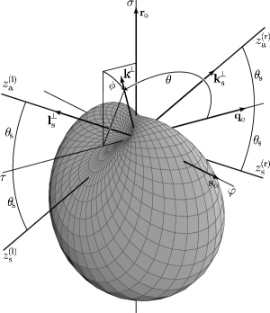
Figure 6: The magnitude of the leading terms of gravitational and electromagnetic fields, given by Eqs. (82) and (86), as a function of a direction from which the point $N_{\scriptscriptstyle{\boldsymbol{+}}}$ at infinity is approached — the directional pattern of radiation. The directions from the origin $N_{\scriptscriptstyle{\boldsymbol{+}}}$ of the diagram correspond to spatial directions in spacelike conformal infinity ${\mathcal{I}}^{+}$. The magnitude of the fields measured along a null geodesic with a tangent vector ${{\boldsymbol{\mathbf{k}}}}$ is drawn in the spatial direction ${-{{\boldsymbol{\mathbf{k}}}}^{\perp}}$ from which the geodesic arrives (i.e., the geodesic points into the spatial direction ${{\boldsymbol{\mathbf{k}}}}^{\perp}$). The angles ${\theta,\,\phi}$ parametrizing the spatial direction ${{\boldsymbol{\mathbf{k}}}}^{\perp}$ are measured from the axis ${{\boldsymbol{\mathbf{q}}}}_{\mathrm{o}}$, and around the axis ${{\boldsymbol{\mathbf{q}}}}_{\mathrm{o}}$ starting from the ${{{\boldsymbol{\mathbf{r}}}}_{\mathrm{o}}{\text{-}}{{\boldsymbol{\mathbf{q}}}}_{\mathrm{o}}}$ plane, respectively. The special geodesics in principal null directions ${{\boldsymbol{\mathbf{k}}}}_{\mathrm{s}}$ and ${{\boldsymbol{\mathbf{l}}}}_{\mathrm{s}}$, i.e., the null geodesics coming from the “left” black hole and the “right” black hole (pointing “from the sources”), are denoted by $z^{{(\mathrm{l})}}_{{\mathrm{s}}}$ and $z^{{(\mathrm{r})}}_{{\mathrm{s}}}$. They approach the point $N_{\scriptscriptstyle{\boldsymbol{+}}}$ at infinity along the spatial directions ${{\boldsymbol{\mathbf{k}}}}_{\mathrm{s}}^{\perp}$ and ${{\boldsymbol{\mathbf{l}}}}_{\mathrm{s}}^{\perp}$. On the other hand, $z^{{(\mathrm{r})}}_{{\mathrm{a}}}$ and $z^{{(\mathrm{l})}}_{{\mathrm{a}}}$ are “antipodal” null geodesics approaching the infinity along the spatial directions ${-{{\boldsymbol{\mathbf{k}}}}_{\mathrm{s}}^{\perp}}$, ${-{{\boldsymbol{\mathbf{l}}}}_{\mathrm{s}}^{\perp}}$, opposite to that of $z^{{(\mathrm{l})}}_{{\mathrm{s}}}$ and $z^{{(\mathrm{r})}}_{{\mathrm{s}}}$, respectively. The leading radiative term of the fields completely vanishes along these antipodal geodesics.

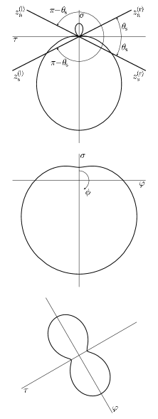
Figure 7: The particular sections ${\tau{\text{-}}\sigma}$, ${\sigma{\text{-}}\varphi}$ and ${\tau{\text{-}}\varphi}$ of the directional pattern of radiation shown in Fig. 6. The oriented angles $\theta$ of the spatial directions of the geodesics from sources (${\theta=\theta_{\mathrm{s}}}$ and ${\theta=\pi\!-\theta_{\mathrm{s}}}$, ${\phi=0}$) and of the antipodal geodesics (${\theta=\theta_{\mathrm{s}}}$ and ${\theta=\pi\!-\theta_{\mathrm{s}}}$, ${\phi=\pi}$) are indicated.

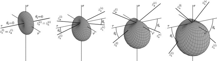
Figure 8: The directional pattern of radiation from Fig. 6 for different values of the angular parameter $\theta_{\mathrm{s}}$. Because the directional dependence Eq. (87) of the gravitational and electromagnetic radiation depends only on this single parameter $\theta_{\mathrm{s}}$ given by (40), both changes of a position $N_{\scriptscriptstyle{\boldsymbol{+}}}$ at infinity ${\mathcal{I}}^{+}$ and changes of the physical parameters $m$, $e$, $A$, and $\Lambda$ manifest only through a change of the angle $\theta_{\mathrm{s}}$. The diagrams with different values of $\theta_{\mathrm{s}}$ can thus be interpreted either as the directional patterns at different points of infinity ${\mathcal{I}}^{+}$, or as the directional characteristics at “the same” point (with fixed values of the metric functions ${\mathcal{F}}$ and ${\mathcal{G}}$), but in spacetimes with, for example, different acceleration of the black holes.

The invariant physical quantity ${\left\lvert\Psi^{{\mathrm{i}}}_{4}\right\rvert}$ is thus

$$\begin{split}\left\lvert\Psi^{{\mathrm{i}}}_{4}\right\rvert&\approx\frac{3}{4}\frac{(m-2\,e^{2}A\,\xi_{\scriptscriptstyle{\boldsymbol{+}}})}{\gamma\,a_{\scriptscriptstyle\Lambda}^{2}\,\cos^{2}\theta_{\mathrm{s}}}\,\frac{1}{\eta}\\ &\;\;\times\Bigl{(}(\sin\theta+\sin\theta_{\mathrm{s}}\cos\phi)^{2}+\sin^{2}\theta_{\mathrm{s}}\cos^{2}\theta\sin^{2}\phi\Bigr{)}{\mbox{\;,}}\end{split}$$ (82)

where the angle $\theta_{\mathrm{s}}$ identifying the principal null directions at infinity is, thanks to Eqs. (40), (6), (13) and ${{\mathcal{E}}_{\scriptscriptstyle{\boldsymbol{+}}}=-1}$, given by

$$\sin\theta_{\mathrm{s}}=\sqrt{\frac{{\mathcal{G}}_{\scriptscriptstyle{\boldsymbol{+}}}a_{\scriptscriptstyle\Lambda}^{2}A^{2}}{1+{\mathcal{G}}_{\scriptscriptstyle{\boldsymbol{+}}}a_{\scriptscriptstyle\Lambda}^{2}A^{2}}}{\mbox{\;,\quad}}\frac{1}{\cos^{2}\theta_{\mathrm{s}}}=1+{\mathcal{G}}_{\scriptscriptstyle{\boldsymbol{+}}}a_{\scriptscriptstyle\Lambda}^{2}A^{2}{\mbox{\;.}}$$ (83)

Note that the term ${(m-2\,e^{2}A\,\xi_{\scriptscriptstyle{\boldsymbol{+}}})}$ in Eq. (82) is positive, which follows (although not immediately, see Appendix B) from the conditions (5).

Analogously, we obtain the components $\Phi^{{\mathrm{i}}}_{n}$ of the electromagnetic field in the parallelly transported null tetrad in the form

$$\Phi^{{\mathrm{i}}}_{n}\sim\frac{1}{\eta^{3-n}}{\mbox{\;,\quad}}n=0,\,1,\,2{\mbox{\;,}}$$ (84)

which also exhibits the peeling behavior. The leading term of the radiative component $\Phi^{{\mathrm{i}}}_{2}$ is asymptotically

$$\begin{split}\Phi^{{\mathrm{i}}}_{2}\approx&\frac{1}{2\sqrt{2}}\frac{e}{\gamma\,a_{\scriptscriptstyle\Lambda}\cos\theta_{\mathrm{s}}}\frac{1}{\eta}\,\\ &\,\times\bigl{(}\sin\theta+\sin\theta_{\mathrm{s}}\cos\phi-i\sin\theta_{\mathrm{s}}\cos\theta\sin\phi\bigr{)}{\mbox{\;.}}\end{split}$$ (85)

Similarly to the $\Psi^{{\mathrm{i}}}_{4}$ component, only the modulus of this expression is independent of a choice of the interpretation tetrad. Moreover, the square of modulus now has a clear physical meaning — it is exactly the leading term of the magnitude of the Poynting vector ${\boldsymbol{\mathbf{S}}}_{\mathrm{i}}$ in the parallelly transported frame defined with respect to the timelike vector ${{\boldsymbol{\mathbf{n}}}}_{\mathrm{i}}$. Thus, we obtain

$$\begin{split}4\pi\left\lvert{\boldsymbol{\mathbf{S}}}_{\mathrm{i}}\right\rvert&\approx\left\lvert\Phi^{{\mathrm{i}}}_{2}\right\rvert^{2}\approx\frac{1}{8}\frac{e^{2}}{\gamma^{2}\,a_{\scriptscriptstyle\Lambda}^{2}\cos^{2}\theta_{\mathrm{s}}}\frac{1}{\eta^{2}}\,\\ &\;\;\times\bigl{(}(\sin\theta+\sin\theta_{\mathrm{s}}\cos\phi)^{2}+\sin^{2}\theta_{\mathrm{s}}\cos^{2}\theta\sin^{2}\phi\bigr{)}{\mbox{\;.}}\end{split}$$ (86)

The direction of the Poynting vector ${\boldsymbol{\mathbf{S}}}_{\mathrm{i}}$ is asymptotically given by the vector ${{\boldsymbol{\mathbf{q}}}}_{\mathrm{i}}$. Interestingly, the dependence of ${\left\lvert\Psi^{{\mathrm{i}}}_{4}\right\rvert}$ and ${\left\lvert\Phi^{{\mathrm{i}}}_{2}\right\rvert^{2}}$ on the direction along which a point $N_{\scriptscriptstyle{\boldsymbol{+}}}$ at infinity ${\mathcal{I}}^{+}$ is approached (i.e., the dependence on angles $\theta$ and $\phi$) is exactly the same, namely,

$${\mathcal{A}}(\theta,\phi)=(\sin\theta+\sin\theta_{\mathrm{s}}\cos\phi)^{2}+\sin^{2}\theta_{\mathrm{s}}\cos^{2}\theta\sin^{2}\phi{\mbox{\;.}}$$ (87)

The angular dependence (87) for a fixed value of $\theta_{\mathrm{s}}$ which characterize the directional pattern of radiation at a given point of ${\mathcal{I}}^{+}$ is shown in Figs. 6 and 7, and for various $\theta_{\mathrm{s}}$ in Fig. 8.

Let us now discuss the main results (82) and (86). These expressions can be understood as a more detailed characterization of radiative fields near the spacelike conformal infinity, supplementing thus the peeling behavior (78), (84). It follows from (82), (85) that the dominant components of both fields decay asymptotically near ${\mathcal{I}}^{+}$, corresponding to ${r=\infty}$, as ${({\gamma\,\eta})^{-1}=r^{-1}}$. The electromagnetic field is proportional to the charge parameter $e$ whereas the gravitational field is proportional to the mass parameter $m$ modified, interestingly, by the term ${-2\,e^{2}A\,\xi_{\scriptscriptstyle{\boldsymbol{+}}}}$ which is a combination of electric charge and acceleration parameters, and the constant $\xi_{\scriptscriptstyle{\boldsymbol{+}}}$ denoting a specific point at infinity ${\mathcal{I}}^{+}$. Both the gravitational field ${\left\lvert\Psi^{{\mathrm{i}}}_{4}\right\rvert}$ and the electromagnetic Poynting vector $4\pi\,\left\lvert{\boldsymbol{\mathbf{S}}}_{\mathrm{i}}\right\rvert\approx\left\lvert\Phi^{{\mathrm{i}}}_{2}\right\rvert^{2}$ are proportional to ${a_{\scriptscriptstyle\Lambda}^{-2}=\frac{1}{3}\Lambda}$ (but they also depend implicitly on $\Lambda$ through the parameter $\theta_{\mathrm{s}}$, cf.  Eq. (83)). The radiation at ${\mathcal{I}}^{+}$ thus increases with a growing value of the cosmological constant $\Lambda$.

The angular dependence of the magnitude of radiation ${{\mathcal{A}}(\theta,\phi)}$ is presented in Figs. 6 and 8. Their grid is given by the coordinate lines ${\theta=\text{constant}}$ and ${\phi=\text{constant}}$, respectively. It is straightforward to investigate the behavior of the function ${{\mathcal{A}}(\theta,\phi)}$ for a fixed $\theta$. The minimal value is ${{\mathcal{A}}(\theta,\pi)=(\sin\theta-\sin\theta_{\mathrm{s}})^{2}}$, and the maximum is ${{\mathcal{A}}(\theta,0)=(\sin\theta+\sin\theta_{\mathrm{s}})^{2}}$. The global maximum ${{\mathcal{A}}=(1+\sin\theta)^{2}}$ occurs for ${\theta=\frac{\pi}{2}}$, ${\phi=0}$. The greatest magnitude of radiation thus arrives at infinity from the direction of ${{\boldsymbol{\mathbf{r}}}}_{\mathrm{o}}$. On the other hand, the minimal value ${{\mathcal{A}}=0}$ is obtained for ${\theta=\theta_{\mathrm{s}}}$, ${\phi=\pi}$ and ${\theta=\pi-\theta_{\mathrm{s}}}$, ${\phi=\pi}$. These are exactly the spatial directions ${-{{\boldsymbol{\mathbf{l}}}}_{\mathrm{s}}^{\perp}}$, ${-{{\boldsymbol{\mathbf{k}}}}_{\mathrm{s}}^{\perp}}$ of antipodal null geodesics $z^{{(\mathrm{l})}}_{{\mathrm{a}}}$ and $z^{{(\mathrm{r})}}_{{\mathrm{a}}}$, along which the radiation completely vanishes. The value of ${\mathcal{A}}$ along the geodesics $z^{{(\mathrm{l})}}_{{\mathrm{s}}}$ and $z^{{(\mathrm{r})}}_{{\mathrm{s}}}$ coming from the black holes in the directions ${{\boldsymbol{\mathbf{k}}}}_{\mathrm{s}}^{\perp}$ (${\theta=\theta_{\mathrm{s}},\phi=0}$) and ${{\boldsymbol{\mathbf{l}}}}_{\mathrm{s}}^{\perp}$ (${\theta=\pi-\theta_{\mathrm{s}}}$, ${\phi=0}$) is ${{\mathcal{A}}=4\sin^{2}\theta_{\mathrm{s}}}$. The value along the direction ${{\boldsymbol{\mathbf{q}}}}_{\mathrm{o}}$ (corresponding to ${\theta=0}$) is ${{\mathcal{A}}=\sin^{2}\theta_{\mathrm{s}}}$, and along ${{\boldsymbol{\mathbf{s}}}}_{\mathrm{o}}$ (${\theta=\frac{\pi}{2}}$, ${\phi=\frac{\pi}{2}}$) is ${{\mathcal{A}}=1}$.

Finally, it is interesting to observe that for a vanishing acceleration of the black holes, i.e., for ${A=0}$ which implies ${\theta_{\mathrm{s}}=0}$, we obtain

$$\left\lvert\Psi^{{\mathrm{i}}}_{4}\right\rvert \approx\frac{3}{4}\,\frac{m}{\gamma\,a_{\scriptscriptstyle\Lambda}^{2}}\,\frac{1}{\eta}\,\sin^{2}\theta{\mbox{\;,}}$$ (88)

$$\left\lvert\Phi^{{\mathrm{i}}}_{2}\right\rvert \approx\frac{1}{2\sqrt{2}}\frac{e}{\gamma\,a_{\scriptscriptstyle\Lambda}}\frac{1}{\eta}\,\sin\theta{\mbox{\;.}}$$

The angular dependence ${{\mathcal{A}}=\sin^{2}\theta}$ is now independent of $\phi$ so that the directional pattern is axially symmetric (see the diagram on the very left of Fig. 8). Moreover, the gravitational and electromagnetic fields decay as ${1/\eta}$ even in this case of nonaccelerated black holes if the fields are measured along a nonradial null geodesic (${\theta\neq 0,\pi}$). A generic observer thus detects radiation. This effect is intuitively caused by observer’s asymptotic motion relative to the “static” black holes. Only for special observers moving along null geodesics radially from the black holes (${\theta=0,\pi}$) the radiation vanishes as one would expect for “static” sources.

Interestingly, the angular dependence ${{\mathcal{A}}(\theta,\phi)}$ is exactly the same as that obtained in Bičák and Krtouš (2002) for test electromagnetic field of two accelerated charges in de Sitter space (note nt:FUACS ).

VI The radiation in the Robinson-Trautman framework

In this part we rederive the above results using the framework naturally adapted to the Robinson-Trautman coordinate system (14). This will not only provide us with an independent way of deriving the characteristic directional pattern of radiation generated by accelerated charged black holes in the asymptotically de Sitter universe, but opens a possibility to investigate even more general exact radiative solutions from the large and important Robinson-Trautman family.

We start again with investigation of asymptotic null geodesics approaching infinity ${\mathcal{I}}^{+}$, i.e., those for which ${r\to\infty}$. Assuming a natural expansion of these geodesics in powers of $\;{1/r}\;$ (rather than in the affine parameter ${1/\eta}$ as was done in the previous section),

$$\begin{gathered}\begin{aligned} \zeta&\approx\zeta_{\scriptscriptstyle{\boldsymbol{+}}}+\frac{c}{r}+\cdots{\mbox{\;,}}\\ u&\approx u_{\scriptscriptstyle{\boldsymbol{+}}}+\frac{d}{r}+\cdots{\mbox{\;,}}\end{aligned}\\ r(\eta)\to\infty\quad\text{as}\quad\eta\to\infty{\mbox{\;,}}\end{gathered}$$ (89)

where $\zeta_{\scriptscriptstyle{\boldsymbol{+}}}$, $u_{\scriptscriptstyle{\boldsymbol{+}}}$, $c$, $d$ are constants, the derivatives with respect to the affine parameter $\eta$ are

$$\dot{\zeta} \approx-\frac{\dot{r}}{r^{2}}\,c+\cdots{\mbox{\;,}}$$ (90)

$$\ddot{\zeta} \approx-\frac{\ddot{r}}{r^{2}}\Bigl{(}c+\cdots\Bigr{)}+\frac{{\dot{r}}^{2}}{r^{3}}\Bigl{(}2c+\cdots\Bigr{)}{\mbox{\;.}}$$

The expressions for $\dot{u}$, $\ddot{u}$ are obtained from (90) by replacing $c$ with $d$. Similarly, we may expand the metric functions and other quantities. Using Eqs. (89) and (90) and the Christoffel symbols (157), the geodesic equations in the highest order read

$$c\frac{\ddot{r}}{r}=0{\mbox{\;,\quad}}d\frac{\ddot{r}}{r}=\mathcal{N}\,\frac{\dot{r}^{2}}{r^{2}}{\mbox{\;,\quad}}a_{\scriptscriptstyle\Lambda}^{2}\frac{\ddot{r}}{r}=-\mathcal{N}\,\frac{\dot{r}^{2}}{r^{2}}{\mbox{\;,}}$$ (91)

where

$$\mathcal{N}=2P_{\scriptscriptstyle{\boldsymbol{+}}}^{-2}c\bar{c}+2d+a_{\scriptscriptstyle\Lambda}^{-2}d^{2}{\mbox{\;,}}$$ (92)

$P_{\scriptscriptstyle{\boldsymbol{+}}}$ being the asymptotic value of $P$ at the point $N_{\scriptscriptstyle{\boldsymbol{+}}}$ at infinity. However, a normalization of the tangent vector for null geodesics requires

$$\mathcal{N}=0{\mbox{\;.}}$$ (93)

Consequently, the asymptotic form of the null geodesics approaching ${\mathcal{I}}^{+}$ is

$$\begin{gathered}r\approx\gamma\,\eta{\mbox{\;,\quad}}\zeta\approx\zeta_{\scriptscriptstyle{\boldsymbol{+}}}+\frac{c}{r}{\mbox{\;,\quad}}u\approx u_{\scriptscriptstyle{\boldsymbol{+}}}+\frac{d}{r}{\mbox{\;,}}\\ \frac{Dz}{d\eta}=\gamma\Bigl{(}{{\boldsymbol{\mathbf{\partial}}}_{r}}-\frac{c}{r^{2}}\,{{\boldsymbol{\mathbf{\partial}}}_{\zeta}}-\frac{\bar{c}}{r^{2}}\,{{\boldsymbol{\mathbf{\partial}}}_{\bar{\zeta}}}-\frac{d}{r^{2}}\,{{\boldsymbol{\mathbf{\partial}}}_{u}}\Bigr{)}{\mbox{\;,}}\end{gathered}$$ (94)

where the constant $\gamma$ can be identified with that introduced in Eq. (68), $\zeta_{\scriptscriptstyle{\boldsymbol{+}}}$, $u_{\scriptscriptstyle{\boldsymbol{+}}}$ specify the point $N_{\scriptscriptstyle{\boldsymbol{+}}}$ on ${\mathcal{I}}^{+}$ towards which the particular geodesic is approaching, and $c$, $d$ are parameters representing the direction along which $N_{\scriptscriptstyle{\boldsymbol{+}}}$ is reached. In fact, this direction is basically parametrized just by the complex constant $c$ since, using relations (93), (92), $d$ is then given as ${d=-a_{\scriptscriptstyle\Lambda}^{2}\bigl{(}\,1\pm\sqrt{1-2a_{\scriptscriptstyle\Lambda}^{-2}P_{\scriptscriptstyle{\boldsymbol{+}}}^{-2}c\bar{c}}\;\bigr{)}}$. For a particular $c$, there are thus only two real values of $d$ which represent two possible different orientations with which the null geodesics may approach ${\mathcal{I}}^{+}$ in the given spatial direction. In particular, for the special choice ${c=0}$ we obtain ${d=0}$ and ${d=-2a_{\scriptscriptstyle\Lambda}^{2}}$. The first corresponds exactly to the privileged principal null direction along ${{\boldsymbol{\mathbf{k}}}}_{\mathrm{s}}$ “from the source” (i.e., the null geodesic $z^{{(\mathrm{l})}}_{{\mathrm{s}}}$ along the spatial direction ${{\boldsymbol{\mathbf{k}}}}_{\mathrm{s}}^{\perp}$), the second to an opposite orientation of this direction “away from the source” (the “antipodal” null geodesic $z^{{(\mathrm{r})}}_{{\mathrm{a}}}$ along ${-{{\boldsymbol{\mathbf{k}}}}_{\mathrm{s}}^{\perp}}$), see Fig. 6.

In order to find the behavior of radiation near ${\mathcal{I}}^{+}$ we again have to set up the interpretation tetrad transported parallelly along a general asymptotic null geodesic, and project the Weyl tensor and the tensor of electromagnetic field onto this tetrad. We start with the Robinson-Trautman null tetrad (56), naturally adapted to the Robinson-Trautman coordinate system (14). We have seen in Section IV that the vector ${{\boldsymbol{\mathbf{k}}}}_{\scriptscriptstyle\mathrm{RT}}$ is oriented along one of the principal null direction, namely, ${{\boldsymbol{\mathbf{k}}}}_{\mathrm{s}}$, and (as we will see in Section VII) the tetrad (56) is parallelly transported along the algebraically special geodesics. In this standard tetrad the only nontrivial components $\Psi^{{\scriptscriptstyle\mathrm{RT}}}_{n}$ and $\Phi^{{\scriptscriptstyle\mathrm{RT}}}_{n}$, which represent the gravitational and electromagnetic field, are given by Eqs. (62) and (63). Let us now perform two subsequent null rotations and a boost of this Robinson-Trautman null tetrad (56). We first apply Eq. (185), then (182), and finally (188) with the parameters

$$K =-\frac{c}{(1+\frac{1}{2}a_{\scriptscriptstyle\Lambda}^{-2}d)\,P\,r}{\mbox{\;,\quad}}$$ (95)

$$L =\frac{c\,r}{2a_{\scriptscriptstyle\Lambda}^{2}P}{\mbox{\;,\quad}}$$

$$B =1+\textstyle{\frac{1}{2}}a_{\scriptscriptstyle\Lambda}^{-2}d{\mbox{\;,\quad}}\Phi=0{\mbox{\;.}}$$

The resulting null tetrad, using relation (93), then takes the following asymptotic form as ${r\to\infty}$:

$${{\boldsymbol{\mathbf{k}}}}_{\mathrm{i}} \approx\left({{\boldsymbol{\mathbf{\partial}}}_{r}}-\frac{c}{r^{2}}\,{{\boldsymbol{\mathbf{\partial}}}_{\zeta}}-\frac{\bar{c}}{r^{2}}\,{{\boldsymbol{\mathbf{\partial}}}_{\bar{\zeta}}}-\frac{d}{r^{2}}\,{{\boldsymbol{\mathbf{\partial}}}_{u}}\right){\mbox{\;,}}$$ (96)

$${{\boldsymbol{\mathbf{l}}}}_{\mathrm{i}} \approx\frac{r^{2}}{2a_{\scriptscriptstyle\Lambda}^{2}}\left({{\boldsymbol{\mathbf{\partial}}}_{r}}+\frac{c}{r^{2}}\,{{\boldsymbol{\mathbf{\partial}}}_{\zeta}}+\frac{\bar{c}}{r^{2}}\,{{\boldsymbol{\mathbf{\partial}}}_{\bar{\zeta}}}+\frac{d+2a_{\scriptscriptstyle\Lambda}^{2}}{r^{2}}\,{{\boldsymbol{\mathbf{\partial}}}_{u}}\right){\mbox{\;,}}$$

$${{\boldsymbol{\mathbf{m}}}}_{\mathrm{i}} \approx\frac{P}{r}\left(\,\frac{c\,d}{2a_{\scriptscriptstyle\Lambda}^{2}\bar{c}}\,{{\boldsymbol{\mathbf{\partial}}}_{\zeta}}+(1+{\textstyle\frac{1}{2}}a_{\scriptscriptstyle\Lambda}^{-2}d)\,{{\boldsymbol{\mathbf{\partial}}}_{\bar{\zeta}}}-\frac{c}{P^{2}}\,{{\boldsymbol{\mathbf{\partial}}}_{u}}\right){\mbox{\;,}}$$

$${\bar{{\boldsymbol{\mathbf{m}}}}}_{\mathrm{i}} \approx\frac{P}{r}\left(\,(1+{\textstyle\frac{1}{2}}a_{\scriptscriptstyle\Lambda}^{-2}d)\,{{\boldsymbol{\mathbf{\partial}}}_{\zeta}}+\frac{\bar{c}\,d}{2a_{\scriptscriptstyle\Lambda}^{2}c}\,{{\boldsymbol{\mathbf{\partial}}}_{\bar{\zeta}}}-\frac{\bar{c}}{P^{2}}\,{{\boldsymbol{\mathbf{\partial}}}_{u}}\right){\mbox{\;.}}$$

Obviously, the above vector ${{\boldsymbol{\mathbf{k}}}}_{\mathrm{i}}$ is tangent to a general asymptotic null geodesics (94). Moreover, the tetrad is chosen in such a way that the timelike unit vector orthogonal to ${\mathcal{I}}^{+}$

$${{\boldsymbol{\mathbf{n}}}}_{\mathrm{o}}=\frac{1}{\sqrt{-H}}\,\left(-H\,{{\boldsymbol{\mathbf{\partial}}}_{r}}+{{\boldsymbol{\mathbf{\partial}}}_{u}}\,\right)\approx\frac{r}{a_{\scriptscriptstyle\Lambda}}\,{{\boldsymbol{\mathbf{\partial}}}_{r}}+\frac{a_{\scriptscriptstyle\Lambda}}{r}\,{{\boldsymbol{\mathbf{\partial}}}_{u}}{\mbox{\;,}}$$ (97)

introduced in Eq. (35), belongs to the plane spanned by the two null vectors ${{\boldsymbol{\mathbf{k}}}}_{\mathrm{i}}$ and ${{\boldsymbol{\mathbf{l}}}}_{\mathrm{i}}$. Indeed,

$${{\boldsymbol{\mathbf{n}}}}_{\mathrm{o}}\approx\frac{1}{\sqrt{2}}\Bigl{(}\frac{r}{{\sqrt{2}}\,a_{\scriptscriptstyle\Lambda}}\,{{\boldsymbol{\mathbf{k}}}}_{\mathrm{i}}+\frac{{\sqrt{2}}\,a_{\scriptscriptstyle\Lambda}}{r}\,{{\boldsymbol{\mathbf{l}}}}_{\mathrm{i}}\Bigr{)}{\mbox{\;.}}$$ (98)

Note that this choice corresponds to a boost Eq. (188) which becomes unbounded as ${r\to\infty}$.

As discussed in the previous section, in order to compare the radiation for all null geodesics approaching the given point at de Sitter-like infinity ${\mathcal{I}}^{+}$, it is necessary to introduce a unique and universal normalization of the affine parameter $\eta$ and of the vector ${{\boldsymbol{\mathbf{k}}}}_{\mathrm{i}}$. We concluded that a natural and also the most convenient choice is to keep the parameter $\gamma$ fixed (see discussion near Eq. (69)) and to require Eq. (72). These conditions are obviously satisfied by Eq. (96), cf.  Eq. (94). Therefore, the tetrad (96) is exactly the interpretation tetrad suitable for analysis of behavior of fields on ${\mathcal{I}}^{+}$.

Now we perform a projection of the above null tetrad onto the spacelike infinity ${\mathcal{I}}^{+}$. These projections ${{{\boldsymbol{\mathbf{k}}}}_{\mathrm{i}}^{\perp},\,{{\boldsymbol{\mathbf{l}}}}_{\mathrm{i}}^{\perp},\,{{\boldsymbol{\mathbf{m}}}}_{\mathrm{i}}^{\perp}}$ (cf. Eq. (38)) are

$$\begin{gathered}{{\boldsymbol{\mathbf{k}}}}_{\mathrm{i}}^{\perp}\approx-\frac{1}{r^{2}}\,\Bigl{(}\,c\,{{\boldsymbol{\mathbf{\partial}}}_{\zeta}}+\bar{c}\,{{\boldsymbol{\mathbf{\partial}}}_{\bar{\zeta}}}+(d+a_{\scriptscriptstyle\Lambda}^{2})\,{{\boldsymbol{\mathbf{\partial}}}_{u}}\,\Bigr{)}{\mbox{\;,}}\\ {{\boldsymbol{\mathbf{l}}}}_{\mathrm{i}}^{\perp}\approx-\frac{r^{2}}{2a_{\scriptscriptstyle\Lambda}^{2}}\,{{\boldsymbol{\mathbf{k}}}}_{\mathrm{i}}^{\perp}{\mbox{\;,\quad}}{{\boldsymbol{\mathbf{m}}}}_{\mathrm{i}}^{\perp}={{\boldsymbol{\mathbf{m}}}}_{\mathrm{i}}{\mbox{\;,\quad}}{\bar{{\boldsymbol{\mathbf{m}}}}}_{\mathrm{i}}^{\perp}={\bar{{\boldsymbol{\mathbf{m}}}}}_{\mathrm{i}}{\mbox{\;.}}\end{gathered}$$ (99)

The radiation approaching ${\mathcal{I}}^{+}$ along the null vector ${{\boldsymbol{\mathbf{k}}}}_{\mathrm{i}}$ propagates in the spatial direction ${{{\boldsymbol{\mathbf{k}}}}_{\mathrm{i}}^{\perp}\propto{{\boldsymbol{\mathbf{q}}}}_{\mathrm{r}}}$. Imposing the normalization condition ${{{\boldsymbol{\mathbf{q}}}}_{\mathrm{r}}\mathbin{\boldsymbol{\cdot}}{{\boldsymbol{\mathbf{q}}}}_{\mathrm{r}}=1}$, the unit vector of the radiation direction thus takes the form

$${{\boldsymbol{\mathbf{q}}}}_{\mathrm{r}}\approx-\frac{1}{a_{\scriptscriptstyle\Lambda}\,r}\,\Bigl{(}\,c\,{{\boldsymbol{\mathbf{\partial}}}_{\zeta}}+\bar{c}\,{{\boldsymbol{\mathbf{\partial}}}_{\bar{\zeta}}}+(d+a_{\scriptscriptstyle\Lambda}^{2})\,{{\boldsymbol{\mathbf{\partial}}}_{u}}\,\Bigr{)}{\mbox{\;.}}$$ (100)

Of course, this vector is identical to the vector ${{\boldsymbol{\mathbf{q}}}}_{\mathrm{r}}$ introduced previously in Eq. (54). Using Eqs. (176f)–(176h), (35), and (40) we obtain

$${{\boldsymbol{\mathbf{\partial}}}_{\zeta}} =\frac{1}{\sqrt{2}}\,\frac{r}{P}\,\left(-\sin\theta_{\mathrm{s}}\,{{\boldsymbol{\mathbf{q}}}}_{\mathrm{o}}+\cos\theta_{\mathrm{s}}\,{{\boldsymbol{\mathbf{r}}}}_{\mathrm{o}}+i\,{{\boldsymbol{\mathbf{s}}}}_{\mathrm{o}}\,\right){\mbox{\;,}}$$ (101)

$${{\boldsymbol{\mathbf{\partial}}}_{u}} =-\sqrt{-H}\,\left(\,\cos\theta_{\mathrm{s}}\,{{\boldsymbol{\mathbf{q}}}}_{\mathrm{o}}+\sin\theta_{\mathrm{s}}\,{{\boldsymbol{\mathbf{r}}}}_{\mathrm{o}}\,\right){\mbox{\;,}}$$

$${{\boldsymbol{\mathbf{\partial}}}_{r}} =\frac{1}{\sqrt{-H}}\,\left(\,{{\boldsymbol{\mathbf{n}}}}_{\mathrm{o}}+\cos\theta_{\mathrm{s}}\,{{\boldsymbol{\mathbf{q}}}}_{\mathrm{o}}+\sin\theta_{\mathrm{s}}\,{{\boldsymbol{\mathbf{r}}}}_{\mathrm{o}}\,\right){\mbox{\;.}}$$

Substituting this into Eq. (100), using ${{\mathcal{E}}_{\scriptscriptstyle{\boldsymbol{+}}}=-1}$, and comparing with the expression (54), we obtain the following relation between the Robinson-Trautman parameters $\,c$, $d\,$ and the angles $\,{\theta,\,\phi}\,$

$$\frac{c+\bar{c}}{\sqrt{2}\,a_{\scriptscriptstyle\Lambda}P_{\scriptscriptstyle{\boldsymbol{+}}}} ={\mspace{14.5mu}}\sin\theta_{\mathrm{s}}\cos\theta-\cos\theta_{\mathrm{s}}\sin\theta\cos\phi{\mbox{\;,}}$$ (102)

$$i\frac{c-\bar{c}}{\sqrt{2}\,a_{\scriptscriptstyle\Lambda}P_{\scriptscriptstyle{\boldsymbol{+}}}} =-\sin\theta\sin\phi{\mbox{\;,}}$$

$$1+a_{\scriptscriptstyle\Lambda}^{-2}d ={\mspace{14.5mu}}\cos\theta_{\mathrm{s}}\cos\theta+\sin\theta_{\mathrm{s}}\sin\theta\cos\phi{\mbox{\;.}}$$

Of course, this parametrization identically satisfies the normalization condition (93). Moreover, it can now be demonstrated that the above null tetrad (96) is in fact identical to the parallelly transported tetrad (75), except for the transverse vector ${{\boldsymbol{\mathbf{m}}}}_{\mathrm{i}}$, which was previously defined as ${{{\boldsymbol{\mathbf{m}}}}_{\mathrm{i}}\approx{{\boldsymbol{\mathbf{m}}}}_{\mathrm{r}}}$, ${{\boldsymbol{\mathbf{m}}}}_{\mathrm{r}}$ given by Eq. (179) (cf.  Eqs. (54), (23)). Such a vector is related to the vector ${{\boldsymbol{\mathbf{m}}}}_{\mathrm{i}}$ adapted to the Robinson-Trautman framework (96) by the spatial rotation (188), ${{{\boldsymbol{\mathbf{m}}}}_{\mathrm{i}}=\exp(-i\phi_{\mathrm{i}})\,{{\boldsymbol{\mathbf{m}}}}_{\mathrm{r}}}$, where the rotation angle $\phi_{\mathrm{i}}$ is given by

$$\begin{gathered}\begin{aligned} \sin\phi_{\mathrm{i}}&=\frac{(\,\cos\theta_{\mathrm{s}}+\cos\theta\,)\sin\phi}{1+\cos\theta_{\mathrm{s}}\cos\theta+\sin\theta_{\mathrm{s}}\sin\theta\cos\phi}{\mbox{\;,}}\\ \cos\phi_{\mathrm{i}}&=\frac{\sin\theta_{\mathrm{s}}\sin\theta+(1+\cos\theta_{\mathrm{s}}\cos\theta\,)\cos\phi}{1+\cos\theta_{\mathrm{s}}\cos\theta+\sin\theta_{\mathrm{s}}\sin\theta\cos\phi}{\mbox{\;,}}\end{aligned}\\ \exp(i\phi_{\mathrm{i}})=\frac{\exp(i\phi)\cos\frac{\theta_{\mathrm{s}}}{2}\cos\frac{\theta}{2}+\sin\frac{\theta_{\mathrm{s}}}{2}\sin\frac{\theta}{2}}{\cos\frac{\theta_{\mathrm{s}}}{2}\cos\frac{\theta}{2}+\exp(i\phi)\sin\frac{\theta_{\mathrm{s}}}{2}\sin\frac{\theta}{2}}{\mbox{\;.}}\end{gathered}$$ (103)

Finally, we calculate the leading components of the gravitational and electromagnetic fields in the interpretation frame (96) asymptotically close to infinity ${\mathcal{I}}^{+}$. As we have said, the Lorentz transformation from the tetrad (56) to the tetrad (96) is given by two subsequent null rotations and the boost with the parameters given by Eq. (95). Starting with the components (62) in the standard Robinson-Trautman frame, using Eqs. (186), (183), (190) and (187), (184), (191), we obtain after somewhat lengthy calculation

$$\Psi^{{\mathrm{i}}}_{4} \approx-\frac{3A^{2}(m-2e^{2}A\,\xi_{\scriptscriptstyle{\boldsymbol{+}}})}{r\,P_{\scriptscriptstyle{\boldsymbol{+}}}^{2}}\,\left(1-\frac{1}{\sqrt{2}\,a_{\scriptscriptstyle\Lambda}^{2}A}\,\bar{c}+{\frac{1}{2a_{\scriptscriptstyle\Lambda}^{2}}}\,d\right)^{2}{\mbox{\;,}}$$

$$\Phi^{{\mathrm{i}}}_{2} \approx\ \frac{e\,A}{\sqrt{2}\,r\,P_{\scriptscriptstyle{\boldsymbol{+}}}}\,\left(1-\frac{1}{\sqrt{2}\,\,a_{\scriptscriptstyle\Lambda}^{2}A}\,\bar{c}+{\frac{1}{2a_{\scriptscriptstyle\Lambda}^{2}}}\,d\right){\mbox{\;.}}$$ (104)

Substituting from Eq. (102) for the parameters $c$ and $d$, and using Eqs. (83) and (15) we get

$$\Psi^{{\mathrm{i}}}_{4} \approx-\frac{3}{4}\frac{(m-2e^{2}A\,\xi_{\scriptscriptstyle{\boldsymbol{+}}})}{a_{\scriptscriptstyle\Lambda}^{2}\,r\,\cos^{2}\theta_{\mathrm{s}}}$$ (105)

$$\;\times\!\left(\,\sin\theta_{\mathrm{s}}+\sin\theta\cos\phi+i\cos\theta_{\mathrm{s}}\sin\theta\sin\phi\,\right)^{2}{\mbox{\;,}}$$

$$\Phi^{{\mathrm{i}}}_{2} \approx\frac{1}{2\sqrt{2}}\frac{e}{a_{\scriptscriptstyle\Lambda}\,r\,\cos\theta_{\mathrm{s}}}$$

$$\;\times\!\left(\,\sin\theta_{\mathrm{s}}+\sin\theta\cos\phi+i\cos\theta_{\mathrm{s}}\sin\theta\sin\phi\,\right){\mbox{\;,}}$$

We should have recovered the previous results (79) and (85). Comparing them we find that the expressions differ in the angular part. However, this is a consequence of the difference of interpretation tetrads used in the previous and in this sections. The results are, in fact, identical after performing a spatial rotation (188) with the angular parameter $\phi_{\mathrm{i}}$ given by Eq. (103). This changes the phase of the components according to Eqs. (190), (191), and we obtain ${\Psi^{{\mathrm{i}}}_{4}=\exp(2i\phi_{\mathrm{i}})\,\Psi^{{\mathrm{i}}}_{4}}$, ${\Phi^{{\mathrm{i}}}_{2}=\exp(i\phi_{\mathrm{i}})\,\Phi^{{\mathrm{i}}}_{2}}$, where the left-hand side is given by Eq. (105), and the right hand side by Eqs. (79), (85). Both results are thus equivalent.

The tetrads (75) and (96) have been introduced in a way natural to each specific approach. The fact that they differ in definitions of the vector ${{\boldsymbol{\mathbf{m}}}}_{\mathrm{i}}$ documents what we have already discussed above: there is no canonical way how to choose the interpretation tetrad. It also means that the phase of the results (79), (85), or (105) is not physical. Invariant information, independent of a choice of the interpretation tetrad, is contained in the modulus of the tetrad components of the fields. Obviously, the magnitudes of the field components (105) are the same as the results (82) and (86) derived previously.

VII Radiation along the algebraically special null directions

In the final section we concentrate on a family of special geodesics ${z^{{(\mathrm{l})}}_{{\mathrm{s}}}}$ approaching infinity ${\mathcal{I}}^{+}$ along principal null direction ${{\boldsymbol{\mathbf{k}}}}_{\mathrm{s}}$, and investigate the fields with respect to the corresponding interpretation tetrad. Using Eqs. (157) it is straightforward to observe that the coordinate lines

$$u=u_{\scriptscriptstyle{\boldsymbol{+}}}=\text{constant}{\mbox{\;,\quad}}\zeta=\zeta_{\scriptscriptstyle{\boldsymbol{+}}}=\text{constant}$$ (106)

(i.e., also ${\xi=\text{constant}}$, ${\varphi=\text{constant}}$) are null geodesics, $r$ is their affine parameter, and the tangent vector is ${{{\boldsymbol{\mathbf{k}}}}_{\scriptscriptstyle\mathrm{RT}}={{\boldsymbol{\mathbf{\partial}}}_{r}}}$. (For simplicity, in this section we use the affine parameter $r$, a general affine parameter $\eta$ can be introduced by a trivial rescaling ${r=\gamma\,\eta}$, cf.  Eq. (68).) The geodesics ${z^{{(\mathrm{l})}}_{{\mathrm{s}}}(r)}$ emanate “radially” from the “left” black hole up to the infinity (similarly we could investigate analogous geodesics ${z^{{(\mathrm{r})}}_{{\mathrm{s}}}}$ along ${{\boldsymbol{\mathbf{l}}}}_{\mathrm{s}}$ from the “right” black hole). As we have seen in Section IV (cf.  Eq. (57) and the subsequent discussion), the tangent vector ${{\boldsymbol{\mathbf{k}}}}_{\scriptscriptstyle\mathrm{RT}}$ is oriented along the principal null direction ${{\boldsymbol{\mathbf{k}}}}_{\mathrm{s}}$. These geodesics thus approach the infinity from the specific spatial direction characterized by the angles

$$\theta=\theta_{\mathrm{s}}{\mbox{\;,\quad}}\phi=0{\mbox{\;,}}$$ (107)

or by the parameters ${c=0}$, ${d=0}$ (see Eq. (102)).

Moreover, in such a case we can identify explicitly the parallelly transported interpretation tetrad — it can easily be shown using Eqs. (157) that the Robinson-Trautman tetrad (56) is parallelly transported along ${z^{{(\mathrm{l})}}_{{\mathrm{s}}}(r)}$, i.e.,

$${{\boldsymbol{\mathbf{k}}}}_{\scriptscriptstyle\mathrm{RT}}\cdot\nabla{{\boldsymbol{\mathbf{k}}}}_{\scriptscriptstyle\mathrm{RT}}=0{\mbox{\;,\quad}}{{\boldsymbol{\mathbf{k}}}}_{\scriptscriptstyle\mathrm{RT}}\cdot\nabla{{\boldsymbol{\mathbf{l}}}}_{\scriptscriptstyle\mathrm{RT}}=0{\mbox{\;,\quad}}{{\boldsymbol{\mathbf{k}}}}_{\scriptscriptstyle\mathrm{RT}}\cdot\nabla{{\boldsymbol{\mathbf{m}}}}_{\scriptscriptstyle\mathrm{RT}}=0{\mbox{\;.}}$$ (108)

We can thus set the interpretation tetrad

$$({{\boldsymbol{\mathbf{k}}}}_{\mathrm{i}},\,{{\boldsymbol{\mathbf{l}}}}_{\mathrm{i}},\,{{\boldsymbol{\mathbf{m}}}}_{\mathrm{i}},\,{\bar{{\boldsymbol{\mathbf{m}}}}}_{\mathrm{i}})\equiv({{\boldsymbol{\mathbf{k}}}}_{\scriptscriptstyle\mathrm{RT}},\,{{\boldsymbol{\mathbf{l}}}}_{\scriptscriptstyle\mathrm{RT}},\,{{\boldsymbol{\mathbf{m}}}}_{\scriptscriptstyle\mathrm{RT}},\,{\bar{{\boldsymbol{\mathbf{m}}}}}_{\scriptscriptstyle\mathrm{RT}})$$ (109)

in the whole spacetime, not only asymptotically near ${\mathcal{I}}^{+}$, as in Eq. (96) for ${c=0}$, ${d=0}$. As follows from Eqs. (62) and (63), all components of gravitational and electromagnetic fields are explicitly

$$\Psi^{{\mathrm{i}}}_{4} =-3\,\Bigl{(}m-2\,e^{2}A\,\xi-\frac{e^{2}}{r}\Bigr{)}\,A^{2}{\mathcal{G}}\,\frac{1}{r}{\mbox{\;,}}$$ (110)

$$\Psi^{{\mathrm{i}}}_{3} =\frac{3}{\sqrt{2}}\,\Bigl{(}m-2\,e^{2}A\,\xi-\frac{e^{2}}{r}\Bigr{)}\,A\sqrt{{\mathcal{G}}}\,\frac{1}{r^{2}}{\mbox{\;,}}$$

$$\Psi^{{\mathrm{i}}}_{2} =-\Bigl{(}m-2\,e^{2}A\,\xi-\frac{e^{2}}{r}\Bigr{)}\,\frac{1}{r^{3}}{\mbox{\;,\quad}}\Psi^{{\mathrm{i}}}_{1}=\Psi^{{\mathrm{i}}}_{0}=0{\mbox{\;,}}$$

and

$$\Phi^{{\mathrm{i}}}_{2}=\frac{e\,A\sqrt{{\mathcal{G}}}}{\sqrt{2}}\,\frac{1}{r}{\mbox{\;,\quad}}\Phi^{{\mathrm{i}}}_{1}=-\frac{e}{2}\,\frac{1}{r^{2}}{\mbox{\;,\quad}}\Phi^{{\mathrm{i}}}_{0}=0{\mbox{\;.}}$$ (111)

Clearly, the leading terms in the ${1/r}$ expansion give the previous general asymptotical results (82) and (86) with ${\theta,\,\phi}$ specified by Eq. (107), and ${r=\gamma\,\eta}$. In the case of de Sitter spacetime (${m=0}$, ${e=0}$) the field components identically vanish, in the general case the fields have a radiative character (${\sim 1/r}$) except for a vanishing acceleration $A$ and/or for ${{\mathcal{G}}_{\scriptscriptstyle{\boldsymbol{+}}}=0}$. The “static” case ${A=0}$ has been already discussed after Eq. (88). The case ${{\mathcal{G}}_{\scriptscriptstyle{\boldsymbol{+}}}=0}$ corresponds to observers located at the privileged position — on the axes ${\xi=\xi_{1}}$ and ${\xi=\xi_{2}}$. This is analogous to the well-known situation of an electromagnetic field of accelerated test charges in flat spacetime which is also not radiative along the axis of symmetry.

Let us note that in this case the affine parameter $r$ coincides, in fact, both with the luminosity distance and the parallax distance for the congurence of the above null geodesics — as for any Robinson-Trautman spacetime described by the metric (14). Indeed, the luminosity distance $r_{\!\scriptscriptstyle\mathrm{L}}$ is related to the affine parameter $r$ by the relation Sachs (1962)

$$\frac{dr_{\!\scriptscriptstyle\mathrm{L}}}{dr}=\frac{1}{2}\,r_{\!\scriptscriptstyle\mathrm{L}}\,\nabla\cdot{{\boldsymbol{\mathbf{k}}}}_{\scriptscriptstyle\mathrm{RT}}{\mbox{\;.}}$$ (112)

Thanks to Eqs. (157) one obtains ${\frac{1}{2}\nabla\cdot{{\boldsymbol{\mathbf{k}}}}_{\scriptscriptstyle\mathrm{RT}}=1/r}$, and thus ${r_{\!\scriptscriptstyle\mathrm{L}}=r}$. This means that the radiative ${1/r}$ fall-off of the fields is naturally measurable (even locally) by observers moving radially to infinity, using both the parallax and the luminosity methods for determining the distance.

In the previous sections, when we studied the radiation along general geodesics, we have been able to fix the interpretation tetrad only asymptotically, by specifying appropriate final conditions at infinity (see Eq. (71), (75) and the discussion nearby). For the special family of geodesics (106) discussed here we can specify the interpretation tetrad by setting the initial conditions anywhere in the finite region inside the spacetime. Because any point at infinity ${\mathcal{I}}^{+}$ is only reached by one algebraically special geodesic $z^{{(\mathrm{l})}}_{{\mathrm{s}}}$ from the “left” black hole, this does not allow us to study the directional pattern of radiation with respect to the interpretation tetrad fixed by these explicit initial conditions. However, we can study the standard positional pattern of radiation along these special geodesics — the dependence of radiation on the position of asymptotic point $N_{\scriptscriptstyle{\boldsymbol{+}}}$ in the infinity.

The initial conditions for interpretation tetrad inside a finite region of the spacetime can be chosen in many different ways, e.g., using some natural tetrad on a spacelike hypersurface (“initial instant of time”, note nt:FUACSincond ), on a “surface of sources”, on a special null hypersurface, etc. Obviously, geometrically privileged locations where we can specify such initial conditions are horizons, in particular the cosmological horizon ${\upsilon=\upsilon_{\mathrm{c}}}$, or the outer horizon ${\upsilon=\upsilon_{\mathrm{o}}}$ of the “left” black hole. The former one (its “future” half) forms a (past) boundary of the domain in which any observer has to reach the future infinity ${\mathcal{I}}^{+}$ (the domain I containing ${\mathcal{I}}^{+}$ in Fig. 2). The latter one forms the “surface” of black hole and can thus be understood as a “surface of sources” (the boundary between regions II and III). Although we have in mind mainly these two cases, the following discussion can be applied to any horizon ${\upsilon=\upsilon_{h}}$. The special geodesics cross such horizon at null hypersurface ${{\tilde{v}}=n\pi}$, the global null coordinates ${{\tilde{u}},\,{\tilde{v}}}$ being defined in Eq. (163), and the integer $n$ fixed by the horizon under consideration (in particular ${n=0}$ and ${n=-1}$ in Fig. 2).

First, we observe that the choice (109) is the most natural one. The Robinson-Trautman tetrads in the whole spacetime — and thus the corresponding initial conditions on any horizon ${\upsilon=\upsilon_{h}}$ — are actually invariant under a shift along the Killing vector ${{\boldsymbol{\mathbf{\partial}}}_{\tau}}$. Indeed, expressing the Robinson-Trautman tetrad in terms of the coordinate vectors ${{{\boldsymbol{\mathbf{\partial}}}_{\tau}},\,{{\boldsymbol{\mathbf{\partial}}}_{\omega}},\,{{\boldsymbol{\mathbf{\partial}}}_{\sigma}},\,{{\boldsymbol{\mathbf{\partial}}}_{\varphi}}}$ (using Eqs. (56), and (176f)–(176h)) we find that the coefficients are independent of $\tau$, i.e., the Lie derivatives vanish,

$$\mathcal{L}_{{{\boldsymbol{\mathbf{\partial}}}_{\tau}}}{{\boldsymbol{\mathbf{k}}}}_{\scriptscriptstyle\mathrm{RT}}=0{\mbox{\;,\quad}}\mathcal{L}_{{{\boldsymbol{\mathbf{\partial}}}_{\tau}}}{{\boldsymbol{\mathbf{l}}}}_{\scriptscriptstyle\mathrm{RT}}=0{\mbox{\;,\quad}}\mathcal{L}_{{{\boldsymbol{\mathbf{\partial}}}_{\tau}}}{{\boldsymbol{\mathbf{m}}}}_{\scriptscriptstyle\mathrm{RT}}=0{\mbox{\;.}}$$ (113)

The definition of the interpretation tetrad (109) thus respects the symmetry of spacetime.

There is also another possibility to fix the interpretation tetrad ${{{\boldsymbol{\mathbf{k}}}}_{\mathrm{i^{\prime}}},\,{{\boldsymbol{\mathbf{l}}}}_{\mathrm{i^{\prime}}},\,{{\boldsymbol{\mathbf{m}}}}_{\mathrm{i^{\prime}}},\,{\bar{{\boldsymbol{\mathbf{m}}}}}_{\mathrm{i^{\prime}}}}$ on the horizon ${\upsilon=\upsilon_{h}}$. We choose the null vector ${{{\boldsymbol{\mathbf{k}}}}_{\mathrm{i^{\prime}}}\propto{{\boldsymbol{\mathbf{k}}}}_{\scriptscriptstyle\mathrm{RT}}}$ tangent to the geodesic, and the null vector ${{\boldsymbol{\mathbf{l}}}}_{\mathrm{i^{\prime}}}$ tangent to the horizon. Now we have to specify the length of one of these vectors, length of the other one is then fixed by the normalization (25). It will be achieved by requiring that the vector ${{\boldsymbol{\mathbf{l}}}}_{\mathrm{i^{\prime}}}$ is parallelly transported along the null geodesic generator of the horizon (note, however, that this condition cannot be satisfied for the vector ${{\boldsymbol{\mathbf{k}}}}_{\mathrm{i^{\prime}}}$). Finally, we should fix the remaining vectors ${{{\boldsymbol{\mathbf{m}}}}_{\mathrm{i^{\prime}}},\,{\bar{{\boldsymbol{\mathbf{m}}}}}_{\mathrm{i^{\prime}}}}$. However, we will be interested only in the magnitude of the leading terms of the field components (as in the previous sections) and therefore a specific choice of the vectors ${{{\boldsymbol{\mathbf{m}}}}_{\mathrm{i^{\prime}}},\,{\bar{{\boldsymbol{\mathbf{m}}}}}_{\mathrm{i^{\prime}}}}$ is irrelevant — see the discussion before Eq. (81). The interpretation tetrad defined in this way is a natural choice for observers localized on the horizon — its definition remains “the same” (is parallelly transported) along the generators of the horizon.

To follow explicitly the procedure described above, we use the global null coordinates ${{\tilde{u}},\,{\tilde{v}}}$. The definition of these coordinates depends on a choice of parameter $\delta$. As explained in Appendix A, the metric (164) is regular with respect of these coordinates on the horizon ${\upsilon=\upsilon_{h}}$ if we set

$$\delta=\delta_{h}{\mbox{\;,}}$$ (114)

where $\delta_{h}$ is given by Eq. (161). In the following we assume such a choice. We also introduce the sign of $\delta_{h}$:

$${\pm 1=\operatorname{sign}\delta_{h}}{\mbox{\;,}}$$ (115)

then

$${\cos{\tilde{u}}\Big{|}_{\begin{subarray}{l}\upsilon=\upsilon_{h}\\ {\tilde{u}}=m\pi\end{subarray}}}={\cos{\tilde{v}}\Big{|}_{\begin{subarray}{l}\upsilon=\upsilon_{h}\\ {\tilde{v}}=n\pi\end{subarray}}}=\pm 1{\mbox{\;.}}$$ (116)

For the cosmological horizon ${\operatorname{sign}\delta_{\mathrm{c}}=1}$, whereas for the outer horizon ${\operatorname{sign}\delta_{\mathrm{o}}=-1}$. With these definitions the metric coefficient ${\boldsymbol{g}}_{{\tilde{u}}{\tilde{v}}}$ evaluated on the horizon ${\upsilon=\upsilon_{h}}$ reads

$${\boldsymbol{g}}_{{\tilde{u}}{\tilde{v}}}\Big{|}_{\begin{subarray}{l}\upsilon=\upsilon_{h}\\ {\tilde{v}}=n\pi\end{subarray}}=-r_{h}^{2}\frac{\left\lvert\delta_{h}\right\rvert}{\tilde{\delta}_{h}}(1\pm\cos{\tilde{u}})^{-1}{\mbox{\;,}}$$ (117)

where $\tilde{\delta}_{h}$ is defined in Eq. (167), and

$$r_{h}=r|_{\upsilon=\upsilon_{h}}=\frac{a_{\scriptscriptstyle\Lambda}}{\upsilon_{h}\cosh\alpha-\xi\sinh\alpha}{\mbox{\;.}}$$ (118)

Here and in the following we repeatedly use relation (166).

Now, we fix the vectors ${{{\boldsymbol{\mathbf{k}}}}_{\mathrm{i^{\prime}}},\,{{\boldsymbol{\mathbf{l}}}}_{\mathrm{i^{\prime}}}}$ at the bifurcation 2-surface ${{\tilde{u}}=m\pi}$, ${{\tilde{v}}=n\pi}$ of the horizon in a “symmetric way”, namely,

$${{\boldsymbol{\mathbf{l}}}}_{\mathrm{i^{\prime}}}\Big{|}_{\begin{subarray}{l}\upsilon=\upsilon_{h}\\ {\tilde{u}}=m\pi\\ {\tilde{v}}=n\pi\end{subarray}}=\frac{\sqrt{2}}{r_{h}}\sqrt{\frac{\tilde{\delta}_{h}}{\left\lvert\delta_{h}\right\rvert}}\;{{\boldsymbol{\mathbf{\partial}}}_{{\tilde{u}}}}{\mbox{\;,\quad}}{{\boldsymbol{\mathbf{k}}}}_{\mathrm{i^{\prime}}}\Big{|}_{\begin{subarray}{l}\upsilon=\upsilon_{h}\\ {\tilde{u}}=m\pi\\ {\tilde{v}}=n\pi\end{subarray}}=\frac{\sqrt{2}}{r_{h}}\sqrt{\frac{\tilde{\delta}_{h}}{\left\lvert\delta_{h}\right\rvert}}\;{{\boldsymbol{\mathbf{\partial}}}_{{\tilde{v}}}}{\mbox{\;.}}$$ (119)

Using the fact that the only nonvanishing Christoffel coefficient $\Gamma_{{\tilde{u}}{\tilde{u}}}^{\alpha}$ is

$$\Gamma_{{\tilde{u}}{\tilde{u}}}^{\tilde{u}}\Big{|}_{\upsilon=\upsilon_{h}}=\pm\Bigl{(}\tan\frac{{\tilde{u}}}{2}\Bigr{)}^{\pm 1}{\mbox{\;,}}$$ (120)

we find that the vector ${{\boldsymbol{\mathbf{l}}}}_{\mathrm{i^{\prime}}}$ defined by

$${{\boldsymbol{\mathbf{l}}}}_{\mathrm{i^{\prime}}}\Big{|}_{\begin{subarray}{l}\upsilon=\upsilon_{h}\\ {\tilde{v}}=n\pi\end{subarray}}=\frac{1}{\sqrt{2}\,r_{h}}\sqrt{\frac{\tilde{\delta}_{h}}{\left\lvert\delta_{h}\right\rvert}}\;(1\pm\cos{\tilde{u}})\,{{\boldsymbol{\mathbf{\partial}}}_{{\tilde{u}}}}{\mbox{\;,\quad}}$$ (121)

is parallelly transported along the geodesic null generators of the horizon ${{\tilde{v}}=\text{constant}}$, ${\xi=\text{constant}}$, ${\varphi=\text{constant}}$, with the initial condition (119). Obviously, ${{\boldsymbol{\mathbf{l}}}}_{\mathrm{i^{\prime}}}$ is tangent to the generator, and ${{{\boldsymbol{\mathbf{l}}}}_{\mathrm{i^{\prime}}}\cdot\nabla{{\boldsymbol{\mathbf{l}}}}_{\mathrm{i^{\prime}}}\;\big{|}_{\begin{subarray}{l}{\scriptscriptstyle\upsilon=\upsilon_{h}}\\ {\scriptscriptstyle{\tilde{v}}=n\pi}\end{subarray}}=0}$. Taking into account the normalization (25) and the metric coefficient (117) we find the normalization of the null vector ${{\boldsymbol{\mathbf{k}}}}_{\mathrm{i^{\prime}}}$,

$${{\boldsymbol{\mathbf{k}}}}_{\mathrm{i^{\prime}}}\Big{|}_{\begin{subarray}{l}\upsilon=\upsilon_{h}\\ {\tilde{v}}=n\pi\end{subarray}}=\frac{\sqrt{2}}{r_{h}}\sqrt{\frac{\tilde{\delta}_{h}}{\left\lvert\delta_{h}\right\rvert}}\;{{\boldsymbol{\mathbf{\partial}}}_{{\tilde{v}}}}{\mbox{\;.}}$$ (122)

The null vectors ${{{\boldsymbol{\mathbf{k}}}}_{\mathrm{i^{\prime}}},\,{{\boldsymbol{\mathbf{l}}}}_{\mathrm{i^{\prime}}}}$ do not coincide on the horizon with the Robinson-Trautman null vectors ${{{\boldsymbol{\mathbf{k}}}}_{\mathrm{i}},\,{{\boldsymbol{\mathbf{l}}}}_{\mathrm{i}}}$ given by Eq. (109). Expressing the tetrad (56) in the ${{\tilde{u}},\,{\tilde{v}}}$ coordinates (cf.  Eqs. (178), (30)) we find

$${{\boldsymbol{\mathbf{k}}}}_{\mathrm{i}}\Big{|}_{\begin{subarray}{l}\upsilon=\upsilon_{h}\\ {\tilde{v}}=n\pi\end{subarray}}=\frac{2a_{\scriptscriptstyle\Lambda}\tilde{\delta}_{h}}{r_{h}^{2}\cosh\alpha}\,\Bigl{(}\cot\frac{{\tilde{u}}}{2}\Bigr{)}^{\pm 1}\;{{\boldsymbol{\mathbf{\partial}}}_{{\tilde{v}}}}{\mbox{\;,}}$$ (123)

i.e., the vectors ${{\boldsymbol{\mathbf{k}}}}_{\mathrm{i^{\prime}}}$ and ${{\boldsymbol{\mathbf{k}}}}_{\mathrm{i}}$ are proportional. The vectors ${{\boldsymbol{\mathbf{l}}}}_{\mathrm{i^{\prime}}}$ and ${{\boldsymbol{\mathbf{l}}}}_{\mathrm{i}}$ do not even point into the same null direction. We could explicitly relate the interpretation tetrad ${{{\boldsymbol{\mathbf{k}}}}_{\mathrm{i^{\prime}}},\,{{\boldsymbol{\mathbf{l}}}}_{\mathrm{i^{\prime}}},\,{{\boldsymbol{\mathbf{m}}}}_{\mathrm{i^{\prime}}},\,{\bar{{\boldsymbol{\mathbf{m}}}}}_{\mathrm{i^{\prime}}}}$ to the tetrad (109) by a combination of a boost in the ${{{\boldsymbol{\mathbf{k}}}}{\text{-}}{{\boldsymbol{\mathbf{l}}}}}$ plane (188) followed by a transformation (182) leaving ${{\boldsymbol{\mathbf{k}}}}$ fixed. Of course, this relation obtained on the horizon is propagated by a parallel transport up to infinity ${\mathcal{I}}^{+}$. The parameter $B$ of the boost transformation simply follows from relation ${{{\boldsymbol{\mathbf{k}}}}_{\mathrm{i^{\prime}}}=B\,{{\boldsymbol{\mathbf{k}}}}_{\mathrm{i}}}$ between the vectors ${{\boldsymbol{\mathbf{k}}}}_{\mathrm{i^{\prime}}}$ and ${{\boldsymbol{\mathbf{k}}}}_{\mathrm{i}}$ (cf.  Eqs. (122), (123)),

$$B=\frac{r_{h}\cosh\alpha}{a_{\scriptscriptstyle\Lambda}{\sqrt{2\left\lvert\delta_{h}\right\rvert\tilde{\delta}_{h}}}}\,\Bigl{(}\tan\frac{{\tilde{u}}}{2}\Bigr{)}^{\pm 1}{\mbox{\;.}}$$ (124)

As we discussed in Section V (see Eq. (81)) the magnitude of the leading term of the fields is independent of the transformation with ${{\boldsymbol{\mathbf{k}}}}$ fixed, so we do not need to identify the second transformation (182) explicitly.

Using the transformation properties (190) and (191) of the fields we finally derive the magnitude of the leading term of the fields with respect to the interpretation tetrad ${{{\boldsymbol{\mathbf{k}}}}_{\mathrm{i^{\prime}}},\,{{\boldsymbol{\mathbf{l}}}}_{\mathrm{i^{\prime}}},\,{{\boldsymbol{\mathbf{m}}}}_{\mathrm{i^{\prime}}},\,{\bar{{\boldsymbol{\mathbf{m}}}}}_{\mathrm{i^{\prime}}}}$ specified on the horizon ${\upsilon=\upsilon_{h}}$. We obtain

$$\bigl{\lvert}\Psi^{{\mathrm{i^{\prime}}}}_{4}\bigr{\rvert}\approx B^{-2}\left\lvert\Psi^{{\mathrm{i}}}_{4}\right\rvert{\mbox{\;,\quad}}\bigl{\lvert}\Phi^{{\mathrm{i^{\prime}}}}_{2}\bigr{\rvert}^{2}\approx B^{-2}\left\lvert\Phi^{{\mathrm{i}}}_{2}\right\rvert^{2}{\mbox{\;,}}$$ (125)

$$B^{-2}=2\left\lvert\delta_{h}\right\rvert\tilde{\delta}_{h}\,(\upsilon_{h}-\xi_{\scriptscriptstyle{\boldsymbol{+}}}\tanh\alpha)^{2}\,\exp\Bigl{(}-\frac{\cosh\alpha}{a_{\scriptscriptstyle\Lambda}}\frac{u_{\scriptscriptstyle{\boldsymbol{+}}}}{\delta_{h}}\Bigr{)}{\mbox{\;,}}$$

where $\xi_{\scriptscriptstyle{\boldsymbol{+}}}$ and $u_{\scriptscriptstyle{\boldsymbol{+}}}$ denote the coordinates of the point $N_{\scriptscriptstyle{\boldsymbol{+}}}$ on ${\mathcal{I}}^{+}$, and we have used relations (118) and (163).

As expected, such a different choice of the interpretation tetrad does not change the radiative character of the fields (the ${1/r}$ fall-off), it only modifies the field components by a finite factor. Nevertheless, such modification can be substantial — we have obtained an additional factor which is exponential in the Robinson-Trautman coordinate $u$, namely, $\;{\exp\bigl{(}-\sqrt{(\Lambda/3)+A^{2}\,}\;u_{\scriptscriptstyle{\boldsymbol{+}}}/\delta_{h}\,\bigr{)}}$. This expresses the dependence of the magnitude of gravitational and electromagnetic radiation on position of the asymptotic point $N_{\scriptscriptstyle{\boldsymbol{+}}}$ at de Sitter-like infinity ${\mathcal{I}}^{+}$. Notice that the exponential “damping” of radiation depends not only on the cosmological constant $\Lambda$ but also on the acceleration $A$ of the black holes. Interestingly, the factor ${\sqrt{(\Lambda/3)+A^{2}}}$ is exactly the Hawking temperature ${2\pi T}$ recently discussed, e.g., in Ref. Deser and Levin (1999).

VIII Summary

In the present paper we have thoroughly investigated the $C$-metric with a positive cosmological constant ${\Lambda>0}$. This exact solution of the Einstein-Maxwell equations represents a radiative spacetime in which the radiation is generated by a pair of (charged) black holes uniformly accelerated in asymptotically de Sitter universe. By introducing new convenient coordinates and suitable interpretation tetrads near the conformal light infinity ${\mathcal{I}}^{+}$ we were able to analyze the asymptotic behavior of gravitational and electromagnetic fields. The peeling off property has been demonstrated, the leading components of the fields in the parallelly transported tetrad are inversely proportional to the affine parameter of the corresponding null geodesic.

In addition, as a main result of our investigation, an explicit formula which describes the directional pattern of radiation has been derived: it expresses the dependence of the fields on spatial directions along which a given point $N_{+}$ at conformal infinity ${\mathcal{I}}^{+}$ is approached. This specific directional characteristic supplements the peeling property, thus completing the asymptotic behavior of gravitational and electromagnetic fields near infinity ${\mathcal{I}}^{+}$ with a spacelike character.

It was already observed in the 1960s by Penrose Penrose (1964, 1967) that radiation is defined “less invariantly” when ${\mathcal{I}}^{+}$ is spacelike than in the case when it is null (asymptotically flat spacetimes in particular). Our results can thus be understood as an investigation of this “nonuniqueness”. In fact, the peeling off property supplemented by the directional pattern of radiation (82), (86) characterize fully the radiation near the de Sitter-like infinity ${\mathcal{I}}^{+}$.

The specific pattern of radiation has been obtained here by analyzing the exact model of uniformly accelerated black holes in de Sitter universe. It is in agreement with the analogous recent result for the test electromagnetic field generated by accelerated charges in the de Sitter background Bičák and Krtouš (2002); Bičák and Krtouš . We are convinced that the directional pattern of radiation derived has a “universal” validity and applies to all radiative fields of a given Petrov algebraic type near the spacelike conformal infinity ${\mathcal{I}}^{+}$. The proof of this statement will be presented elsewhere Krtouš et al. .

Appendix A Various coordinates for the $C$-metric with $\Lambda$

The $C$-metric with possibly nonvanishing cosmological constant $\,{\Lambda=3/a_{\scriptscriptstyle\Lambda}^{2}}\,$ can be written as

$${\boldsymbol{g}}=\frac{1}{A^{2}(x+y)^{2}}\Bigl{(}-F\,\mathbf{d}t^{2}+\frac{1}{F}\,\mathbf{d}y^{2}+\frac{1}{G}\,\mathbf{d}x^{2}+G\,\mathbf{d}\varphi^{2}\Bigr{)}$$ (126)

with

$$F =-\frac{1}{a_{\scriptscriptstyle\Lambda}^{2}A^{2}}-1+y^{2}-2mA\,y^{3}+e^{2}A^{2}\,y^{4}{\mbox{\;,}}$$ (127)

$$G =\mspace{81.0mu}1-x^{2}-2mA\,x^{3}-e^{2}A^{2}\,x^{4}{\mbox{\;.}}$$

The functions $F$ and $G$ are polynomials of the coordinates $y$ and $x$, respectively, and are mutually related by

$$F=-{\mathrm{Q}}(y)-\frac{1}{a_{\scriptscriptstyle\Lambda}^{2}A^{2}}{\mbox{\;,\quad}}G={\mathrm{Q}}(-x){\mbox{\;,}}$$ (128)

where ${{\mathrm{Q}}(w)}$ denotes the polynomial

$${\mathrm{Q}}(w)=1-w^{2}+2\,mA\,w^{3}-e^{2}A^{2}\,w^{4}{\mbox{\;.}}$$ (129)

The constants $A$, $m$, $e$, and $C$ (such that ${\varphi\in(-\pi C,\pi C)}$) parametrize acceleration, mass, charge of the black holes, and conicity of the $\varphi$ symmetry axis, respectively.

The metric (126), (127) is an ordinary form of the $C$-metric in the case when the cosmological constant $\Lambda$ vanishes, i.e., when ${F=-{\mathrm{Q}}(y)}$. This has been extensively used for investigation of uniformly accelerated (pair) of black holes in asymptotically flat spacetime, see, e.g., Refs. Kinnersley and Walker (1970); Letelier and Oliveira (2001); Bonnor (1983); Ehlers and Kundt (1962); Pravda and Pravdová (2000). However, for ${\Lambda\neq 0}$ the form of the generalization is not so obvious and unique. For example, in Ref. Mann and Ross (1995) the term with the cosmological constant was included in the metric function $G$ rather than in $F$. Also, the parametrization of the metric (126) is not unique. A simple rescaling of the coordinates can be performed which removes the acceleration parameter $A$ from the conformal factor. These related metric forms, which allow an explicit limit ${A\to 0}$, were introduced e.g.  in Refs. Plebański and Demiański (1976); Kramer et al. (1980); Podolský and Griffiths (2001).

Throughout this paper we use the particularly rescaled coordinates ${\tau,\,\upsilon,\,\xi,\,\varphi}$ given by

$$\tau =\,t\,\coth\alpha{\mbox{\;,}} \varphi =\varphi{\mbox{\;,\quad}}$$ (130)

$$\upsilon =y\,\tanh\alpha{\mbox{\;,\quad}} \xi =-x{\mbox{\;,}}$$

where the dimensionless acceleration parameter $\alpha$ is introduced in Eq. (6). In these convenient coordinates the $C$-metric (126), (127) takes the form

$${\boldsymbol{g}}=r^{2}\Bigl{(}-{\mathcal{F}}\,\mathbf{d}\tau^{2}+\frac{1}{{\mathcal{F}}}\,\mathbf{d}\upsilon^{2}+\frac{1}{{\mathcal{G}}}\,\mathbf{d}\xi^{2}+{\mathcal{G}}\,\mathbf{d}\varphi^{2}\Bigr{)}{\mbox{\;,}}$$ (131)

with the function $\,r\,$ given by

$$r=\frac{1}{A(x+y)}=\frac{a_{\scriptscriptstyle\Lambda}}{\upsilon\cosh\alpha-\xi\sinh\alpha}$$ (132)

and

$$-{\mathcal{F}} =1-\upsilon^{2}+\cosh\alpha\,\frac{2m}{a_{\scriptscriptstyle\Lambda}}\;\upsilon^{3}-\cosh^{2}\alpha\,\frac{e^{2}}{a_{\scriptscriptstyle\Lambda}^{2}}\;\upsilon^{4}{\mbox{\;,}}$$ (133)

$${\mathcal{G}} =1-\xi^{2}+\sinh\alpha\,\frac{2m}{a_{\scriptscriptstyle\Lambda}}\;\xi^{3}-\sinh^{2}\alpha\,\frac{e^{2}}{a_{\scriptscriptstyle\Lambda}^{2}}\;\xi^{4}{\mbox{\;.}}$$

These coordinates have the following ranges: ${\tau\in{\mathbb{R}}}$, ${\varphi\in(-\pi C,\pi C)}$, ${\xi\in(\xi_{1},\xi_{2})}$, and ${\upsilon\in(\xi\tanh\alpha,\infty)}$, with ${\xi_{1},\,\xi_{2}}$ being the two smallest roots of ${\mathcal{G}}$ — see discussion in Section III.

The metric functions ${F,\,G}$ and ${{\mathcal{F}},\,{\mathcal{G}}}$ as functions on the spacetime manifold are related by

$${\mathcal{F}}=F\;\tanh^{2}\alpha{\mbox{\;,\quad}}{\mathcal{G}}=G{\mbox{\;,\quad}}$$ (134)

but they are usually understood as functions of different arguments, namely, ${F(y)}$, ${G(x)}$ and ${{\mathcal{F}}(\upsilon)}$, ${{\mathcal{G}}(\xi)}$. In this sense we will also use a notation for differentiation of these functions ${F^{\prime}=dF/dy}$ and ${{\mathcal{F}}^{\prime}=d{\mathcal{F}}/d\upsilon}$ or ${G^{\prime}=dG/dx}$ and ${{\mathcal{G}}^{\prime}=d{\mathcal{F}}/d\xi}$. The metric function ${\mathcal{G}}$ takes the values

$${\mathcal{G}}\in[0,1]{\mbox{\;,\quad}}$$ (135)

${{\mathcal{G}}=0}$ for ${\xi=\xi_{1},\xi_{2}}$ (axes of $\varphi$ symmetry), and ${{\mathcal{G}}=1}$ for ${\xi=0}$ (on “equator”, i.e., a $\varphi$ circle of maximum circumference). At infinity ${\mathcal{I}}$ the metric function ${\mathcal{F}}$ takes the values

$$-{\mathcal{F}}\in[\cosh^{-2}\alpha,1]{\mbox{\;,\quad}}$$ (136)

with ${{\mathcal{F}}=-\cosh^{-2}\alpha}$ on the axes of $\varphi$ symmetry, and ${{\mathcal{F}}=-1}$ on the equator (${\xi,\upsilon=0}$).

The above coordinates ${\tau,\,\upsilon,\,\xi,\,\varphi}$ are closely related to the accelerated coordinates ${T,\,R,\,\Theta,\,\Phi}$ introduced and discussed in Refs. Podolský and Griffiths (2001); Podolský (2002). If we define

$$T=a_{\scriptscriptstyle\Lambda}\,\tau{\mbox{\;,\quad}}R=\frac{a_{\scriptscriptstyle\Lambda}}{\upsilon}{\mbox{\;,\quad}}\mathbf{d}\Theta=\frac{1}{\sqrt{\mathcal{G}}}\,\mathbf{d}\xi{\mbox{\;,\quad}}\Phi=\varphi{\mbox{\;,}}$$ (137)

the metric (131) takes the form

$${\boldsymbol{g}}=\frac{r^{2}}{R^{2}}\Bigl{(}-{\mathcal{H}}\,\mathbf{d}T^{2}+\frac{1}{{\mathcal{H}}}\,\mathbf{d}R^{2}+R^{2}\bigl{(}\mathbf{d}\Theta^{2}+{\mathcal{G}}\,\mathbf{d}\Phi^{2}\bigr{)}\Bigr{)}{\mbox{\;,}}$$ (138)

where

$${\mathcal{H}}=\frac{1}{\upsilon^{2}}\,{\mathcal{F}}=1-\frac{R^{2}}{a_{\scriptscriptstyle\Lambda}^{2}}-\cosh\alpha\,\frac{2m}{R}+\cosh^{2}\alpha\,\frac{e^{2}}{R^{2}}{\mbox{\;.}}$$ (139)

These coordinates have an obvious physical interpretation in two particular cases — in the case of a vanishing acceleration of the black holes (${A=0}$), and for empty de Sitter spacetime (${m=0}$, ${e=0}$). In both these cases the metric function ${\mathcal{G}}$ reduces to a simple form ${{\mathcal{G}}=1-\xi^{2}}$, so the definition (137) of the angle $\Theta$ gives

$$\cos\Theta=-\xi{\mbox{\;,\quad}}\sin\Theta=\sqrt{1-\xi^{2}}{\mbox{\;.}}$$ (140)

For vanishing acceleration ${A=0}$, i.e., by setting ${\alpha=0}$, we obtain ${R=r}$, and the metric (138) reduces to the well-known metric for the Reissner-Nordström black hole in Minkowski or de Sitter universe Brill and Hayward (1994); Podolský and Griffiths (2001),

$${\boldsymbol{g}}|_{\alpha=0}=-{\mathcal{H}}\,\mathbf{d}T^{\,2}+\frac{1}{{\mathcal{H}}}\,\mathbf{d}R^{2}+R^{2}\,\bigl{(}\mathbf{d}\Theta^{2}+\sin^{2}\Theta\,\mathbf{d}\Phi^{2}\bigr{)}{\mbox{\;,}}$$ (141)

with the metric function (139) simplified by ${\cosh\alpha=1}$.

In the case of empty de Sitter space (${m=0}$, ${e=0}$), but with generally nonvanishing acceleration, the metric function ${\mathcal{F}}$ also simplifies to ${{\mathcal{F}}=\upsilon^{2}-1}$. The de Sitter metric in accelerated coordinates thus takes the form (cf. Ref. Podolský and Griffiths (2001))

$$\begin{split}{\boldsymbol{g}}_{\scriptscriptstyle{\mathrm{dS}}}=&\frac{1-a_{\scriptscriptstyle\Lambda}^{-2}{R_{\mathrm{o}}^{2}}}{\bigl{(}1+a_{\scriptscriptstyle\Lambda}^{-2}R_{\mathrm{o}}R\cos\Theta\bigr{)}^{2}}\,\Biggl{(}\,-\Bigl{(}1-\frac{R^{2}}{a_{\scriptscriptstyle\Lambda}^{2}}\Bigr{)}\,\mathbf{d}T^{2}\\ &\quad+\Bigl{(}1-\frac{R^{2}}{a_{\scriptscriptstyle\Lambda}^{2}}\Bigr{)}^{-1}\,\mathbf{d}R^{2}+R^{2}\bigl{(}\mathbf{d}\Theta^{2}+\sin^{2}\Theta\,\mathbf{d}\Phi^{2}\bigr{)}\Biggr{)}{\mbox{\;,}}\end{split}$$ (142)

where we introduced the constant

$$R_{\mathrm{o}}=a_{\scriptscriptstyle\Lambda}\,\tanh\alpha{\mbox{\;.}}$$ (143)

An explicit relation to the standard de Sitter static coordinates ${T_{\scriptscriptstyle{\mathrm{dS}}},\,R_{\scriptscriptstyle{\mathrm{dS}}},\,\Theta_{\scriptscriptstyle{\mathrm{dS}}},\,\Phi_{\scriptscriptstyle{\mathrm{dS}}}}$, in which

$$\begin{split}{\boldsymbol{g}}_{\scriptscriptstyle{\mathrm{dS}}}=&-\Bigl{(}1-\frac{R_{\scriptscriptstyle{\mathrm{dS}}}^{2}}{a_{\scriptscriptstyle\Lambda}^{2}}\Bigr{)}\,\mathbf{d}T_{\scriptscriptstyle{\mathrm{dS}}}^{2}+\Bigl{(}1-\frac{R_{\scriptscriptstyle{\mathrm{dS}}}^{2}}{a_{\scriptscriptstyle\Lambda}^{2}}\Bigr{)}^{\!-1}\,\mathbf{d}R_{\scriptscriptstyle{\mathrm{dS}}}^{2}\\ &\mspace{90.0mu}+R_{\scriptscriptstyle{\mathrm{dS}}}^{2}\bigl{(}\mathbf{d}\Theta_{\scriptscriptstyle{\mathrm{dS}}}^{2}+\sin^{2}\Theta_{\scriptscriptstyle{\mathrm{dS}}}\,\mathbf{d}\Phi_{\scriptscriptstyle{\mathrm{dS}}}^{2}\bigr{)}\end{split}$$ (144)

is

$$R_{\scriptscriptstyle{\mathrm{dS}}}\cos\Theta_{\scriptscriptstyle{\mathrm{dS}}} =\frac{R\cos\Theta+R_{\mathrm{o}}}{1+a_{\scriptscriptstyle\Lambda}^{-2}R_{\mathrm{o}}R\cos\Theta}{\mbox{\;,}} T_{\scriptscriptstyle{\mathrm{dS}}} =T{\mbox{\;,}}$$ (145)

$$R_{\scriptscriptstyle{\mathrm{dS}}}\sin\Theta_{\scriptscriptstyle{\mathrm{dS}}} =\frac{R\sin\Theta\sqrt{1-a_{\scriptscriptstyle\Lambda}^{-2}{R_{\mathrm{o}}^{2}}}}{1+a_{\scriptscriptstyle\Lambda}^{-2}R_{\mathrm{o}}R\cos\Theta}{\mbox{\;,}} \Phi_{\scriptscriptstyle{\mathrm{dS}}} =\Phi{\mbox{\;,}}$$

The origin ${R=0}$ clearly corresponds to worldlines of two static observers ${R_{\scriptscriptstyle{\mathrm{dS}}}=R_{\mathrm{o}}}$, ${\Theta_{\scriptscriptstyle{\mathrm{dS}}}=0}$ which move with a uniform acceleration $A$. Further details concerning the interpretation of the accelerated coordinates in de Sitter space were discussed at the end of Section III (see also Ref. Bičák and Krtouš ).

It is also instructive to elucidate a geometrical relation between these two coordinate systems (142) and (144). It is wellknown that the de Sitter spacetime is conformally related to Minkowski space (see Refs. Penrose (1963, 1965), or recently Ref. Bičák and Krtouš (2001)). Specifically, the (shaded) domain P of de Sitter spacetime depicted in Fig. 4 corresponds to the ${{\mathfrak{t}}<0}$ region of Minkowski spacetime in standard spherical coordinates ${{\mathfrak{t}},\,{\mathfrak{r}},\,\vartheta,\,\varphi}$, the metrics being related by ${{\boldsymbol{g}}_{\scriptscriptstyle{\mathrm{dS}}}=(a_{\scriptscriptstyle\Lambda}/{\mathfrak{t}})^{2}\,{\boldsymbol{g}}_{\scriptscriptstyle{\mathrm{Mink}}}}$. The de Sitter static coordinates ${T_{\scriptscriptstyle{\mathrm{dS}}},\,R_{\scriptscriptstyle{\mathrm{dS}}},\,\Theta_{\scriptscriptstyle{\mathrm{dS}}},\,\Phi_{\scriptscriptstyle{\mathrm{dS}}}}$ can be obtained from the spherical coordinates of Minkowski space by a “spherical Rindler” transformation, i.e., ${R_{\scriptscriptstyle{\mathrm{dS}}}=a_{\scriptscriptstyle\Lambda}\,{\mathfrak{r}}/{\mathfrak{t}}}$, ${T_{\scriptscriptstyle{\mathrm{dS}}}/a_{\scriptscriptstyle\Lambda}=\frac{1}{2}\,\log\left\lvert({\mathfrak{t}}^{2}-{\mathfrak{r}}^{2})/a_{\scriptscriptstyle\Lambda}^{2}\right\rvert}$, ${\Theta_{\scriptscriptstyle{\mathrm{dS}}}=\vartheta}$, ${\Phi_{\scriptscriptstyle{\mathrm{dS}}}=\varphi}$. On the other hand, the accelerated coordinates ${T,\,R,\,\Theta,\,\Phi}$ are also obtained from conformally related Minkowski space by the same construction, however, starting from a different spherical coordinates ${{\mathfrak{t}}^{\prime},\,{\mathfrak{r}}^{\prime},\,\vartheta^{\prime},\,\varphi^{\prime}}$ which are defined in the inertial frame boosted along the ${\vartheta=0}$ direction with the boost given exactly by the acceleration parameter $\alpha$ (i.e., with the relative velocity ${\tanh\alpha}$). Using this insight we can easily visualize the relation between the hypersurface ${R_{\scriptscriptstyle{\mathrm{dS}}}=\infty}$ (the conformal infinity ${\mathcal{I}}$ of de Sitter universe; the ${{\mathfrak{t}}=0}$ hypersurface of conformally related Minkowski space) and the hypersurface ${R=\infty}$ (the coordinate singularity of accelerated coordinates in de Sitter space, which is easily removable, for example, by the coordinate ${\upsilon=a_{\scriptscriptstyle\Lambda}/R}$; the hypersurface ${{\mathfrak{t}}^{\prime}=0}$ of Minkowski space), as indicated in Fig. 4. For more details see Ref. Bičák and Krtouš .

It is particularly useful to introduce also new coordinates ${\tau,\,\omega,\,\sigma,\,\varphi}$ for the $C$-metric naturally adapted both to the Killings vectors ${{\boldsymbol{\mathbf{\partial}}}_{\tau}}$, ${{\boldsymbol{\mathbf{\partial}}}_{\varphi}}$ and to infinity ${\mathcal{I}}$. In terms of the new coordinate

$$\omega=-\upsilon\cosh\alpha+\xi\sinh\alpha=-\frac{a_{\scriptscriptstyle\Lambda}}{r}{\mbox{\;,}}$$ (146)

infinity ${\mathcal{I}}$ is given by a simple condition ${\omega=0}$. The coordinate $\sigma$ is introduced by requiring an orthogonality of the coordinates. Indeed, if we define $\sigma$ by the differential form

$$\begin{gathered}\mathbf{d}\sigma=\frac{\sinh\alpha}{{\mathcal{F}}}\,\mathbf{d}\upsilon+\frac{\cosh\alpha}{{\mathcal{G}}}\,\mathbf{d}\xi{\mbox{\;,}}\\ \sigma=0\quad\text{for}\quad\xi,\,\upsilon=0{\mbox{\;,}}\end{gathered}$$ (147)

(which, thanks to Eq. (133), is integrable) the $C$-metric takes the form

$${\boldsymbol{g}}=\frac{a_{\scriptscriptstyle\Lambda}^{2}}{\omega^{2}}\Bigl{(}-{\mathcal{F}}\,\mathbf{d}\tau^{2}+\frac{1}{{\mathcal{E}}}\,\mathbf{d}\omega^{2}+\frac{{\mathcal{F}}{\mathcal{G}}}{{\mathcal{E}}}\,\mathbf{d}\sigma^{2}+{\mathcal{G}}\,\mathbf{d}\varphi^{2}\Bigr{)}{\mbox{\;,}}$$ (148)

where

$$\begin{split}{\mathcal{E}}&={\mathcal{F}}\cosh^{2}\alpha+{\mathcal{G}}\sinh^{2}\alpha\\ &=-1-\omega\Bigl{[}\;\upsilon\cosh\alpha+\xi\sinh\alpha\\ &\qquad-\frac{2m}{a_{\scriptscriptstyle\Lambda}}\bigl{(}\upsilon^{2}\cosh^{2}\alpha+\upsilon\xi\cosh\alpha\sinh\alpha+\xi^{2}\sinh^{2}\alpha\bigr{)}\\ &\qquad+\frac{e^{2}}{a_{\scriptscriptstyle\Lambda}^{2}}\bigl{(}\upsilon^{3}\cosh^{3}\alpha+\upsilon^{2}\xi\cosh^{2}\alpha\sinh\alpha\\ &\qquad\qquad\quad+\upsilon\xi^{2}\cosh\alpha\sinh^{2}\alpha+\xi^{3}\sinh^{3}\alpha\bigr{)}\Bigr{]}{\mbox{\;.}}\end{split}$$ (149)

Obviously, on ${\mathcal{I}}$, where ${\omega=0}$, we obtain ${{\mathcal{E}}=-1}$. Thanks to relation ${{\mathcal{F}}<0}$ in region I of Fig. 3, we observe from metric (148) that near infinity ${\mathcal{I}}^{+}$, the coordinate $\omega$ plays the role of a time if ${{\mathcal{E}}<0}$. It can be shown that for ${{\mathcal{E}}<0}$ the coordinate transformation (146), (147) from ${\upsilon,\,\xi}$ to ${\omega,\,\sigma}$ is invertible. We will use the coordinate $\sigma$ only in this region. The hypersurface ${{\mathcal{E}}=0}$ is always located above the cosmological horizon and it touches the horizon on the axes ${\xi=\xi_{1},\,\xi_{2}}$, see the left part of Fig. 3.

The $C$-metric can also be put into the Robinson-Trautman form (see Ref. Podolský (1993)). Introducing the coordinates $r$ and $u$,

$$A\,r =(x+y)^{-1}{\mbox{\;,}}$$ (150)

$$A\,\mathbf{d}u =\frac{\mathbf{d}y}{F}+\mathbf{d}t{\mbox{\;,}}$$

we obtain from Eq. (126) the metric

$${\boldsymbol{g}}= \,r^{2}\,\Bigl{(}\frac{1}{G}\,\mathbf{d}x^{2}+G\,\mathbf{d}\varphi^{2}\Bigr{)}$$ (151)

$$\quad-\mathbf{d}u\mathbin{\scriptstyle{\vee}}\mathbf{d}r-A\,r^{2}\mathbf{d}u\mathbin{\scriptstyle{\vee}}\mathbf{d}x-A^{2}r^{2}F\,\mathbf{d}u^{2}{\mbox{\;,}}$$

where the function ${A^{2}r^{2}F}$, expressed in the coordinates $\,x$, $r$ using $\,{y=(Ar)^{-1}-x}$, reads

$$A^{2}r^{2}F =-\frac{r^{2}}{a_{\scriptscriptstyle\Lambda}^{2}}-A^{2}r^{2}G+Ar\,G^{\prime}-\textstyle{\frac{1}{2}}G^{\prime\prime}$$ (152)

$$\qquad\quad+\textstyle{\frac{1}{6}}(Ar)^{-1}G^{\prime\prime\prime}-\textstyle{\frac{1}{24}}(Ar)^{-2}G^{\prime\prime\prime\prime}{\mbox{\;.}}$$

This is the generalization of the Kinnersley-Walker coordinates Kinnersley and Walker (1970) to ${\Lambda\not=0}$. Introducing the complex coordinates ${\zeta,\,\bar{\zeta}}$ (or real coordinates $\psi$, $\varphi$, related by ${\zeta=\frac{1}{\sqrt{2}}(\psi-i\varphi)}\,$) instead of the coordinates ${x,\,\varphi}$,

$$\textstyle{\frac{1}{\sqrt{2}}}(\mathbf{d}\zeta+\mathbf{d}\bar{\zeta}) =\mathbf{d}\psi\,=A\,\mathbf{d}u-\frac{\mathbf{d}x}{G}{\mbox{\;,}}$$ (153)

$$\textstyle{\frac{i}{\sqrt{2}}}(\mathbf{d}\zeta-\mathbf{d}\bar{\zeta}) =\mathbf{d}\varphi{\mbox{\;,}}$$

(notice that ${\psi=\tau\tanh\alpha+\sigma\operatorname{sech}\alpha}$), we put the $C$-metric into the Robinson-Trautman form

$${\boldsymbol{g}}=\frac{r^{2}}{P^{2}}\,\mathbf{d}\zeta\mathbin{\scriptstyle{\vee}}\mathbf{d}\bar{\zeta}-\mathbf{d}u\mathbin{\scriptstyle{\vee}}\mathbf{d}r-H\,\mathbf{d}u^{2}$$ (154)

(or, alternatively, with ${\mathbf{d}\zeta\mathbin{\scriptstyle{\vee}}\mathbf{d}\bar{\zeta}}$ replaced by ${\mathbf{d}\psi^{2}+\mathbf{d}\varphi^{2}}$), where the metric functions are

$$P^{-2} =G\qquad\qquad\quad={\mathcal{G}}{\mbox{\;,}}$$ (155)

$$H =A^{2}r^{2}(F+G)=\frac{r^{2}}{a_{\scriptscriptstyle\Lambda}^{2}}\,{\mathcal{E}}{\mbox{\;.}}$$

Using Eqs. (152), (155), and (153), which for ${P=G^{-\frac{1}{2}}}$ imply ${A\,G^{\prime}=-2\,(\ln P)_{,u}}$ and ${G^{\prime\prime}=-2\,\Delta\ln P}$ with ${\Delta=2P^{2}\partial_{\zeta}\partial_{\bar{\zeta}}}$, we recover that

$$H =-\frac{r^{2}}{a_{\scriptscriptstyle\Lambda}^{2}}-2\,r\,(\ln P)_{,u}+\Delta\ln P$$ (156)

$$\qquad\qquad\quad-\frac{2}{r}(m-2e^{2}A\,\xi)+\frac{e^{2}}{r^{2}}{\mbox{\;.}}$$

This is the standard general expression for the metric function of the Robinson-Trautman solution Kramer et al. (1980). Let us finally note that the Christoffel coefficients for the metric (154) are

$$\begin{gathered}\Gamma^{\zeta}_{r\zeta}=\frac{1}{r}{\mbox{\;,}}\ \Gamma^{\zeta}_{u\zeta}=-\frac{P_{,u}}{P}{\mbox{\;,}}\ \Gamma^{\zeta}_{\zeta\zeta}=-\frac{2P_{,\zeta}}{P}{\mbox{\;,}}\ \Gamma^{\zeta}_{uu}=\frac{P^{2}H_{,\bar{\zeta}}}{2r^{2}}{\mbox{\;,}}\\ \Gamma^{u}_{\zeta\bar{\zeta}}=\frac{r}{P^{2}}{\mbox{\;,\quad}}\ \Gamma^{u}_{uu}=-\textstyle{\frac{1}{2}}H_{,r}{\mbox{\;,\quad}}\Gamma^{r}_{uu}=\textstyle{\frac{1}{2}}HH_{,r}+\textstyle{\frac{1}{2}}H_{,u}{\mbox{\;,}}\\ \Gamma^{r}_{\zeta\bar{\zeta}}=-\frac{rPH+r^{2}P_{,u}}{P^{3}}{\mbox{\;,\quad}}\Gamma^{r}_{u\zeta}=\textstyle{\frac{1}{2}}H_{,\zeta}{\mbox{\;,\quad}}\Gamma^{r}_{ur}=\textstyle{\frac{1}{2}}H_{,r}{\mbox{\;.}}\end{gathered}$$ (157)

Finally, for a discussion of the global structure of the spacetime it is necessary, following the general approach Hawking and Ellis (1973); Walker (1970), to introduce global double null coordinates ${{\tilde{u}},\,{\tilde{v}},\,\xi,\,\varphi}$. For this, we supplement the above defined null coordinate $u$ with the complementary null coordinate $v$ (note nt:vupsilon ). In terms of the coordinates ${\tau,\,\upsilon}$ these are (cf.  Eq. (150), (130))

$$u=\frac{a_{\scriptscriptstyle\Lambda}}{\cosh\alpha}\bigl{(}{\upsilon_{*}}+\tau\bigr{)}{\mbox{\;,\quad}}v=\frac{a_{\scriptscriptstyle\Lambda}}{\cosh\alpha}\bigl{(}{\upsilon_{*}}-\tau\bigr{)}{\mbox{\;,}}$$ (158)

where the tortoise coordinate ${\upsilon_{*}}$ is defined by the differential relation

$$\mathbf{d}{\upsilon_{*}}=\frac{1}{{\mathcal{F}}}\,\mathbf{d}\upsilon{\mbox{\;.}}$$ (159)

Taking into account the polynomial structure (133) of the function ${\mathcal{F}}$,

$${\mathcal{F}}={\gamma_{\mathrm{o}}}\prod_{h}(\upsilon-\upsilon_{h}){\mbox{\;,}}$$ (160)

where ${{\gamma_{\mathrm{o}}}=\text{constant}}$, and $\upsilon_{h}$ (${h={\mathrm{i}},\,{\mathrm{o}},\,{\mathrm{c}},\,{\mathrm{m}}}$) are the values of the coordinate $\upsilon$ at the horizons (the roots of ${\mathcal{F}}$), we obtain

$${\upsilon_{*}}=\sum_{h}\delta_{h}\log\left\lvert\upsilon-\upsilon_{h}\right\rvert{\mbox{\;,\quad}}\delta_{h}=({\mathcal{F}}^{\prime}|_{\upsilon=\upsilon_{h}})^{-1}{\mbox{\;.}}$$ (161)

In these coordinates the $C$-metric with ${\Lambda>0}$ takes the form

$${\boldsymbol{g}}=r^{2}\Bigl{(}\frac{{\mathcal{F}}\,\cosh^{2}{\alpha}}{2\,a_{\scriptscriptstyle\Lambda}^{2}}\,\mathbf{d}u\mathbin{\scriptstyle{\vee}}\mathbf{d}v+\frac{1}{{\mathcal{G}}}\,\mathbf{d}\xi^{2}+{\mathcal{G}}\,\mathbf{d}\varphi^{2}\Bigr{)}{\mbox{\;.}}$$ (162)

Now, we can define the global null coordinates ${{\tilde{u}},\,{\tilde{v}},\,\xi,\,\varphi}$ parametrized by a constant coefficient $\delta$, covering, for suitable values of $\delta$, the horizons smoothly,

$$\begin{gathered}\left\lvert\tan\frac{{\tilde{u}}}{2}\right\rvert=\exp\Bigl{(}\frac{u\cosh\alpha}{2\,\left\lvert\delta\right\rvert\,a_{\scriptscriptstyle\Lambda}}\Bigr{)}{\mbox{\;,\quad}}\operatorname{sign}\Bigl{(}\tan\frac{{\tilde{u}}}{2}\Bigr{)}=(-1)^{m}{\mbox{\;,}}\\ \left\lvert\tan\frac{{\tilde{v}}}{2}\right\rvert=\exp\Bigl{(}\frac{v\cosh\alpha}{2\,\left\lvert\delta\right\rvert\,a_{\scriptscriptstyle\Lambda}}\Bigr{)}{\mbox{\;,\quad}}\operatorname{sign}\Bigl{(}\tan\frac{{\tilde{v}}}{2}\Bigr{)}=(-1)^{n}{\mbox{\;.}}\end{gathered}$$ (163)

The $C$-metric in these coordinates then takes the form

$${\boldsymbol{g}}=r^{2}\Bigl{(}\frac{2\,\delta^{2}{\mathcal{F}}}{\sin{\tilde{u}}\sin{\tilde{v}}}\,\mathbf{d}{\tilde{u}}\mathbin{\scriptstyle{\vee}}\mathbf{d}{\tilde{v}}+\frac{1}{{\mathcal{G}}}\,\mathbf{d}\xi^{2}+{\mathcal{G}}\,\mathbf{d}\varphi^{2}\Bigr{)}{\mbox{\;.}}$$ (164)

The horizons ${\upsilon=\upsilon_{\mathrm{i}},\,\upsilon_{\mathrm{o}},\,\upsilon_{\mathrm{c}}}$ now correspond to the values ${{\tilde{u}}=m\pi}$ or ${{\tilde{v}}=n\pi}$, with ${m,n\in{\mathbb{Z}}}$ (see Fig. 2).

Notice, that it follows from Eqs. (163), (161) that

$$\left\lvert\tan\frac{{\tilde{u}}}{2}\,\tan\frac{{\tilde{v}}}{2}\right\rvert^{\operatorname{sign}\delta}=\prod_{k}\left\lvert\upsilon-\upsilon_{k}\right\rvert^{\delta_{k}/\delta}{\mbox{\;.}}$$ (165)

Evaluating this expression on the particular horizon ${\upsilon=\upsilon_{h}}$ and comparing with Eq. (160) we find that with the choice ${\delta=\delta_{h}}$ the expression

$$\begin{split}&-{\mathcal{F}}\,\Bigl{(}\tan\frac{{\tilde{u}}}{2}\,\tan\frac{{\tilde{v}}}{2}\Bigr{)}^{\!-\operatorname{sign}\delta}\,\Bigg{|}_{\upsilon=\upsilon_{h}}\\ &\qquad\qquad={\gamma_{\mathrm{o}}}\prod_{k\neq h}\left\lvert\upsilon_{h}-\upsilon_{k}\right\rvert^{1-\delta_{k}/\delta_{h}}=\frac{1}{\left\lvert\delta_{h}\right\rvert\tilde{\delta}_{h}}\end{split}$$ (166)

is finite and nonvanishing. Here we introduced the constant

$$\tilde{\delta}_{h}=\prod_{k\neq h}\left\lvert\upsilon_{h}-\upsilon_{k}\right\rvert^{\delta_{k}/\delta_{h}}{\mbox{\;.}}$$ (167)

Using this fact it is possible to guarantee a regularity of the metric coefficient ${\delta^{2}{\mathcal{F}}/(\sin{\tilde{u}}\sin{\tilde{v}})}$ in Eq. (164) (including smoothness and that it is finite and nonzero) and smoothness of the coordinates $r$ and $\upsilon$ near the horizon $\upsilon_{h}$ by the choice ${\delta=\delta_{h}}$ of the coefficient $\delta$ in Eqs. (163), assuming that ${{\tilde{u}},\,{\tilde{v}}}$ forms a smooth coordinate map in the neighborhood of this horizon. However, such an appropriate factor $\delta$ cannot be chosen for all horizons simultaneously — a different smooth map ${{\tilde{u}},\,{\tilde{v}}}$ parametrized by different coefficients $\delta$ has to be used near the different horizons to demonstrate the smoothness of the metric in the whole spacetime (see, e.g., Refs. Walker (1970); Hawking and Ellis (1973) for a general discussion).

Appendix B Properties of the metric functions ${\mathcal{F}}$ and ${\mathcal{G}}$

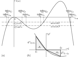
Figure 9: (a) A qualitative shape of the metric functions ${\mathcal{F}}$ and ${\mathcal{G}}$ (in the case ${m\neq 0}$, ${e\neq 0}$) which are polynomials in $\upsilon$ and $\xi$, respectively. It follows from the representation (168) that both functions ${\mathcal{F}}$ and ${\mathcal{G}}$ are, up to the specific rescaling and the constant term, given by the same polynomial ${{\mathrm{S}}(w)}$, the graph of which is presented here. The zeros of ${\mathcal{F}}$ and ${\mathcal{G}}$ are thus given by intersections of the graph of ${\mathrm{S}}$ with the horizontal lines ${-a_{\scriptscriptstyle\Lambda}^{-2}\cosh^{2}\alpha}\,$ and ${-a_{\scriptscriptstyle\Lambda}^{-2}\sinh^{2}\alpha}$, respectively. Relations (17) between the zeros of ${\mathcal{F}}$ and ${\mathcal{G}}$ follows immediately from this fact. (b) A graphical representation of the triangular estimate (173) for the areas ${{\mathcal{A}}_{1},\,{\mathcal{A}}_{2}}$ under the graph of ${\mathcal{G}}^{\prime}$.

First, let us note that ${\mathcal{F}}$ and ${\mathcal{G}}$ can be represented in terms of polynomial ${{\mathrm{S}}(w)}$

$$-\frac{\cosh^{2}\alpha}{a_{\scriptscriptstyle\Lambda}^{2}}\,{\mathcal{F}} ={\mathrm{S}}\Bigl{(}\frac{\cosh\alpha}{a_{\scriptscriptstyle\Lambda}}\,\upsilon\Bigr{)}+\frac{\cosh^{2}\alpha}{a_{\scriptscriptstyle\Lambda}^{2}}{\mbox{\;,}}$$ (168)

$$\frac{\sinh^{2}\alpha}{a_{\scriptscriptstyle\Lambda}^{2}}\,{\mathcal{G}} ={\mathrm{S}}\Bigl{(}\frac{\sinh\alpha}{a_{\scriptscriptstyle\Lambda}}\,\xi\Bigr{)}+\frac{\sinh^{2}\alpha}{a_{\scriptscriptstyle\Lambda}^{2}}{\mbox{\;.}}$$

where

$${\mathrm{S}}(w)=-w^{2}(1-2\,mw+e^{2}w^{2}){\mbox{\;.}}$$ (169)

A typical graph of the polynomial ${{\mathrm{S}}(w)}$ is drawn in Fig. 9. By inspecting the graph we obtain, e.g., relations (17) between the roots of the metric functions ${\mathcal{F}}$ and ${\mathcal{G}}$.

We may also prove some interesting properties, including Eq. (21), of the metric function ${\mathcal{G}}$ in the case of charged accelerated black holes. (Similar properties — in particular the inequality (174) — can be also proved for uncharged accelerated black holes, i.e., for ${e=0}$, ${m\neq 0}$, ${A\neq 0}$.) In the case ${e\neq 0}$, ${A\neq 0}$, the metric function ${\mathcal{G}}$ is a polynomial of the fourth order in $\xi$ and its zeros have been denoted in the ascending order as ${\xi_{1},\,\xi_{2},\,\xi_{3},\,\xi_{4}}$. The extremes of ${\mathcal{G}}$ (zeros of ${\mathcal{G}}^{\prime}$) are ${\xi^{(1)}_{0}=0}$, ${\xi^{(1)}_{\pm}=(3m\pm\sqrt{9m^{2}-8e^{2}})/({4Ae^{2}})}$. The zero of $\,{{\mathcal{G}}^{\prime\prime\prime}=12(Am-2e^{2}A^{2}\xi)}\,$ is $\,{\xi^{(3)}=m/(2Ae^{2})}\,$, and ${{\mathcal{G}}^{\prime\prime\prime}>0}$ for ${\xi<\xi^{(3)}}$. Using the conditions (5), a straightforward calculation leads to an inequality ${{\mathcal{G}}|_{\xi^{(1)}_{+}}>0}$. The condition that ${\mathcal{G}}$ has four real roots requires ${{\mathcal{G}}|_{\xi^{(1)}_{-}}<0}$. This confirms that the graph of ${\mathcal{G}}$ has always a qualitative shape shown on Fig. 9. The extremes of ${\mathcal{G}}$ are located between its zeros, so that ${\xi_{1}<0<\xi_{2}<\xi^{(1)}_{-}}$. Expressing the vanishing linear coefficient in ${\mathcal{G}}$ in terms of the roots we obtain ${(\xi_{1}+\xi_{2})\xi_{3}\xi_{4}=-\xi_{1}\xi_{2}(\xi_{3}+\xi_{4})}$, the right-hand side is clearly positive, as well as ${\xi_{3}\xi_{4}}$, so we obtain

$$-\xi_{1}<\xi_{2}{\mbox{\;.}}$$ (170)

From the conditions (5) it also follows that $\xi^{(1)}_{-}<\xi^{(3)}$ and thus we have

$$\xi_{1}<0<\xi_{2}<\xi^{(1)}_{-}<\xi^{(3)}{\mbox{\;.}}$$ (171)

This means that ${\mathcal{G}}^{\prime}$ is convex on the relevant interval ${(\xi_{1},\xi_{2})}$, it is positive on the interval ${(\xi_{1},0)}$ and negative on ${(0,\xi_{2})}$. The positivity of ${\mathcal{G}}^{\prime\prime\prime}$ on the interval ${(\xi_{1},\xi_{2})}$ also implies ${m-2e^{2}A\,\xi_{\scriptscriptstyle{\boldsymbol{+}}}>0}$, which is the relation used in the discussion following the result (82). Clearly, ${\int_{\xi_{1}}^{\xi_{2}}{\mathcal{G}}^{\prime}d\xi=0}$, i.e., the areas

$${\mathcal{A}}_{1}=\int_{\xi_{1}}^{0}{\mathcal{G}}^{\prime}d\xi{\mbox{\;,\quad}}{\mathcal{A}}_{2}=-\int_{0}^{\xi_{2}}{\mathcal{G}}^{\prime}d\xi$$ (172)

are the same. Thanks to the convexity of ${\mathcal{G}}^{\prime}$, we can estimate ${\mathcal{A}}_{1}$ and ${\mathcal{A}}_{2}$ by simpler triangular areas (see Fig. 9(b)), and we obtain

$$-{\textstyle\frac{1}{2}}\,\xi_{2}\,{\mathcal{G}}^{\prime}|_{\xi=\xi_{2}}<{\mathcal{A}}_{2}={\mathcal{A}}_{1}<-{\textstyle\frac{1}{2}}\,\xi_{1}{\mathcal{G}}^{\prime}|_{\xi=\xi_{1}}{\mbox{\;.}}$$ (173)

Using Eq. (170) this implies

$$-{\mathcal{G}}^{\prime}|_{\xi=\xi_{2}}<{\mathcal{G}}^{\prime}|_{\xi=\xi_{1}}{\mbox{\;.}}$$ (174)

Considering Eq. (20) we obtain the important relation (21) which is necessary for the discussion of conicity in Section III.

Appendix C Relations between the coordinate frames

In this appendix we summarize for convenience the relations between different coordinate 1-form and vector frames

For coordinate 1-form frames ${(\mathbf{d}{\tau},\,\mathbf{d}{\upsilon},\,\mathbf{d}{\xi},\,\mathbf{d}{\varphi})}$, ${(\mathbf{d}{\tau},\,\mathbf{d}{\omega},\,\mathbf{d}{\sigma},\,\mathbf{d}{\varphi})}$, and ${(\mathbf{d}{\zeta},\,\mathbf{d}{\bar{\zeta}},\,\mathbf{d}{r},\,\mathbf{d}{u})}$ we obtain

$$\mathbf{d}\tau =\mathbf{d}\tau =\frac{{\mathcal{E}}}{{\mathcal{F}}\cosh\alpha}\,\frac{1}{a_{\scriptscriptstyle\Lambda}}\,\mathbf{d}u+\frac{1}{{\mathcal{F}}\cosh\alpha}\frac{a_{\scriptscriptstyle\Lambda}}{r^{2}}\,\mathbf{d}r-\frac{{\mathcal{G}}}{{\mathcal{F}}}\tanh\alpha\,\mathbf{d}\psi{\mbox{\;,}}$$ (175a)

$$\mathbf{d}\upsilon =-\frac{{\mathcal{F}}}{{\mathcal{E}}}\,\cosh\alpha\,\mathbf{d}\omega+\frac{{\mathcal{F}}{\mathcal{G}}}{{\mathcal{E}}}\,\sinh\alpha\,\mathbf{d}\sigma =-{\mathcal{G}}\,\frac{\sinh^{2}\alpha}{\cosh\alpha}\,\frac{1}{a_{\scriptscriptstyle\Lambda}}\,\mathbf{d}u-\frac{1}{\cosh\alpha}\frac{a_{\scriptscriptstyle\Lambda}}{r^{2}}\,\mathbf{d}r+{\mathcal{G}}\tanh\alpha\,\mathbf{d}\psi{\mbox{\;,}}$$ (175b)

$$\mathbf{d}\xi =\frac{{\mathcal{G}}}{{\mathcal{E}}}\,\sinh\alpha\,\mathbf{d}\omega+\frac{{\mathcal{F}}{\mathcal{G}}}{{\mathcal{E}}}\,\cosh\alpha\,\mathbf{d}\sigma =-{\mathcal{G}}\sinh\alpha\,\frac{1}{a_{\scriptscriptstyle\Lambda}}\,\mathbf{d}u+{\mathcal{G}}\,\mathbf{d}\psi{\mbox{\;,}}$$ (175c)

$$\mathbf{d}\omega =-\cosh\alpha\,\mathbf{d}\upsilon+\sinh\alpha\,\mathbf{d}\xi =\frac{a_{\scriptscriptstyle\Lambda}}{r^{2}}\,\mathbf{d}r{\mbox{\;,}}$$ (175d)

$$\mathbf{d}\sigma =\frac{\sinh\alpha}{{\mathcal{F}}}\,\mathbf{d}\upsilon+\frac{\cosh\alpha}{{\mathcal{G}}}\,\mathbf{d}\xi =-\frac{{\mathcal{E}}}{{\mathcal{F}}}\,\tanh\alpha\,\frac{1}{a_{\scriptscriptstyle\Lambda}}\,\mathbf{d}u-\frac{\tanh\alpha}{{\mathcal{F}}}\frac{a_{\scriptscriptstyle\Lambda}}{r^{2}}\,\mathbf{d}r+\frac{{\mathcal{E}}}{{\mathcal{F}}\cosh\alpha}\,\mathbf{d}\psi{\mbox{\;,}}$$ (175e)

$$\frac{1}{a_{\scriptscriptstyle\Lambda}}\, \mathbf{d}u =\frac{1}{\cosh\alpha}\,\mathbf{d}\tau+\frac{1}{{\mathcal{F}}\cosh\alpha}\,\mathbf{d}\upsilon =\frac{1}{\cosh\alpha}\,\mathbf{d}\tau-\frac{1}{{\mathcal{E}}}\,\mathbf{d}\omega+\frac{{\mathcal{G}}}{{\mathcal{E}}}\,\tanh\alpha\,\mathbf{d}\sigma{\mbox{\;,}}$$ (175f)

$$\frac{1}{a_{\scriptscriptstyle\Lambda}}\, \mathbf{d}r =-\frac{\cosh\alpha}{\omega^{2}}\,\mathbf{d}\upsilon+\frac{\sinh\alpha}{\omega^{2}}\,\mathbf{d}\xi =\frac{1}{\omega^{2}}\,\mathbf{d}\omega{\mbox{\;,}}$$ (175g)

$$\sqrt{2}\, \mathbf{d}\zeta =\tanh\alpha\,\mathbf{d}\tau+\frac{\tanh\alpha}{{\mathcal{F}}}\,\mathbf{d}\upsilon+\frac{1}{{\mathcal{G}}}\,\mathbf{d}\xi-i\,\mathbf{d}\varphi =\tanh\alpha\,\mathbf{d}\tau+\frac{1}{\cosh\alpha}\,\mathbf{d}\sigma-i\,\mathbf{d}\varphi{\mbox{\;,}}$$ (175h)

where

$$\mathbf{d}\psi=\textstyle\frac{1}{\sqrt{2}}\bigl{(}\mathbf{d}\zeta+\mathbf{d}\bar{\zeta}\bigr{)}{\mbox{\;,\quad}}\mathbf{d}\varphi=\textstyle\frac{i}{\sqrt{2}}\bigl{(}\mathbf{d}\zeta-\mathbf{d}\bar{\zeta}\bigr{)}{\mbox{\;,\quad}}\mathbf{d}\zeta=\textstyle\frac{1}{\sqrt{2}}\bigl{(}\mathbf{d}\psi-i\,\mathbf{d}\varphi\bigr{)}{\mbox{\;,\quad}}\mathbf{d}\bar{\zeta}=\overline{\mathbf{d}\zeta}{\mbox{\;.}}$$ (175i)

Coordinate vector frames ${({{\boldsymbol{\mathbf{\partial}}}_{\tau}},\,{{\boldsymbol{\mathbf{\partial}}}_{\upsilon}},\,{{\boldsymbol{\mathbf{\partial}}}_{\xi}},\,{{\boldsymbol{\mathbf{\partial}}}_{\varphi}})}$, ${({{\boldsymbol{\mathbf{\partial}}}_{\tau}},\,{{\boldsymbol{\mathbf{\partial}}}_{\omega}},\,{{\boldsymbol{\mathbf{\partial}}}_{\sigma}},\,{{\boldsymbol{\mathbf{\partial}}}_{\varphi}})}$, and ${({{\boldsymbol{\mathbf{\partial}}}_{\zeta}},\,{{\boldsymbol{\mathbf{\partial}}}_{\bar{\zeta}}},\,{{\boldsymbol{\mathbf{\partial}}}_{r}},\,{{\boldsymbol{\mathbf{\partial}}}_{u}})}$ are related by

$${{\boldsymbol{\mathbf{\partial}}}_{\tau}} ={{\boldsymbol{\mathbf{\partial}}}_{\tau}} =\frac{1}{\cosh\alpha}\,a_{\scriptscriptstyle\Lambda}\,{{\boldsymbol{\mathbf{\partial}}}_{u}}+\tanh\alpha\,{{\boldsymbol{\mathbf{\partial}}}_{\psi}}{\mbox{\;,}}$$ (176a)

$${{\boldsymbol{\mathbf{\partial}}}_{\upsilon}} =-\cosh\alpha\,{{\boldsymbol{\mathbf{\partial}}}_{\omega}}+\frac{\sinh\alpha}{{\mathcal{F}}}\,{{\boldsymbol{\mathbf{\partial}}}_{\sigma}} =\frac{1}{{\mathcal{F}}\cosh\alpha}\,a_{\scriptscriptstyle\Lambda}\,{{\boldsymbol{\mathbf{\partial}}}_{u}}-\cosh\alpha\,\frac{r^{2}}{a_{\scriptscriptstyle\Lambda}}\,{{\boldsymbol{\mathbf{\partial}}}_{r}}+\frac{\tanh\alpha}{{\mathcal{F}}}\,{{\boldsymbol{\mathbf{\partial}}}_{\psi}}{\mbox{\;,}}$$ (176b)

$${{\boldsymbol{\mathbf{\partial}}}_{\xi}} =\sinh\alpha\,{{\boldsymbol{\mathbf{\partial}}}_{\omega}}+\frac{\cosh\alpha}{{\mathcal{G}}}\,{{\boldsymbol{\mathbf{\partial}}}_{\sigma}} =\sinh\alpha\,\frac{r^{2}}{a_{\scriptscriptstyle\Lambda}}\,{{\boldsymbol{\mathbf{\partial}}}_{r}}+\frac{1}{{\mathcal{G}}}\,{{\boldsymbol{\mathbf{\partial}}}_{\psi}}{\mbox{\;,}}$$ (176c)

$${{\boldsymbol{\mathbf{\partial}}}_{\omega}} =-\frac{{\mathcal{F}}}{{\mathcal{E}}}\,\cosh\alpha\,{{\boldsymbol{\mathbf{\partial}}}_{\upsilon}}+\frac{{\mathcal{G}}}{{\mathcal{E}}}\,\sinh\alpha\,{{\boldsymbol{\mathbf{\partial}}}_{\xi}} =-\frac{1}{{\mathcal{E}}}\,a_{\scriptscriptstyle\Lambda}\,{{\boldsymbol{\mathbf{\partial}}}_{u}}+\frac{r^{2}}{a_{\scriptscriptstyle\Lambda}}\,{{\boldsymbol{\mathbf{\partial}}}_{r}}{\mbox{\;,}}$$ (176d)

$${{\boldsymbol{\mathbf{\partial}}}_{\sigma}} =\frac{{\mathcal{F}}{\mathcal{G}}}{{\mathcal{E}}}\,\sinh\alpha\,{{\boldsymbol{\mathbf{\partial}}}_{\upsilon}}+\frac{{\mathcal{F}}{\mathcal{G}}}{{\mathcal{E}}}\,\cosh\alpha\,{{\boldsymbol{\mathbf{\partial}}}_{\xi}} =\frac{{\mathcal{G}}}{{\mathcal{E}}}\,\tanh\alpha\,a_{\scriptscriptstyle\Lambda}\,{{\boldsymbol{\mathbf{\partial}}}_{u}}+\frac{1}{\cosh\alpha}\,{{\boldsymbol{\mathbf{\partial}}}_{\psi}}{\mbox{\;,}}$$ (176e)

$$a_{\scriptscriptstyle\Lambda}\, {{\boldsymbol{\mathbf{\partial}}}_{u}} =\frac{{\mathcal{E}}}{{\mathcal{F}}\cosh\alpha}\,{{\boldsymbol{\mathbf{\partial}}}_{\tau}}-{\mathcal{G}}\frac{\sinh^{2}\alpha}{\cosh\alpha}\,{{\boldsymbol{\mathbf{\partial}}}_{\upsilon}}-{\mathcal{G}}\sinh\alpha\,{{\boldsymbol{\mathbf{\partial}}}_{\xi}} =\frac{{\mathcal{E}}}{{\mathcal{F}}\cosh\alpha}\,{{\boldsymbol{\mathbf{\partial}}}_{\tau}}-\frac{{\mathcal{E}}}{{\mathcal{F}}}\,\tanh\alpha\,{{\boldsymbol{\mathbf{\partial}}}_{\sigma}}{\mbox{\;,}}$$ (176f)

$$a_{\scriptscriptstyle\Lambda}\, {{\boldsymbol{\mathbf{\partial}}}_{r}} =\frac{\omega^{2}}{{\mathcal{F}}\cosh\alpha}\,{{\boldsymbol{\mathbf{\partial}}}_{\tau}}-\frac{\omega^{2}}{\cosh\alpha}\,{{\boldsymbol{\mathbf{\partial}}}_{\upsilon}} =\frac{\omega^{2}}{{\mathcal{F}}\cosh\alpha}\,{{\boldsymbol{\mathbf{\partial}}}_{\tau}}+\omega^{2}\,{{\boldsymbol{\mathbf{\partial}}}_{\omega}}-\frac{\tanh\alpha}{{\mathcal{F}}}\,\omega^{2}\,{{\boldsymbol{\mathbf{\partial}}}_{\sigma}}{\mbox{\;,}}$$ (176g)

$$\sqrt{2}\, {{\boldsymbol{\mathbf{\partial}}}_{\zeta}} =-\frac{{\mathcal{G}}}{{\mathcal{F}}}\,\tanh\alpha\,{{\boldsymbol{\mathbf{\partial}}}_{\tau}}+{\mathcal{G}}\tanh\alpha\,{{\boldsymbol{\mathbf{\partial}}}_{\upsilon}}+{\mathcal{G}}{{\boldsymbol{\mathbf{\partial}}}_{\xi}}+i\,{{\boldsymbol{\mathbf{\partial}}}_{\varphi}} =-\frac{{\mathcal{G}}}{{\mathcal{F}}}\,\tanh\alpha\,{{\boldsymbol{\mathbf{\partial}}}_{\tau}}+\frac{{\mathcal{E}}}{{\mathcal{F}}\cosh\alpha}\,{{\boldsymbol{\mathbf{\partial}}}_{\sigma}}+i\,{{\boldsymbol{\mathbf{\partial}}}_{\varphi}}{\mbox{\;,}}$$ (176h)

where

$${{\boldsymbol{\mathbf{\partial}}}_{\psi}}=\textstyle\frac{1}{\sqrt{2}}\bigl{(}{{\boldsymbol{\mathbf{\partial}}}_{\zeta}}+{{\boldsymbol{\mathbf{\partial}}}_{\bar{\zeta}}}\bigr{)}{\mbox{\;,\quad}}{{\boldsymbol{\mathbf{\partial}}}_{\varphi}}=-\textstyle\frac{i}{\sqrt{2}}\bigl{(}{{\boldsymbol{\mathbf{\partial}}}_{\zeta}}-{{\boldsymbol{\mathbf{\partial}}}_{\bar{\zeta}}}\bigr{)}{\mbox{\;,\quad}}{{\boldsymbol{\mathbf{\partial}}}_{\zeta}}=\textstyle\frac{1}{\sqrt{2}}\bigl{(}{{\boldsymbol{\mathbf{\partial}}}_{\psi}}+i\,{{\boldsymbol{\mathbf{\partial}}}_{\varphi}}\bigr{)}{\mbox{\;,\quad}}{{\boldsymbol{\mathbf{\partial}}}_{\bar{\zeta}}}=\overline{{{\boldsymbol{\mathbf{\partial}}}_{\zeta}}}{\mbox{\;.}}$$ (176i)

It is also useful to express the relations between different null tetrads introduced in the paper. The special null tetrad (defined by Eq. (29), using Eq. (23)) the reference null tetrad (see Eq. (35)), and the Robinson-Trautman tetrad (56) are related by

$${{\boldsymbol{\mathbf{k}}}}_{\mathrm{s}} =\frac{1}{2}\tan\theta_{\mathrm{s}}\,\Bigl{(}\cot\frac{\theta_{\mathrm{s}}}{2}\;{{\boldsymbol{\mathbf{k}}}}_{\mathrm{o}}+\tan\frac{\theta_{\mathrm{s}}}{2}\;{{\boldsymbol{\mathbf{l}}}}_{\mathrm{o}}+{{\boldsymbol{\mathbf{m}}}}_{\mathrm{o}}+{\bar{{\boldsymbol{\mathbf{m}}}}}_{\mathrm{o}}\Bigr{)} {\mspace{-20.0mu}}=\exp(-\beta_{\scriptscriptstyle\mathrm{RT}})\sec{\theta_{\mathrm{s}}}\,{{\boldsymbol{\mathbf{k}}}}_{\scriptscriptstyle\mathrm{RT}}{\mbox{\;,}}$$

$${{\boldsymbol{\mathbf{l}}}}_{\mathrm{s}} =\frac{1}{2}\tan\theta_{\mathrm{s}}\,\Bigl{(}\tan\frac{\theta_{\mathrm{s}}}{2}\;{{\boldsymbol{\mathbf{k}}}}_{\mathrm{o}}+\cot\frac{\theta_{\mathrm{s}}}{2}\;{{\boldsymbol{\mathbf{l}}}}_{\mathrm{o}}+{{\boldsymbol{\mathbf{m}}}}_{\mathrm{o}}+{\bar{{\boldsymbol{\mathbf{m}}}}}_{\mathrm{o}}\Bigr{)} {\mspace{-20.0mu}}=\sin\theta_{\mathrm{s}}\,\Bigl{(}\exp(-\beta_{\scriptscriptstyle\mathrm{RT}})\tan\theta_{\mathrm{s}}\,{{\boldsymbol{\mathbf{k}}}}_{\scriptscriptstyle\mathrm{RT}}+\exp(\beta_{\scriptscriptstyle\mathrm{RT}})\cot\theta_{\mathrm{s}}\,{{\boldsymbol{\mathbf{l}}}}_{\scriptscriptstyle\mathrm{RT}}+{{\boldsymbol{\mathbf{m}}}}_{\scriptscriptstyle\mathrm{RT}}+{\bar{{\boldsymbol{\mathbf{m}}}}}_{\scriptscriptstyle\mathrm{RT}}\Bigr{)}{\mbox{\;,}}$$

$${{\boldsymbol{\mathbf{m}}}}_{\mathrm{s}} =\frac{1}{2}\tan\theta_{\mathrm{s}}\,\Bigl{(}{{\boldsymbol{\mathbf{k}}}}_{\mathrm{o}}+{{\boldsymbol{\mathbf{l}}}}_{\mathrm{o}}+\cot\frac{\theta_{\mathrm{s}}}{2}\;{{\boldsymbol{\mathbf{m}}}}_{\mathrm{o}}+\tan\frac{\theta_{\mathrm{s}}}{2}\;{\bar{{\boldsymbol{\mathbf{m}}}}}_{\mathrm{o}}\Bigr{)} {\mspace{-20.0mu}}={{\boldsymbol{\mathbf{m}}}}_{\scriptscriptstyle\mathrm{RT}}+\exp(-\beta_{\scriptscriptstyle\mathrm{RT}})\tan\theta_{\mathrm{s}}\,{{\boldsymbol{\mathbf{k}}}}_{\scriptscriptstyle\mathrm{RT}}{\mbox{\;,}}$$ (177)

$${\bar{{\boldsymbol{\mathbf{m}}}}}_{\mathrm{s}} =\frac{1}{2}\tan\theta_{\mathrm{s}}\,\Bigl{(}{{\boldsymbol{\mathbf{k}}}}_{\mathrm{o}}+{{\boldsymbol{\mathbf{l}}}}_{\mathrm{o}}+\tan\frac{\theta_{\mathrm{s}}}{2}\;{{\boldsymbol{\mathbf{m}}}}_{\mathrm{o}}+\cot\frac{\theta_{\mathrm{s}}}{2}\;{\bar{{\boldsymbol{\mathbf{m}}}}}_{\mathrm{o}}\Bigr{)} {\mspace{-20.0mu}}={\bar{{\boldsymbol{\mathbf{m}}}}}_{\scriptscriptstyle\mathrm{RT}}+\exp(-\beta_{\scriptscriptstyle\mathrm{RT}})\tan\theta_{\mathrm{s}}\,{{\boldsymbol{\mathbf{k}}}}_{\scriptscriptstyle\mathrm{RT}}{\mbox{\;,}}$$

$${{\boldsymbol{\mathbf{k}}}}_{\scriptscriptstyle\mathrm{RT}} =\frac{1}{2}\exp({\mspace{14.5mu}}\beta_{\scriptscriptstyle\mathrm{RT}})\sin\theta_{\mathrm{s}}\,\Bigl{(}\cot\frac{\theta_{\mathrm{s}}}{2}\,{{\boldsymbol{\mathbf{k}}}}_{\mathrm{o}}+\tan\frac{\theta_{\mathrm{s}}}{2}\,{{\boldsymbol{\mathbf{l}}}}_{\mathrm{o}}+{{\boldsymbol{\mathbf{m}}}}_{\mathrm{o}}+{\bar{{\boldsymbol{\mathbf{m}}}}}_{\mathrm{o}}\Bigr{)} {\mspace{-20.0mu}}=\exp(\beta_{\scriptscriptstyle\mathrm{RT}})\cos\theta_{\mathrm{s}}\,{{\boldsymbol{\mathbf{k}}}}_{\mathrm{s}}{\mbox{\;,}}$$

$${{\boldsymbol{\mathbf{l}}}}_{\scriptscriptstyle\mathrm{RT}} =\frac{1}{2}\exp(-\beta_{\scriptscriptstyle\mathrm{RT}})\sin\theta_{\mathrm{s}}\,\Bigl{(}\tan\frac{\theta_{\mathrm{s}}}{2}\,{{\boldsymbol{\mathbf{k}}}}_{\mathrm{o}}+\cot\frac{\theta_{\mathrm{s}}}{2}\,{{\boldsymbol{\mathbf{l}}}}_{\mathrm{o}}-{{\boldsymbol{\mathbf{m}}}}_{\mathrm{o}}-{\bar{{\boldsymbol{\mathbf{m}}}}}_{\mathrm{o}}\Bigr{)} {\mspace{-20.0mu}}=\exp(-\beta_{\scriptscriptstyle\mathrm{RT}})\tan\theta_{\mathrm{s}}\,\Bigl{(}\sin\theta_{\mathrm{s}}\,{{\boldsymbol{\mathbf{k}}}}_{\mathrm{s}}+\csc\theta_{\mathrm{s}}\,{{\boldsymbol{\mathbf{l}}}}_{\mathrm{s}}-{{\boldsymbol{\mathbf{m}}}}_{\mathrm{s}}-{\bar{{\boldsymbol{\mathbf{m}}}}}_{\mathrm{s}}\Bigr{)}{\mbox{\;,}}$$

$${{\boldsymbol{\mathbf{m}}}}_{\scriptscriptstyle\mathrm{RT}} =\frac{1}{2}\sin\theta_{\mathrm{s}}\,\Bigl{(}-{{\boldsymbol{\mathbf{k}}}}_{\mathrm{o}}+{{\boldsymbol{\mathbf{l}}}}_{\mathrm{o}}+\cot\frac{\theta_{\mathrm{s}}}{2}\,{{\boldsymbol{\mathbf{m}}}}_{\mathrm{o}}-\tan\frac{\theta_{\mathrm{s}}}{2}\,{\bar{{\boldsymbol{\mathbf{m}}}}}_{\mathrm{o}}\Bigr{)} {\mspace{-20.0mu}}={{\boldsymbol{\mathbf{m}}}}_{\mathrm{s}}-\sin\theta_{\mathrm{s}}\,{{\boldsymbol{\mathbf{k}}}}_{\mathrm{s}}{\mbox{\;,}}$$ (178)

$${\bar{{\boldsymbol{\mathbf{m}}}}}_{\scriptscriptstyle\mathrm{RT}} =\frac{1}{2}\sin\theta_{\mathrm{s}}\,\Bigl{(}-{{\boldsymbol{\mathbf{k}}}}_{\mathrm{o}}+{{\boldsymbol{\mathbf{l}}}}_{\mathrm{o}}-\tan\frac{\theta_{\mathrm{s}}}{2}\,{{\boldsymbol{\mathbf{m}}}}_{\mathrm{o}}+\cot\frac{\theta_{\mathrm{s}}}{2}\,{\bar{{\boldsymbol{\mathbf{m}}}}}_{\mathrm{o}}\Bigr{)} {\mspace{-20.0mu}}={\bar{{\boldsymbol{\mathbf{m}}}}}_{\mathrm{s}}-\sin\theta_{\mathrm{s}}\,{{\boldsymbol{\mathbf{k}}}}_{\mathrm{s}}{\mbox{\;.}}$$

The factor $\beta_{\scriptscriptstyle\mathrm{RT}}$ is defined in Eq. (58). The rotated null tetrad (cf.  Eq. (54)) is related to the reference tetrad as

$${{\boldsymbol{\mathbf{k}}}}_{\mathrm{r}} =\frac{1}{2}\sin\theta\,\Bigl{(}\cot{\frac{\theta}{2}}\;{{\boldsymbol{\mathbf{k}}}}_{\mathrm{o}}+\tan{\frac{\theta}{2}}\;{{\boldsymbol{\mathbf{l}}}}_{\mathrm{o}}+\exp(i\phi)\,{{\boldsymbol{\mathbf{m}}}}_{\mathrm{o}}+\exp(-i\phi)\,{\bar{{\boldsymbol{\mathbf{m}}}}}_{\mathrm{o}}\Bigr{)}{\mbox{\;,}}\mspace{340.0mu}$$ (179)

$${{\boldsymbol{\mathbf{l}}}}_{\mathrm{r}} =\frac{1}{2}\sin\theta\,\Bigl{(}\tan{\frac{\theta}{2}}\;{{\boldsymbol{\mathbf{k}}}}_{\mathrm{o}}+\cot{\frac{\theta}{2}}\;{{\boldsymbol{\mathbf{l}}}}_{\mathrm{o}}-\exp(i\phi)\,{{\boldsymbol{\mathbf{m}}}}_{\mathrm{o}}-\exp(-i\phi)\,{\bar{{\boldsymbol{\mathbf{m}}}}}_{\mathrm{o}}\Bigr{)}{\mbox{\;,}}$$

$${{\boldsymbol{\mathbf{m}}}}_{\mathrm{r}} =\frac{1}{2}\sin\theta\,\Bigl{(}-{{\boldsymbol{\mathbf{k}}}}_{\mathrm{o}}+{{\boldsymbol{\mathbf{l}}}}_{\mathrm{o}}+\cot{\frac{\theta}{2}}\,\exp(i\phi)\,{{\boldsymbol{\mathbf{m}}}}_{\mathrm{o}}-\tan{\frac{\theta}{2}}\,\exp(-i\phi)\,{\bar{{\boldsymbol{\mathbf{m}}}}}_{\mathrm{o}}\Bigr{)}{\mbox{\;,}}$$

$${\bar{{\boldsymbol{\mathbf{m}}}}}_{\mathrm{r}} =\frac{1}{2}\sin\theta\,\Bigl{(}-{{\boldsymbol{\mathbf{k}}}}_{\mathrm{o}}+{{\boldsymbol{\mathbf{l}}}}_{\mathrm{o}}-\tan{\frac{\theta}{2}}\,\exp(i\phi)\,{{\boldsymbol{\mathbf{m}}}}_{\mathrm{o}}+\cot{\frac{\theta}{2}}\,\exp(-i\phi)\,{\bar{{\boldsymbol{\mathbf{m}}}}}_{\mathrm{o}}\Bigr{)}{\mbox{\;.}}$$

Here, the angle $\theta_{\mathrm{s}}$ is defined by Eq. (40).

Appendix D Transformations of the components $\Psi_{n}$ and $\Phi_{n}$

The components $\Psi_{n}$ of the Weyl tensor (see note nt:WTcomp ),

$$\begin{gathered}\Psi_{0}={\boldsymbol{\mathbf{C}}}_{\kappa\mu\kappa\mu}{\mbox{\;,\quad}}\Psi_{4}={\boldsymbol{\mathbf{C}}}_{\lambda{\bar{\mu}}\lambda{\bar{\mu}}}{\mbox{\;,}}\\ \Psi_{1}=-{\boldsymbol{\mathbf{C}}}_{\kappa\mu\mu{\bar{\mu}}}=-{\boldsymbol{\mathbf{C}}}_{\mu{\bar{\mu}}\kappa\mu}={\boldsymbol{\mathbf{C}}}_{\kappa\lambda\kappa\mu}={\boldsymbol{\mathbf{C}}}_{\kappa\mu\kappa\lambda}{\mbox{\;,}}\\ \Psi_{3}=-{\boldsymbol{\mathbf{C}}}_{\kappa\lambda\lambda{\bar{\mu}}}=-{\boldsymbol{\mathbf{C}}}_{\lambda{\bar{\mu}}\kappa\lambda}={\boldsymbol{\mathbf{C}}}_{\lambda{\bar{\mu}}\mu{\bar{\mu}}}={\boldsymbol{\mathbf{C}}}_{\mu{\bar{\mu}}\lambda{\bar{\mu}}}{\mbox{\;,}}\\ \Psi_{2}=-{\boldsymbol{\mathbf{C}}}_{\kappa\mu\lambda{\bar{\mu}}}=-{\boldsymbol{\mathbf{C}}}_{\lambda{\bar{\mu}}\kappa\mu}{\mbox{\;,}}\\ 2\operatorname{Re}\Psi_{2}={\boldsymbol{\mathbf{C}}}_{\kappa\lambda\kappa\lambda}={\boldsymbol{\mathbf{C}}}_{\mu{\bar{\mu}}\mu{\bar{\mu}}}{\mbox{\;,}}\\ 2\operatorname{Im}\Psi_{2}=i\,{\boldsymbol{\mathbf{C}}}_{\kappa\lambda\mu{\bar{\mu}}}=i\,{\boldsymbol{\mathbf{C}}}_{\mu{\bar{\mu}}\kappa\lambda}{\mbox{\;,}}\end{gathered}$$ (180)

and the components $\Phi_{n}$ of tensor of electromagnetic field

$$\Phi_{0} ={\boldsymbol{\mathbf{F}}}_{\kappa\mu}{\mbox{\;,}} 2\operatorname{Re}\Phi_{1} ={\boldsymbol{\mathbf{F}}}_{\kappa\lambda}{\mbox{\;,}}$$ (181)

$$\Phi_{2} ={\boldsymbol{\mathbf{F}}}_{{\bar{\mu}}\lambda}{\mbox{\;,}} 2\operatorname{Im}\Phi_{1} =i\,{\boldsymbol{\mathbf{F}}}_{\mu{\bar{\mu}}}{\mbox{\;,}}$$

transform in the well-known way under special Lorentz transformations, see, e.g., Ref. Kramer et al. (1980).

For a null rotation with ${{\boldsymbol{\mathbf{k}}}}$ fixed,

$${{\boldsymbol{\mathbf{k}}}} ={{\boldsymbol{\mathbf{k}}}}_{\mathrm{o}}{\mbox{\;,}}$$ (182)

$${{\boldsymbol{\mathbf{l}}}} ={{\boldsymbol{\mathbf{l}}}}_{\mathrm{o}}+\bar{L}{{\boldsymbol{\mathbf{m}}}}_{\mathrm{o}}+L{\bar{{\boldsymbol{\mathbf{m}}}}}_{\mathrm{o}}+L\bar{L}{{\boldsymbol{\mathbf{k}}}}_{\mathrm{o}}{\mbox{\;,}}$$

$${{\boldsymbol{\mathbf{m}}}} ={{\boldsymbol{\mathbf{m}}}}_{\mathrm{o}}+L{{\boldsymbol{\mathbf{k}}}}_{\mathrm{o}}{\mbox{\;,}}$$

$${\bar{{\boldsymbol{\mathbf{m}}}}} ={\bar{{\boldsymbol{\mathbf{m}}}}}_{\mathrm{o}}+\bar{L}{{\boldsymbol{\mathbf{k}}}}_{\mathrm{o}}{\mbox{\;,}}$$

$L$ being a complex number which parametrize the rotation, the components of the Weyl tensor transform as

$$\begin{split}\Psi_{0}&=\Psi^{{\mathrm{o}}}_{0}{\mbox{\;,}}\\ \Psi_{1}&={\bar{L}}\,\Psi^{{\mathrm{o}}}_{0}+\Psi^{{\mathrm{o}}}_{1}{\mbox{\;,}}\\ \Psi_{2}&={\bar{L}}^{2}\Psi^{{\mathrm{o}}}_{0}+2{\bar{L}}\,\Psi^{{\mathrm{o}}}_{1}+\Psi^{{\mathrm{o}}}_{2}{\mbox{\;,}}\\ \Psi_{3}&={\bar{L}}^{3}\Psi^{{\mathrm{o}}}_{0}+3{\bar{L}}^{2}\Psi^{{\mathrm{o}}}_{1}+3{\bar{L}}\,\Psi^{{\mathrm{o}}}_{2}+\Psi^{{\mathrm{o}}}_{3}{\mbox{\;,}}\\ \Psi_{4}&={\bar{L}}^{4}\Psi^{{\mathrm{o}}}_{0}+4{\bar{L}}^{3}\Psi^{{\mathrm{o}}}_{1}+6{\bar{L}}^{2}\Psi^{{\mathrm{o}}}_{2}+4{\bar{L}}\,\Psi^{{\mathrm{o}}}_{3}+\Psi^{{\mathrm{o}}}_{4}{\mbox{\;,}}\end{split}$$ (183)

and the components of tensor of electromagnetic field transform according to

$$\Phi_{0} =\Phi^{{\mathrm{o}}}_{0}{\mbox{\;,}}$$ (184)

$$\Phi_{1} ={\bar{L}}\,\Phi^{{\mathrm{o}}}_{0}+\Phi^{{\mathrm{o}}}_{1}{\mbox{\;,}}$$

$$\Phi_{2} ={\bar{L}}^{2}\Phi^{{\mathrm{o}}}_{0}+2{\bar{L}}\,\Phi^{{\mathrm{o}}}_{1}+\Phi^{{\mathrm{o}}}_{2}{\mbox{\;.}}$$

Under a null rotation with ${{\boldsymbol{\mathbf{l}}}}$ fixed,

$${{\boldsymbol{\mathbf{k}}}} ={{\boldsymbol{\mathbf{k}}}}_{\mathrm{o}}+\bar{K}{{\boldsymbol{\mathbf{m}}}}_{\mathrm{o}}+K{\bar{{\boldsymbol{\mathbf{m}}}}}_{\mathrm{o}}+K\bar{K}{{\boldsymbol{\mathbf{l}}}}_{\mathrm{o}}{\mbox{\;,}}$$ (185)

$${{\boldsymbol{\mathbf{l}}}} ={{\boldsymbol{\mathbf{l}}}}_{\mathrm{o}}{\mbox{\;,}}$$

$${{\boldsymbol{\mathbf{m}}}} ={{\boldsymbol{\mathbf{m}}}}_{\mathrm{o}}+K{{\boldsymbol{\mathbf{l}}}}_{\mathrm{o}}{\mbox{\;,}}$$

$${\bar{{\boldsymbol{\mathbf{m}}}}} ={\bar{{\boldsymbol{\mathbf{m}}}}}_{\mathrm{o}}+\bar{K}{{\boldsymbol{\mathbf{l}}}}_{\mathrm{o}}{\mbox{\;,}}$$

$K$ being a complex number which parametrize the rotation, the components of the Weyl tensor transform as

$$\begin{split}\Psi_{0}&=K^{4}\Psi^{{\mathrm{o}}}_{4}+4K^{3}\Psi^{{\mathrm{o}}}_{3}+6K^{2}\Psi^{{\mathrm{o}}}_{2}+4K\,\Psi^{{\mathrm{o}}}_{1}+\Psi^{{\mathrm{o}}}_{0}{\mbox{\;,}}\\ \Psi_{1}&=K^{3}\Psi^{{\mathrm{o}}}_{4}+3K^{2}\Psi^{{\mathrm{o}}}_{3}+3K\,\Psi^{{\mathrm{o}}}_{2}+\Psi^{{\mathrm{o}}}_{1}{\mbox{\;,}}\\ \Psi_{2}&=K^{2}\Psi^{{\mathrm{o}}}_{4}+2K\,\Psi^{{\mathrm{o}}}_{3}+\Psi^{{\mathrm{o}}}_{2}{\mbox{\;,}}\\ \Psi_{3}&=K\,\Psi^{{\mathrm{o}}}_{4}+\Psi^{{\mathrm{o}}}_{3}{\mbox{\;,}}\\ \Psi_{4}&=\Psi^{{\mathrm{o}}}_{4}{\mbox{\;,}}\end{split}$$ (186)

and for electromagnetic field we have

$$\Phi_{0} =K^{2}\Phi^{{\mathrm{o}}}_{2}+2K\,\Phi^{{\mathrm{o}}}_{1}+\Phi^{{\mathrm{o}}}_{0}{\mbox{\;,}}$$ (187)

$$\Phi_{1} =K\,\Phi^{{\mathrm{o}}}_{2}+\Phi^{{\mathrm{o}}}_{1}{\mbox{\;,}}$$

$$\Phi_{2} =\Phi^{{\mathrm{o}}}_{2}{\mbox{\;.}}$$

A boost in the ${{{\boldsymbol{\mathbf{n}}}}{\text{-}}{{\boldsymbol{\mathbf{q}}}}\equiv{{\boldsymbol{\mathbf{k}}}}{\text{-}}{{\boldsymbol{\mathbf{l}}}}}$ plane and a spatial rotation in the ${{{\boldsymbol{\mathbf{r}}}}{\text{-}}{{\boldsymbol{\mathbf{s}}}}\equiv{{\boldsymbol{\mathbf{m}}}}{\text{-}}{\bar{{\boldsymbol{\mathbf{m}}}}}}$ plane is given by

$$\begin{gathered}{{\boldsymbol{\mathbf{k}}}}=B\,{{\boldsymbol{\mathbf{k}}}}_{\mathrm{o}}{\mbox{\;,\quad}}{{\boldsymbol{\mathbf{l}}}}=B^{-1}\,{{\boldsymbol{\mathbf{l}}}}_{\mathrm{o}}{\mbox{\;,}}\\ {{\boldsymbol{\mathbf{m}}}}=\exp(i\Phi)\,{{\boldsymbol{\mathbf{m}}}}_{\mathrm{o}}{\mbox{\;,\quad}}{\bar{{\boldsymbol{\mathbf{m}}}}}=\exp(-i\Phi)\,{\bar{{\boldsymbol{\mathbf{m}}}}}_{\mathrm{o}}{\mbox{\;,}}\end{gathered}$$ (188)

or, introducing ${B=\exp\beta}$,

$${{\boldsymbol{\mathbf{n}}}} =\cosh\beta\,{{\boldsymbol{\mathbf{n}}}}_{\mathrm{o}}+\sinh\beta\,{{\boldsymbol{\mathbf{q}}}}_{\mathrm{o}}{\mbox{\;,}}$$ (189)

$${{\boldsymbol{\mathbf{q}}}} =\sinh\beta\,{{\boldsymbol{\mathbf{n}}}}_{\mathrm{o}}+\cosh\beta\,{{\boldsymbol{\mathbf{q}}}}_{\mathrm{o}}{\mbox{\;,}}$$

$${{\boldsymbol{\mathbf{r}}}} ={\mspace{14.5mu}}\cos\Phi\,{{\boldsymbol{\mathbf{r}}}}_{\mathrm{o}}+\sin\Phi\,{{\boldsymbol{\mathbf{s}}}}_{\mathrm{o}}{\mbox{\;,}}$$

$${{\boldsymbol{\mathbf{s}}}} =-\sin\Phi\,{{\boldsymbol{\mathbf{r}}}}_{\mathrm{o}}+\cos\Phi\,{{\boldsymbol{\mathbf{s}}}}_{\mathrm{o}}{\mbox{\;,}}$$

$B$, $\beta$ being real numbers which parametrize the boost, $\Phi$ parametrizing an angle of the rotation. The components $\Psi_{n}$ now transform

$$\Psi_{0} =B^{2}\,\exp(2i\Phi)\;\Psi^{{\mathrm{o}}}_{0}{\mbox{\;,}}$$

$$\Psi_{1} =B\;\;\exp(i\Phi)\;\Psi^{{\mathrm{o}}}_{1}{\mbox{\;,}}$$

$$\Psi_{2} =\Psi^{{\mathrm{o}}}_{2}{\mbox{\;,}}$$ (190)

$$\Psi_{3} =B^{-1}\;\exp(-i\Phi)\;\Psi^{{\mathrm{o}}}_{3}{\mbox{\;,}}$$

$$\Psi_{4} =B^{-2}\,\exp(-2i\Phi)\;\Psi^{{\mathrm{o}}}_{4}{\mbox{\;,}}$$

and $\Phi_{n}$ transform as

$$\Phi_{0} =B\;\;\exp(i\Phi)\;\Phi^{{\mathrm{o}}}_{0}{\mbox{\;,}}$$

$$\Phi_{1} =\Phi^{{\mathrm{o}}}_{1}{\mbox{\;,}}$$ (191)

$$\Phi_{2} =B^{-1}\,\exp(-i\Phi)\;\Phi^{{\mathrm{o}}}_{2}{\mbox{\;.}}$$

References

Bondi (1960)
H. Bondi,
Nature 186,
535 (1960).
Bondi et al. (1962)
H. Bondi,
M. G. J. van der Burg,
and A. W. K.
Metzner, Proc. R. Soc. Lond., Ser A
269, 21 (1962).
Sachs (1962)
R. K. Sachs,
Proc. R. Soc. Lond., Ser A 270,
103 (1962).
van der Burg (1969)
M. G. J. van der Burg,
Proc. R. Soc. Lond., Ser A 310,
221 (1969).
Newman and Penrose (1962)
E. Newman and
R. Penrose,
J. Math. Phys. 3,
566 (1962).
Newman and Unti (1962)
E. T. Newman and
T. W. J. Unti,
J. Math. Phys. 3,
891 (1962).
Sachs (1961)
R. Sachs,
Proc. R. Soc. Lond., Ser A 264,
309 (1961).
Penrose (1965)
R. Penrose,
Proc. R. Soc. Lond., Ser A 284,
159 (1965).
Penrose (1964)
R. Penrose, in
Relativity, Groups and Topology, Les Houches
1963, edited by C. DeWitt
and B. DeWitt
(Gordon and Breach, New York,
1964).
Penrose (1967)
R. Penrose, in
The Nature of Time, edited by
T. Gold
(Cornell University Press, Ithaca, New
York, 1967), pp. 42–54.
Penrose (1963)
R. Penrose,
Phys. Rev. Lett. 10,
66 (1963).
Bondi et al. (1959)
H. Bondi,
F. A. E. Pirani,
and I. Robinson,
Proc. R. Soc. Lond., Ser A 251,
519 (1959).
Ehlers and Kundt (1962)
J. Ehlers and
W. Kundt, in
Gravitation: an Introduction to Current Research,
edited by L. Witten
(John Wiley, New York,
1962), pp. 49–101.
Robinson and Trautman (1962)
I. Robinson and
A. Trautman,
Proc. R. Soc. Lond., Ser A 265,
463 (1962).
Bonnor and
Swaminarayan (1964)
W. B. Bonnor and
N. S. Swaminarayan,
Z. Phys. 177,
240 (1964).
Pirani (1965)
F. A. E. Pirani, in
Brandeis Lectures on General Relativity, edited
by S. Deser and
K. W. Ford
(Prentice-Hall, New Jersey,
1965), pp. 249–372.
Bonnor et al. (1994)
W. B. Bonnor,
J. B. Griffiths,
and M. A. H.
MacCallum, Gen. Rel. Grav.
26, 687 (1994).
Bičák (1985)
J. Bičák, in
Galaxies, Axisymmetric Systems and Relativity,
edited by M. A. H. MacCaluum
(Cambridge University Press,
Cambridge, 1985), pp.
91–124.
Bičák (1997)
J. Bičák, in
Relativistic Gravitation and Gravitational
Radiation, Les Louches 1995, edited by
J.-A. Marck and
J.-P. Lasota
(Cambridge University Press,
Cambridge, 1997), pp.
67–87.
Bičák (2000)
J. Bičák, in
Einstein’s Field Equations and Their Physical
Implications, edited by B. G.
Schmidt (Springer,
Berlin, 2000), vol. 540,
pp. 1–126, eprint gr-qc/0004016.
Bičák and Krtouš (2001)
J. Bičák
and
P. Krtouš,
Phys. Rev. D 64,
124020 (2001), eprint gr-qc/0107078.
Bičák and
Krtouš (2002)
J. Bičák
and
P. Krtouš,
Phys. Rev. Lett. 88,
211101 (2002), eprint gr-qc/0207010.
(23)
J. Bičák
and
P. Krtouš,
unpublished.
Bičák and Schmidt (1989)
J. Bičák
and B. G.
Schmidt, Phys. Rev. D
40, 1827 (1989).
Levi-Civita (1917)
T. Levi-Civita,
Rend. Acc. Lincei 26,
307 (1917).
Weyl (1918)
H. Weyl, Ann.
Phys. (Leipzig) 59, 185
(1918).
Kinnersley and Walker (1970)
W. Kinnersley and
M. Walker,
Phys. Rev. D 2,
1359 (1970).
Bonnor (1983)
W. B. Bonnor,
Gen. Rel. Grav. 15,
535 (1983).
Bičák and Pravda (1999)
J. Bičák
and V. Pravda,
Phys. Rev. D 60,
044004 (1999).
Letelier and Oliveira (2001)
P. S. Letelier and
S. R. Oliveira,
Phys. Rev. D 64,
064005 (2001), eprint gr-qc/9809089.
Pravda and Pravdová (2000)
V. Pravda and
A. Pravdová,
Czech. J. Phys. 50,
333 (2000).
Plebański and
Demiański (1976)
J. Plebański
and
M. Demiański,
Ann. Phys. (N.Y.) 98,
98 (1976).
Carter (1968)
B. Carter,
Commun. Math. Phys. 10,
280 (1968).
Mann and Ross (1995)
R. B. Mann and
S. F. Ross,
Phys. Rev. D 52,
2254 (1995).
Podolský and
Griffiths (2001)
J. Podolský
and J. B.
Griffiths, Phys. Rev. D
63, 024006
(2001), eprint gr-qc/0010109.
Dias and Lemos (a)
O. J. C. Dias and
J. P. S. Lemos, Phys. Rev. D
67, 064001
(2003), eprint hep-th/0210065.
Dias and Lemos (b)
O. J. C. Dias and
J. P. S. Lemos, Phys. Rev. D
67, 084018
(2003), eprint hep-th/0301046.
(39)
We use here the unit conventions of Ref. Misner et al. (1973)
(which is somewhat different from Ref. Kramer et al. (1980)), namely,
we assume “geometrical” values of the gravitational constant
, and of the electric permittivity .
These constants are fixed by the Einstein equation ,
and the Maxwell equation .
Both the mass and the charge thus have the dimension of length.
The constants , can be explicitly reinserted into the expressions using
a dimensional analysis with the help of relations ,
and .
For example, , with the mass
measured in and the charge in .
Note, however, that because the tensor of electromagnetic field is not dimensionless,
we, in fact, obtain .
(Of course, is always assumed here.)
Misner et al. (1973)
C. W. Misner,
K. S. Thorne,
and J. A.
Wheeler, Gravitation
(Freeman, San Francisco,
1973).
(41)
A symmetric product of two 1-forms is defined as
For example, the metric (14) written in a more common (but less precise) notation would
read
Penrose and Rindler (1984)
R. Penrose and
W. Rindler,
Spinors and Space-time (Cambridge
University Press, Cambridge, 1984).
Vilenkin and Shellard (1994)
A. Vilenkin and
E. P. S. Shellard,
Cosmic Strings and other Topological Defects
(Cambridge University Press,
Cambridge, 1994).
Kramer et al. (1980)
D. Kramer,
H. Stephani,
E. Herlt, and
M. MacCallum,
Exact Solutions of Einstein’s Field Equation
(Cambridge University Press,
Cambridge, 1980).
(45)
The 4-momentum of the ray is
a tangent vector with respect to a physical dimensionless
affine parameter . Since we are not interested
in dynamical properties of the rays but rather in
behavior of fields at “large distances”, we are using the
affine parameter which has the dimension of length. The
relation between this “distance” parameter
and the physical parameter which determines energy
can conventionally be chosen as .
Therefore, .
(46)
We cannot define here “the same proximity to ”
using some fixed value of the affine parameter , since we wish to use
this procedure to determine the specific normalization of the affine parameter.
(47)
A general choice of final conditions
at infinity might cause a degenerated values of the vector
in finite domains of the spacetime.
(48)
In fact, Ref. Bičák and
Krtouš (2002) use a different notation for
quantities defined in the present paper. When comparing the angular
dependence of Eq. (15) of Ref. Bičák and
Krtouš (2002) with
Eq. (86) it is necessary to use the following dictionary:
,
,
,
, and
In the case , we can also identify
and express of Ref. Bičák and
Krtouš (2002) in
terms of and . The normalization of Eq. (86) and of
the result of Ref. Bičák and
Krtouš (2002) does not coincide due to different
choice of initial conditions for the interpretation tetrads here and in
Ref. Bičák and
Krtouš (2002) (cf. Section VII). Let us also
note that Ref. Bičák and
Krtouš (2002) uses the unit convention in
the sense of note nt:Units instead of here.
(49)
This method has been used in Ref. Bičák and
Krtouš (2002).
Deser and Levin (1999)
S. Deser and
O. Levin,
Phys. Rev. D 59,
064004 (1999).
(51)
P. Krtouš,
J. Podolský,
and
J. Bičák,
in preparation.
Podolský (2002)
J. Podolský,
Czech. J. Phys. 52,
1 (2002), eprint gr-qc/0202033.
Brill and Hayward (1994)
D. R. Brill and
S. A. Hayward,
Class. Quantum Grav. 11,
359 (1994).
Podolský (1993)
J. Podolský, Ph.D. thesis,
Charles University,
Prague, Czech Republic (1993).
Hawking and Ellis (1973)
S. W. Hawking and
G. F. R. Ellis,
The Large Scale Structure of Space-time
(Cambridge University Press,
Cambridge, 1973).
Walker (1970)
M. Walker, J.
Math. Phys. 11, 2280
(1970).
(57)
Notice the difference between (v) and
(upsilon). Fortunately, is used only here, as an intermediate
step, and in Fig. 3 where the ranges of null coordinates are
indicated.