Covariant Calculation of General Relativistic Effects in an Orbiting Gyroscope Experiment

Abstract

We carry out a covariant calculation of the measurable relativistic effects in an orbiting gyroscope experiment. The experiment, currently known as Gravity Probe B, compares the spin directions of an array of spinning gyroscopes with the optical axis of a telescope, all housed in a spacecraft that rolls about the optical axis. The spacecraft is steered so that the telescope always points toward a known guide star. We calculate the variation in the spin directions relative to readout loops rigidly fixed in the spacecraft, and express the variations in terms of quantities that can be measured, to sufficient accuracy, using an Earth-centered coordinate system. The measurable effects include the aberration of starlight, the geodetic precession caused by space curvature, the frame-dragging effect caused by the rotation of the Earth and the deflection of light by the Sun.

I Introduction

Gravity Probe B – the “gyroscope experiment” – is a NASA space experiment designed to measure the general relativistic effect known as the dragging of inertial frames. The experiment will place into Earth orbit a spacecraft containing four gyroscopes and a telescope (for details of the experiment see nearzero ; gpbweb ). The gyroscopes are 4 cm diameter fused quartz or single crystal silicon balls, machined to be as spherical as possible (to tolerances better than one ppm), and coated with a thin film of niobium. At the low temperatures provided by a dewar of superfluid Helium surrounding the gyroscope assembly, the niobium is superconducting, and each spinning gyroscope has a London magnetic moment parallel to its spin axis (stray magnetic fields, such as those due to the Earth, will have been suppressed by many orders of magnitude before the niobium goes superconducting). The orientations of the gyros’ magnetic moments are measured via changes in the magnetic flux through superconducting current loops that encircle each gyro, and that are attached to the gyroscope housing. The four gyros will initially have their spins aligned parallel to the symmetry axis of the spacecraft, which coincides with the optical axis of the telescope mounted on the end of the spacecraft. In order to average out numerous unwanted torques on the gyros, the spacecraft will rotate about its symmetry axis at a rate of between one and 10 times per minute.

According to general relativity, a perfect gyroscope in orbit about the Earth will precess relative to distant inertial frames because of two effects. The first, and most important, is the dragging of inertial frames, caused by the rotation of the Earth, also called the Lense-Thirring effect. Over a time of one year, for a polar orbit of about 640 km altitude, this causes the gyroscopes to precess in an East-West direction by around 42 milliarcseconds (mas). The second is the geodetic precession, caused by the curved spacetime around the Earth. This effect results in an annual precession in the North-South direction of about 6600 milliarcseconds.

The reference direction to the “distant stars” is provided by the on-board telescope, which is to be trained on a star IM Pegasus (HR 8703) in our galaxy. One important feature of this star is that it is also a strong radio source, so that its direction and proper motion relative to the larger system of astronomical reference frames can be measured accurately using Very Long Baseline Radio Interferometry (VLBI). In order to reduce telescope errors and biases, the spacecraft will be “steered” by attitude control forces to keep the centroid of the stellar image centered on the telescope axis.

However, because the spacecraft orbits the Earth and the Earth orbits the Sun, the apparent direction to the star will vary in a periodic manner because of stellar aberration, which amounts to five arcseconds from the orbital motion, and to 20 arcseconds from the annual motion of the Earth. These are both substantially larger than the frame-dragging effect being measured. But, far from being an annoying ancillary effect getting in the way of testing relativity, the aberration of starlight is in fact central to the success of the experiment efs71 . The reason is that the SQUID magnetometers that are connected to the current loops surrounding the gyros do not measure angle, they measure voltage, induced by the varying magnetic flux threading the loops. They must therefore be calibrated to provide a scale factor that converts voltage to angle. Because the orbit of the spacecraft, the location of the star and the speed of light can all be established to high precision, the aberration of starlight can be predicted accurately. It can also be separated from the relativistic precessions because of its unique temporal variability over the 12+ months of the science phase of the mission. Through this means, the experiment can be calibrated with an accuracy sufficient to achieve the desired overall accuracy.

In such a complex and delicate experiment, there are numerous sources of error, including anomalous, non-relativistic torques on the gyros, variations in electronics responses, errors in guide star position and proper motion, effects of accumulated charges on the rotors from cosmic rays and other charged particles, and so on. Nevertheless, the team that is mounting this experiment – Stanford University, Lockheed-Martin Space Systems, and NASA – has proposed that a measurement of the relativistic precessions at the level of 0.4 mas/yr is feasible; this would provide a test of relativistic frame dragging at the one percent level and of the geodetic effect at the level of 6 parts in $10^{5}$.

The precession of gyroscopes according to general relativity was first calculated independently by Pugh and by Schiff pugh ; schiff1 ; schiff2 , who calculated the precession relative to a given inertial coordinate system. Wilkins wilkins analysed the precession in more detail, attempting in particular to ascertain how much of the geodetic effect could be regarded as Thomas precession and how much was due to the curvature of space. He was also the first to attempt a more-or-less coordinate-free calculation by comparing the spin directions with the directions of incoming light rays from distant sources.

Recent discussions of gyroscope precession generally fall into three groups. One group provides formal calculations of the precession of a gyroscope relative to a local tetrad or congruence of geodesics, sometimes with applications to specific spacetimes such as Schwarzschild, Kerr, or de Sitter rindler ; tsoubelis ; iyer ; jantzen ; pastora , but seldom refers to specific aspects of Gravity Probe-B. Another group makes coordinate-dependent calculations of specific precession terms (generally in the post-Newtonian approximation), and discusses details of the various terms, frequently with reference to Gravity Probe-B teyssandier ; barkeroconnell ; breakwell ; adler . This group also includes unpublished calculations by the GP-B team in the course of developing the data analysis procedures for the experiment. A third group mixes calculations of precessions referred to a formal tetrad (sometimes including comparisons with the direction to a distant star) with applications to Gravity Probe-B; these include the standard textbook presentations weinberg ; mtw ; tegp ; soffel ; brumberg , as well as papers designed in part to sort out the meaning of the various precession terms – geodetic, frame-dragging and Thomas precession wilkins ; ashby .

To date, we know of no calculation that, on the one hand, takes a fully covariant approach, and that on the other hand, incorporates critical operational aspects of the GP-B experiment, and performs an end-to-end calculation in terms of observable quantities. Such a covariant calculation is of interest for several reasons. It would verify that this specific spacecraft experiment is actually measuring the observable general relativistic effects it claims to be measuring. In addition, the effects of aberration are of order $v/c$ and are not relativistic (they depend only on the finite propagation velocity of light), however they are subject to relativistic corrections which are of order $(v/c)^{2}$, comparable to the two general relativistic effects being measured. They should therefore be accounted for in a manner that does not depend on coordinates.

We have carried out such a calculation. In Section II, we set up an orthonormal basis of vectors tied to the rolling spacecraft and use them to characterize the measurable components of the gyroscope spins as read by current loops and SQUIDs on board. Section III deals with the incoming light from the guide star and incorporates the effects of spacecraft pointing on the spacecraft basis vectors. In Section IV we calculate the aberration and relativistic effects on the observed spin components using the parametrized post-Newtonian framework in an Earth-fixed reference frame. Section IV discusses the various effects and estimates their magnitudes, and Section V gives concluding remarks. We use the conventions of tegp and units in which $G=c=1$.

II Spacecraft Basis Vectors and Gyroscope Spins

We consider a spacecraft with four-velocity $\mathsf{u}$, whose orientation is described by three spacelike basis vectors orthogonal to $\mathsf{u}$ that are rigidly tied to the spacecraft note1 . The vector $\mathsf{\xi}$ points along the spacecraft symmetry axis, while $\mathsf{\rho}$ and $\mathsf{\eta}$ are orthogonal to $\mathsf{\xi}$ and to each other. These four vectors $\mbox{\boldmath$\mathsf{e}$}_{\alpha}$ form an orthonormal basis, with $\mbox{\boldmath$\mathsf{e}$}_{\alpha}\cdot\mbox{\boldmath$\mathsf{e}$}_{\beta}=\eta_{\alpha\beta}$, where $\eta_{\alpha\beta}$ is the Minkowski metric, valid in the local inertial frame of the orbiting spacecraft. The spacecraft moves on a geodesic (we ignore atmospheric drag and translational attitude control forces), with $\mbox{\boldmath$\mathsf{\nabla}$}_{\mbox{\boldmath$\mathsf{u}$}}\mbox{\boldmath$\mathsf{u}$}=0$. Because the spacecraft is rotating about its symmetry axis, it acts as a gyroscope, so that its spin axis $\mathsf{\xi}$ is parallel transported, except for attitude-control forces that keep the telescope pointed toward the guide star, so that $\mbox{\boldmath$\mathsf{\nabla}$}_{\mbox{\boldmath$\mathsf{u}$}}\mbox{\boldmath$\mathsf{\xi}$}=\mbox{\boldmath$\mathsf{t}$}$, where $\mathsf{t}$ denotes the effect of those forces on $\mathsf{\xi}$ note2 . This, together with the orthonormality of the basis and the geodesic equation, are sufficient to establish that

$$\mbox{\boldmath$\mathsf{\nabla}$}_{\mbox{\boldmath$\mathsf{u}$}}\mbox{\boldmath$\mathsf{\eta}$} = \omega\mbox{\boldmath$\mathsf{\rho}$}-(\mbox{\boldmath$\mathsf{\eta}$}\cdot\mbox{\boldmath$\mathsf{t}$})\mbox{\boldmath$\mathsf{\xi}$}\,,$$

$$\mbox{\boldmath$\mathsf{\nabla}$}_{\mbox{\boldmath$\mathsf{u}$}}\mbox{\boldmath$\mathsf{\rho}$} = -\omega\mbox{\boldmath$\mathsf{\eta}$}-(\mbox{\boldmath$\mathsf{\rho}$}\cdot\mbox{\boldmath$\mathsf{t}$})\mbox{\boldmath$\mathsf{\xi}$}\,,$$ (1)

where

$$\omega\equiv\mbox{\boldmath$\mathsf{\rho}$}\cdot\mbox{\boldmath$\mathsf{\nabla}$}_{\mbox{\boldmath$\mathsf{u}$}}\mbox{\boldmath$\mathsf{\eta}$}=-\mbox{\boldmath$\mathsf{\eta}$}\cdot\mbox{\boldmath$\mathsf{\nabla}$}_{\mbox{\boldmath$\mathsf{u}$}}\mbox{\boldmath$\mathsf{\rho}$}$$ (2)

is the locally measured roll angular frequency of the spacecraft. Defining the spacecraft roll phase $\theta\equiv\int\omega d\tau$, where $\tau$ is spacecraft proper time, we define “fixed” roll reference axes which do not rotate with the spacecraft:

$$\mbox{\boldmath$\mathsf{\eta}$}_{0}\equiv\mbox{\boldmath$\mathsf{\eta}$}\cos\theta-\mbox{\boldmath$\mathsf{\rho}$}\sin\theta\,,$$

$$\mbox{\boldmath$\mathsf{\rho}$}_{0}\equiv\mbox{\boldmath$\mathsf{\eta}$}\sin\theta+\mbox{\boldmath$\mathsf{\rho}$}\cos\theta\,.$$ (3)

The initial phase is chosen so that one of the vectors ($\mbox{\boldmath$\mathsf{\eta}$}_{0}$) points orthogonal to the plane of the polar orbit, or in the East-West (EW) direction, while the other ($\mbox{\boldmath$\mathsf{\rho}$}_{0}$) lies in the orbital plane, or the North-South (NS) direction (see Fig. 1). The orbital plane is chosen so that the guide star, and hence the vector $\mathsf{\xi}$, lie in the plane. (The guide star HR 8703 is at declination $16.84^{\rm o}$ and right ascension $343.26^{\rm o}$.) Then one can show that these roll-fixed vectors evolve according to

$$\mbox{\boldmath$\mathsf{\nabla}$}_{\mbox{\boldmath$\mathsf{u}$}}\mbox{\boldmath$\mathsf{\eta}$}_{0} = -(\mbox{\boldmath$\mathsf{\eta}$}_{0}\cdot\mbox{\boldmath$\mathsf{t}$})\mbox{\boldmath$\mathsf{\xi}$}\,,$$

$$\mbox{\boldmath$\mathsf{\nabla}$}_{\mbox{\boldmath$\mathsf{u}$}}\mbox{\boldmath$\mathsf{\rho}$}_{0} = -(\mbox{\boldmath$\mathsf{\rho}$}_{0}\cdot\mbox{\boldmath$\mathsf{t}$})\mbox{\boldmath$\mathsf{\xi}$}\,,$$

$$\mbox{\boldmath$\mathsf{\nabla}$}_{\mbox{\boldmath$\mathsf{u}$}}\mbox{\boldmath$\mathsf{\xi}$} = \mbox{\boldmath$\mathsf{t}$}\,,$$ (4)

where we have used the fact that $\mbox{\boldmath$\mathsf{t}$}\cdot\mbox{\boldmath$\mathsf{u}$}=0$.

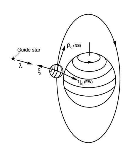
Figure 1: Basis four-vectors for Gravity Probe-B

Each gyroscope is characterized by a spin four-vector $\mathsf{S}$ that is purely spatial in the spacecraft frame ($\mbox{\boldmath$\mathsf{S}$}\cdot\mbox{\boldmath$\mathsf{u}$}=0$); this amounts to a specific choice of its center of mass. We assume that gyro torques are sufficiently small that we can treat the gyros as perfect, so that $\mathsf{S}$ is parallel transported ($\mbox{\boldmath$\mathsf{\nabla}$}_{\mbox{\boldmath$\mathsf{u}$}}{\mbox{\boldmath$\mathsf{S}$}}=0$). Then the rate of change of each component of $\mathsf{S}$ on the roll-fixed basis is given by $d(\mbox{\boldmath$\mathsf{S}$}\cdot\mbox{\boldmath$\mathsf{e}$}_{\alpha})/d\tau=\mbox{\boldmath$\mathsf{S}$}\cdot\mbox{\boldmath$\mathsf{\nabla}$}_{\mbox{\boldmath$\mathsf{u}$}}\mbox{\boldmath$\mathsf{e}$}_{\alpha}$; combining with Eqs. (4) we obtain the equation of motion for the spin components,

$$\dot{S}_{\eta_{0}} = -t_{\eta_{0}}S_{\xi}\,,$$

$$\dot{S}_{\rho_{0}} = -t_{\rho_{0}}S_{\xi}\,,$$

$$\dot{S}_{\xi} = t_{\eta_{0}}S_{\eta_{0}}+t_{\rho_{0}}S_{\rho_{0}}\,,$$ (5)

where $S_{\eta_{0}}=\mbox{\boldmath$\mathsf{S}$}\cdot\mbox{\boldmath$\mathsf{\eta}$}_{0}$ $S_{\rho_{0}}=\mbox{\boldmath$\mathsf{S}$}\cdot\mbox{\boldmath$\mathsf{\rho}$}_{0}$, and $S_{\xi}=\mbox{\boldmath$\mathsf{S}$}\cdot\mbox{\boldmath$\mathsf{\xi}$}$, with parallel definitions for $t_{\eta_{0}}$, etc., and where overdot denotes $d/d\tau$. In the absence of torques on the spacecraft ($\mbox{\boldmath$\mathsf{t}$}=0$), $\dot{S}_{\eta_{0}}=\dot{S}_{\rho_{0}}=\dot{S}_{\xi}=0$, as expected, since the gyro spins and spacecraft basis vectors will undergo identical transports through spacetime.

III Telescope pointing

The spacecraft is oriented so that the optical axis of the telescope is aligned parallel to the direction of an incoming photon from the guide star. Let $\mathsf{\lambda}$ be the null tangent vector to the incoming photon satisfying the geodesic equation $\mbox{\boldmath$\mathsf{\nabla}$}_{\mbox{\boldmath$\mathsf{\lambda}$}}\mbox{\boldmath$\mathsf{\lambda}$}=0$ with $\mbox{\boldmath$\mathsf{\lambda}$}\cdot\mbox{\boldmath$\mathsf{\lambda}$}=0$. In the spacecraft frame, the direction of the incoming photon is given by a unit normalized spatial vector which is the projection of $\mathsf{\lambda}$ onto the spacecraft basis, namely

$${\mbox{\boldmath$\mathsf{\hat{\lambda}}$}}={{\mbox{\boldmath$\mathsf{\lambda}$}}\over{(-\mbox{\boldmath$\mathsf{u}$}\cdot\mbox{\boldmath$\mathsf{\lambda}$})}}-\mbox{\boldmath$\mathsf{u}$}\,.$$ (6)

Then, using Eqs. (4) the equations of motion for the roll-fixed components of $\mathsf{\hat{\lambda}}$ are given by

$$(d/d\tau){\hat{\lambda}}_{\eta_{0}} = \epsilon^{1/2}(\mbox{\boldmath$\mathsf{\nabla}$}_{\mbox{\boldmath$\mathsf{u}$}}\mbox{\boldmath$\mathsf{\hat{\lambda}}$})\cdot\mbox{\boldmath$\mathsf{\eta}$}_{0}-t_{\eta_{0}}{\hat{\lambda}}_{\xi}\,,$$

$$(d/d\tau){\hat{\lambda}}_{\rho_{0}} = \epsilon^{1/2}(\mbox{\boldmath$\mathsf{\nabla}$}_{\mbox{\boldmath$\mathsf{u}$}}\mbox{\boldmath$\mathsf{\hat{\lambda}}$})\cdot\mbox{\boldmath$\mathsf{\rho}$}_{0}-t_{\rho_{0}}{\hat{\lambda}}_{\xi}\,,$$

$$(d/d\tau){\hat{\lambda}}_{\xi} = \epsilon^{1/2}(\mbox{\boldmath$\mathsf{\nabla}$}_{\mbox{\boldmath$\mathsf{u}$}}\mbox{\boldmath$\mathsf{\hat{\lambda}}$})\cdot\mbox{\boldmath$\mathsf{\xi}$}+t_{\eta_{0}}{\hat{\lambda}}_{\eta_{0}}+t_{\rho_{0}}{\hat{\lambda}}_{\rho_{0}}\,,$$ (7)

where we have introduced the small parameter $\epsilon^{1/2}\sim(v/c)$ to characterize the leading effects on $\mbox{\boldmath$\mathsf{\nabla}$}_{\mbox{\boldmath$\mathsf{u}$}}\mbox{\boldmath$\mathsf{\hat{\lambda}}$}$, namely aberration.

In the operation of the experiment, attitude control forces orient the spacecraft so that the telescope always points toward the apparent location of the guide star, i.e. so that $\mbox{\boldmath$\mathsf{\hat{\lambda}}$}=-\mbox{\boldmath$\mathsf{\xi}$}$, or so that ${\mbox{\boldmath$\mathsf{\hat{\lambda}}$}}\cdot\mbox{\boldmath$\mathsf{\rho}$}_{0}=\mbox{\boldmath$\mathsf{\hat{\lambda}}$}\cdot\mbox{\boldmath$\mathsf{\eta}$}_{0}=0$. This will be only approximately true because of pointing errors and occasional deliberate “dithering” of the spacecraft for operational and other reasons; these errors are expected to be on the level of a few to tens of mas. We introduce the small parameter $\delta\sim 10^{-7}$ to characterize these pointing errors. Then to drive ${\hat{\lambda}}_{\rho_{0}}$ and ${\hat{\lambda}}_{\eta_{0}}$ and their time derivatives to zero, we require attitude control torques given, from Eqs. (7), by

$$t_{\eta_{0}} = \epsilon^{1/2}{\hat{\lambda}}_{\xi}^{-1}(\mbox{\boldmath$\mathsf{\nabla}$}_{\mbox{\boldmath$\mathsf{u}$}}\mbox{\boldmath$\mathsf{\hat{\lambda}}$})\cdot{\mbox{\boldmath$\mathsf{\eta}$}}_{0}+\delta(\Delta t_{\eta_{0}})\,,$$

$$t_{\rho_{0}} = \epsilon^{1/2}{\hat{\lambda}}_{\xi}^{-1}(\mbox{\boldmath$\mathsf{\nabla}$}_{\mbox{\boldmath$\mathsf{u}$}}\mbox{\boldmath$\mathsf{\hat{\lambda}}$})\cdot{\mbox{\boldmath$\mathsf{\rho}$}}_{0}+\delta(\Delta t_{\rho_{0}})\,,$$ (8)

where $\Delta t_{\eta_{0}}$ and $\Delta t_{\rho_{0}}$ are the roll-fixed components of the order-$\delta$ residual “pointing error” and dithering torques. Substituting Eqs. (8) back into Eqs. (7), and using the fact that $\mathsf{\hat{\lambda}}$ is a normalized vector, we find that $(d/d\tau){\hat{\lambda}}_{\eta_{0}}=-\delta(\Delta t_{\eta_{0}}){\hat{\lambda}}_{\xi}$, $(d/d\tau){\hat{\lambda}}_{\rho_{0}}=-\delta(\Delta t_{\rho_{0}}){\hat{\lambda}}_{\xi}$, and $(d/d\tau){\hat{\lambda}}_{\xi}=\delta(\Delta t_{\eta_{0}}{\hat{\lambda}}_{\eta_{0}}+\Delta t_{\rho_{0}}{\hat{\lambda}}_{\rho_{0}})$. From these equations we obtain

$${\hat{\lambda}}_{\eta_{0}}(\tau)=O(\delta)\,,{\hat{\lambda}}_{\rho_{0}}(\tau)=O(\delta)\,,{\hat{\lambda}}_{\xi}(\tau)=-1+O(\delta^{2})\,.$$ (9)

Then substituting Eqs. (8) into (5), we obtain

$${\dot{S}}_{\eta_{0}} = -\epsilon^{1/2}(S_{\xi}/{\hat{\lambda}}_{\xi})(\mbox{\boldmath$\mathsf{\nabla}$}_{\mbox{\boldmath$\mathsf{u}$}}\mbox{\boldmath$\mathsf{\hat{\lambda}}$})\cdot\mbox{\boldmath$\mathsf{\eta}$}_{0}-\delta(\Delta t_{\eta_{0}})S_{\xi}\,,$$

$${\dot{S}}_{\rho_{0}} = -\epsilon^{1/2}(S_{\xi}/{\hat{\lambda}}_{\xi})(\mbox{\boldmath$\mathsf{\nabla}$}_{\mbox{\boldmath$\mathsf{u}$}}\mbox{\boldmath$\mathsf{\hat{\lambda}}$})\cdot\mbox{\boldmath$\mathsf{\rho}$}_{0}-\delta(\Delta t_{\rho_{0}})S_{\xi}\,,$$

$${\dot{S}}_{\xi} = \epsilon^{1/2}[S_{\eta_{0}}(\mbox{\boldmath$\mathsf{\nabla}$}_{\mbox{\boldmath$\mathsf{u}$}}\mbox{\boldmath$\mathsf{\hat{\lambda}}$})\cdot\mbox{\boldmath$\mathsf{\eta}$}_{0}+S_{\rho_{0}}(\mbox{\boldmath$\mathsf{\nabla}$}_{\mbox{\boldmath$\mathsf{u}$}}\mbox{\boldmath$\mathsf{\hat{\lambda}}$})\cdot\mbox{\boldmath$\mathsf{\rho}$}_{0}]{\hat{\lambda}}_{\xi}^{-1}$$ (10)

$$+\delta(\Delta t_{\eta_{0}}S_{\eta_{0}}+\Delta t_{\rho_{0}}S_{\rho_{0}})\,.$$

But since $S_{\eta_{0}}\sim S_{\rho_{0}}\sim\epsilon^{1/2}+\delta$, we have ${\dot{S}}_{\xi}\sim\epsilon+\epsilon^{1/2}\delta+\delta^{2}+\dots$, and so, choosing the vector $\mathsf{S}$ to be normalized to unity (under parallel transport it has constant norm), we can write $S_{\xi}=1+O(\epsilon,\epsilon^{1/2}\delta,\delta^{2})$. Substituting into Eq. (10), we obtain our final equation for the evolution of the gyro spin components relative to the roll-fixed spacecraft axes,

$${\dot{S}}_{\eta_{0}} = \epsilon^{1/2}(\mbox{\boldmath$\mathsf{\nabla}$}_{\mbox{\boldmath$\mathsf{u}$}}\mbox{\boldmath$\mathsf{\hat{\lambda}}$})\cdot\mbox{\boldmath$\mathsf{\eta}$}_{0}-\delta(\Delta t_{\eta_{0}})$$

$$+O(\epsilon^{3/2},\epsilon\delta,\epsilon^{1/2}\delta^{2})\,,$$

$${\dot{S}}_{\rho_{0}} = \epsilon^{1/2}(\mbox{\boldmath$\mathsf{\nabla}$}_{\mbox{\boldmath$\mathsf{u}$}}\mbox{\boldmath$\mathsf{\hat{\lambda}}$})\cdot\mbox{\boldmath$\mathsf{\rho}$}_{0}-\delta(\Delta t_{\rho_{0}})$$ (11)

$$+O(\epsilon^{3/2},\epsilon\delta,\epsilon^{1/2}\delta^{2})\,.$$

These physically measurable components $S_{\eta_{0}}$ and $S_{\rho_{0}}$ translate directly into outputs of the SQUID magnetometers. The expressions are generally covariant, and thus may be evaluated in any chosen coordinate system.

Interestingly, in this picture all the relativistic effects arise mathematically from the covariant derivative of the incoming photon world line along the spacecraft four-velocity, and not in the precessions of the gyroscope spins. This is because we have chosen the rolling spacecraft itself to define our basis; this was a natural choice because all the measuring instruments (current loops, SQUIDs) are rigidly fixed to the spacecraft. But since a rolling spacecraft is itself a gyroscope, it and the superconducting gyros precess together in the spacetime around the Earth. Hence, in this basis, the relativistic effects appear to originate elsewhere. The superconducting gyros are still crucial, of course, because, by design, they are closer to being perfect gyros, and thus are less affected by anomalous torques. Here the spacecraft plays a role similar to that of an oscillator clock that is slaved to an ultraprecise atomic standard (such as a hydrogen maser, or atom fountain clock); the oscillator may drift or be deliberately steered from time to time, but its phase can always be linked precisely back to the underlying standard. Similarly, while the spacecraft “gyro” is steered to follow the guide star as the star’s apparent location varies because of aberration and relativistic effects, the spacecraft axis direction is precisely linked to the superconducting gyros via the output of the SQUIDS.

We now turn to the relativistic and aberration effects that are being measured.

IV Post-Newtonian calculation of measurable relativistic effects

We evaluate the quantity $\mbox{\boldmath$\mathsf{\nabla}$}_{\mbox{\boldmath$\mathsf{u}$}}\mbox{\boldmath$\mathsf{\hat{\lambda}}$}$ in the post-Newtonian approximation using the parametrized post-Newtonian (PPN) framework tegp . The metric of spacetime in the solar-system rest-frame is taken to have the form

$$g_{00} = -1+2U+O(\epsilon^{2})\,,$$

$$g_{0i} = -(2+2\gamma+\frac{1}{2}\alpha_{1})V_{i}+O(\epsilon^{5/2})\,,$$

$$g_{ij} = (1+2\gamma U)\delta_{ij}+O(\epsilon^{2})\,,$$ (12)

where $\gamma$ and $\alpha_{1}$ are PPN parameters whose values depend on the theory of gravity, and where we have restricted attention to theories of gravity with suitable global conservation laws, and have ignored “preferred-frame” terms in the metric (see tegp , §9.1 for discussion of these effects). We have used a gauge analogous to harmonic gauge, instead of the conventional PPN gauge (see tegp §4.2 for discussion). For an orbiting, rotating, nearly spherical Earth, and a static, spherically symmetric Sun, the potentials $U$ and ${\bf V}$ have the form

$$U = M_{\odot}/r+M_{\oplus}/R\,,$$

$${\bf V} = M_{\oplus}{\bf v}_{\oplus}/R-\frac{1}{2}{\bf X}\times{\bf J_{\oplus}}/R^{3}\,,$$ (13)

where $M_{\odot}$ is the mass of the Sun, $M_{\oplus}$, ${\bf v}_{\oplus}$ and ${\bf J}_{\oplus}$ are the mass, velocity and angular momentum of the Earth; ${\bf X}={\bf x}-{\bf x}_{\oplus}$ and $R=|{\bf X}|$ denote the satellite-Earth vector and distance, while $\bf x$ and $r=|{\bf x}|$ denote the satellite-Sun vector and distance. In fact, the quadrupole moment of the Earth has a measurable effect on the geodetic precession and must be included; as this has been treated thoroughly elsewhere wilkins ; barker70 ; breakwell ; adler we will ignore it here.

From the geodesic equation for photons, $d\lambda^{i}/dt+(\Gamma^{i}_{\mu\nu}-\Gamma^{0}_{\mu\nu}\lambda^{i})\lambda^{\mu}\lambda^{\nu}=0$, where $\lambda^{\mu}=dx^{\mu}/dt$, we obtain the solution (see tegp §7.1 for details):

$$\lambda^{0} = 1\,,$$

$$\lambda^{i} = {n}^{i}[1-(1+\gamma)U]+{\cal D}^{i}+O(\epsilon^{3/2})\,,$$ (14)

where ${n}^{i}$ is a Cartesian unit vector describing the initial direction of the photon far from the Earth in the global PPN coordinate system, and ${\cal D}^{i}$ represents the deflection of the ray, obtained by solving the equation

$$\left({{d{\cal D}^{i}}\over dt}\right)_{{\rm along}\,n^{i}}=(1+\gamma)[\nabla^{i}U-n^{i}({\bf n}\cdot\nabla U)]\,.$$ (15)

The unit vector ${\bf n}$ points from the source toward the spacecraft, and hence may be written ${\bf n}={\bf n}_{0}+{\bf x}\cdot\nabla{\bf n}_{0}+\dots$, where ${\bf n}_{0}$ is a constant unit vector toward the solar-system barycenter and where $\nabla^{i}n_{0}^{j}=(\delta^{ij}-n_{0}^{i}n_{0}^{j})/D$, where $D$ is the distance from the solar-system barycenter to the guide star. The correction term accounts for the parallax of the guide star; for HR 8703 it amounts to about 10 mas $\sim 3\times 10^{-7}$. Because it is so small, we will treat it as effectively a pointing error term, of order $\delta$.

Letting the spacecraft have ordinary velocity $v^{i}=u^{i}/u^{0}$, where $u^{0}=1+v^{2}/2+U+O(\epsilon^{2})$, we find that the components of $\mathsf{\hat{\lambda}}$ are given by

$${\hat{\lambda}}^{0} = {\bf n}\cdot{\bf v}-[v^{2}-({\bf n}\cdot{\bf v})^{2}]+O(\epsilon^{3/2})\,,$$

$${\hat{\lambda}}^{i} = {n}^{i}-[v^{i}-n^{i}({\bf n}\cdot{\bf v})]+n^{i}[({\bf n}\cdot{\bf v})^{2}-v^{2}/2-\gamma U]$$ (16)

$$+{\cal D}^{i}+O(\epsilon^{3/2})\,.$$

To calculate the covariant quantities $(\mbox{\boldmath$\mathsf{\nabla}$}_{\mbox{\boldmath$\mathsf{u}$}}\mbox{\boldmath$\mathsf{\hat{\lambda}}$})\cdot\mbox{\boldmath$\mathsf{\eta}$}_{0}$ and $(\mbox{\boldmath$\mathsf{\nabla}$}_{\mbox{\boldmath$\mathsf{u}$}}\mbox{\boldmath$\mathsf{\hat{\lambda}}$})\cdot\mbox{\boldmath$\mathsf{\rho}$}_{0}$ in Eqs. (11), it suffices to evaluate them in the PPN coordinate system. We first evaluate $(\mbox{\boldmath$\mathsf{\nabla}$}_{\mbox{\boldmath$\mathsf{u}$}}\mbox{\boldmath$\mathsf{\hat{\lambda}}$})^{\alpha}=u^{\beta}{{\hat{\lambda}}^{\alpha}}_{;\beta}$. Calculating the Christoffel symbols from the metric (12) to the needed order, and using the fact that $dU/dt=\partial U/\partial t+{\bf v}\cdot\nabla U$, and, by virtue of the equation of motion $d{\bf v}/dt=\nabla U$, that $({\bf v}\cdot{\bf n})\nabla U=1/2\{d[{\bf v}({\bf v}\cdot{\bf n})]/dt+{\bf n}\times(\nabla U\times{\bf v})\}$, we find

$$(\mbox{\boldmath$\mathsf{\nabla}$}_{\mbox{\boldmath$\mathsf{u}$}}\mbox{\boldmath$\mathsf{\hat{\lambda}}$})^{0} = O(v\nabla U)\,,$$

$$(\mbox{\boldmath$\mathsf{\nabla}$}_{\mbox{\boldmath$\mathsf{u}$}}\mbox{\boldmath$\mathsf{\hat{\lambda}}$})^{i} = {d\over dt}\biggl{[}({\bf x}\cdot\nabla)n_{0}^{i}-v^{i}+n^{i}({\bf n}\cdot{\bf v})$$ (17)

$$+n^{i}\{({\bf n}\cdot{\bf v})^{2}-\frac{1}{2}v^{2}\}-\frac{1}{2}v^{i}({\bf n}\cdot{\bf v})+{\cal D}^{i}\biggr{]}$$

$$+\frac{1}{2}(2\gamma+1)[{\bf n}\times({\bf v}\times\nabla U)]^{i}$$

$$+(1+\gamma+\frac{1}{4}\alpha_{1})[{\bf n}\times(\nabla\times{\bf V})]^{i}$$

$$+O(U\nabla U)\,,$$

where, to the order needed, we can convert from spacecraft proper time $\tau$ to PPN coordinate time $t$.

We also need to determine the time dependence of $\mbox{\boldmath$\mathsf{\eta}$}_{0}$ and $\mbox{\boldmath$\mathsf{\rho}$}_{0}$; even though they are roll-fixed vectors, they will vary slightly because of pointing of the spacecraft to maintain alignment with the guide star. However, because $\mbox{\boldmath$\mathsf{\nabla}$}_{\mbox{\boldmath$\mathsf{u}$}}\mbox{\boldmath$\mathsf{\hat{\lambda}}$}$ is already of $O(\epsilon^{1/2})$, we only need to evaluate $\mbox{\boldmath$\mathsf{\eta}$}_{0}$ and $\mbox{\boldmath$\mathsf{\rho}$}_{0}$ to $O(\epsilon^{1/2})$, which means accounting only for the effects of aberration-induced torques. Substituting Eqs. (8) into (4), and using the fact that $\mathsf{\xi}$, $\mbox{\boldmath$\mathsf{\rho}$}_{0}$, $\mbox{\boldmath$\mathsf{\eta}$}_{0}$, and $\mathsf{u}$ form an orthonormal tetrad, we obtain

$$\mbox{\boldmath$\mathsf{\nabla}$}_{\mbox{\boldmath$\mathsf{u}$}}\mbox{\boldmath$\mathsf{\eta}$}_{0} = \epsilon^{1/2}\mbox{\boldmath$\mathsf{\nabla}$}_{\mbox{\boldmath$\mathsf{u}$}}\mbox{\boldmath$\mathsf{\hat{\lambda}}$}\cdot\mbox{\boldmath$\mathsf{\eta}$}_{0}\mbox{\boldmath$\mathsf{\xi}$}+O(\delta)\,,$$

$$\mbox{\boldmath$\mathsf{\nabla}$}_{\mbox{\boldmath$\mathsf{u}$}}\mbox{\boldmath$\mathsf{\rho}$}_{0} = \epsilon^{1/2}\mbox{\boldmath$\mathsf{\nabla}$}_{\mbox{\boldmath$\mathsf{u}$}}\mbox{\boldmath$\mathsf{\hat{\lambda}}$}\cdot\mbox{\boldmath$\mathsf{\rho}$}_{0}\mbox{\boldmath$\mathsf{\xi}$}+O(\delta)\,,$$

$$\mbox{\boldmath$\mathsf{\nabla}$}_{\mbox{\boldmath$\mathsf{u}$}}\mbox{\boldmath$\mathsf{\xi}$} = \epsilon^{1/2}(-\mbox{\boldmath$\mathsf{\nabla}$}_{\mbox{\boldmath$\mathsf{u}$}}\mbox{\boldmath$\mathsf{\hat{\lambda}}$}+\mbox{\boldmath$\mathsf{\nabla}$}_{\mbox{\boldmath$\mathsf{u}$}}\mbox{\boldmath$\mathsf{\hat{\lambda}}$}\cdot\mbox{\boldmath$\mathsf{u}$}\mbox{\boldmath$\mathsf{u}$}+\mbox{\boldmath$\mathsf{\nabla}$}_{\mbox{\boldmath$\mathsf{u}$}}\mbox{\boldmath$\mathsf{\hat{\lambda}}$}\cdot\mbox{\boldmath$\mathsf{\xi}$}\mbox{\boldmath$\mathsf{\xi}$})$$ (18)

$$+O(\delta)\,.$$

We use the fact that, for each of these three vectors, $(\mbox{\boldmath$\mathsf{\nabla}$}_{\mbox{\boldmath$\mathsf{u}$}}\mbox{\boldmath$\mathsf{e}$}_{(\alpha)})^{\beta}=d{e}_{(\alpha)}^{\beta}/d\tau+\Gamma^{\beta}_{\gamma\delta}e_{(\alpha)}^{\gamma}u^{\delta}$, substitute the Christoffel symbols and Eqs. (17), and integrate, to obtain

$$(\eta_{0})^{0}(t) = {\bf v}\cdot{\bf{\bar{\eta}}}_{0}+O(\epsilon,\delta)\,,$$

$$(\eta_{0})^{i}(t) = ({\bar{\eta}}_{0})^{i}-{\bf v}\cdot{\bf{\bar{\eta}}}_{0}{\bar{\xi}}^{i}+O(\epsilon,\delta)\,,$$

$$(\rho_{0})^{0}(t) = {\bf v}\cdot{\bf{\bar{\rho}}}_{0}+O(\epsilon,\delta)\,,$$

$$(\rho_{0})^{i}(t) = ({\bar{\rho}}_{0})^{i}-{\bf v}\cdot{\bf{\bar{\rho}}}_{0}{\bar{\xi}}^{i}+O(\epsilon,\delta)\,,$$

$$\xi^{0}(t) = {\bf v}\cdot{\bf{\bar{\xi}}}+O(\epsilon,\delta)\,,$$

$$\xi^{i}(t) = {\bar{\xi}}^{i}+v^{i}-{\bar{\xi}}^{i}{\bf v}\cdot{\bf\bar{\xi}}+O(\epsilon,\delta)\,,$$ (19)

where ${\bf{\bar{\eta}}}_{0}$, ${\bf{\bar{\rho}}}_{0}$ and ${\bf{\bar{\xi}}}$ are spatial 3-vectors in the PPN frame that describe the orientation of the spacecraft at a chosen initial moment of time. They are orthonormal in the Cartesian sense to $O(\epsilon)$. We have used the fact, obtainable from Eq. (9), that ${\bf n}=-{\bf{\bar{\xi}}}+O(\epsilon,\delta)$, ${\bf n}\cdot{\bf{\bar{\eta}}}_{0}=O(\epsilon,\delta)$ and ${\bf n}\cdot{\bf{\bar{\rho}}}_{0}=O(\epsilon,\delta)$.

Substituting Eqs. (17) and (19) into (11), converting from $d/d\tau$ to $d/dt$ using the property that $\tau=t[1+O(\epsilon)]$, and integrating with respect to $t$, we obtain, finally

$$S_{\eta_{0}} = S_{\eta_{0}}(0)-\epsilon^{1/2}{\bf v}\cdot{\bf{\bar{\eta}}}_{0}$$

$$+\epsilon\left(\frac{1}{2}{\bf v}\cdot{\bf{\bar{\eta}}}_{0}{\bf v}\cdot{\bf{\bar{\xi}}}+{\bf{\cal H}}\cdot{\bf{\bar{\eta}}}_{0}+{\bf{\cal D}}\cdot{\bf{\bar{\eta}}}_{0}\right)$$

$$+\delta(D^{-1}{\bf x}\cdot{\bf{\bar{\eta}}}_{0}-{\cal T}_{\eta_{0}})$$

$$+O(\epsilon^{3/2},\epsilon\delta,\epsilon^{1/2}\delta^{2})\,,$$

$$S_{\rho_{0}} = S_{\rho_{0}}(0)-\epsilon^{1/2}{\bf v}\cdot{\bf\bar{\rho}}_{0}$$ (20)

$$+\epsilon\left(\frac{1}{2}{\bf v}\cdot{\bf{\bar{\rho}}}_{0}{\bf v}\cdot{\bf{\bar{\xi}}}+{\bf{\cal H}}\cdot{\bf{\bar{\rho}}}_{0}+{\bf{\cal D}}\cdot{\bf{\bar{\rho}}}_{0}\right)$$

$$+\delta(D^{-1}{\bf x}\cdot{\bf{\bar{\rho}}}_{0}-{\cal T}_{\rho_{0}})$$

$$+O(\epsilon^{3/2},\epsilon\delta,\epsilon^{1/2}\delta^{2})\,.$$

The first term in Eqs. (20) is the initial misalignment of the spin with the spacecraft axis, which is expected to be smaller than one arcsecond. The next term, of order $\epsilon^{1/2}$, and the first of the $O(\epsilon)$ terms, are the aberration term and its relativistic correction. The term involving ${\bf{\cal H}}$ is the integrated relativistic precession projected onto ${\bf{\bar{\eta}}}_{0}$ and ${\bf{\bar{\rho}}}_{0}$, given by ${\bf{\cal H}}=\int^{t}(d{\bf{\cal H}}/dt)dt$, where $d{\bf{\cal H}}/dt$ is the precession rate given by

$${d{\bf{\cal H}}\over dt}=-\frac{1}{2}(2\gamma+1){\bf{\bar{\xi}}}\times({\bf v}\times\nabla U)-(1+\gamma+\frac{1}{4}\alpha_{1}){\bf{\bar{\xi}}}\times(\nabla\times{\bf V})\,.$$ (21)

The terms ${\bf{\cal D}}\cdot{\bf{\bar{\eta}}}_{0}$ and ${\bf{\cal D}}\cdot{\bf{\bar{\rho}}}_{0}$ in Eqs. (20) denote the contribution of the deflection of light. The $O(\delta)$ terms ${\cal T}_{\eta_{0}}$ and ${\cal T}_{\rho_{0}}$ denote the integrated angular offset caused by pointing errors, while the terms $D^{-1}{\bf x}\cdot{\bf{\bar{\eta}}}_{0}$ and $D^{-1}{\bf x}\cdot{\bf{\bar{\rho}}}_{0}$ denote the effects of parallax. The spatial vectors defined in Eqs. (20) are referred to the solar-system-fixed PPN coordinate system. However, to the order needed, we can write ${\bf v}={\bf v}_{\oplus}+{\bf v}_{s}+O(\epsilon^{3/2})$, where ${\bf v}_{\oplus}$ is the Earth’s orbital velocity relative to the Sun, and ${\bf v}_{s}$ is the spacecraft’s velocity relative to the Earth. Furthermore, the components of the various 3-vectors in the solar-system basis are equal to the respective components in a non-rotating Earth-comoving basis, apart from corrections of order $\epsilon$; hence to the order needed in Eqs. (20) we can treat all spatial vectors as defined in the geocentric basis.

V Discussion of Relativistic Effects

The first non-constant term in Eqs. (20) is the aberration of starlight, consisting of both an annual aberration with amplitude of ${\bf v}_{\oplus}\sim 20$ arcseconds, and an orbital aberration with amplitude ${\bf v}_{s}\sim 5$ arcseconds. But because the position of the guide star can be determined from VLBI and the orbit of the earth and spacecraft can be determined from the ephemeris and GPS to high accuracy, these terms may be predicted to an accuracy better than that needed to measure the relativistic effects. Furthermore, their variation with time over a year can be separated from the variation of the relativistic terms, hence the aberration can be used to determine the “scale factor” that relates the output of the SQUIDs (the actual data) to the desired angles $S_{\eta_{0}}$ and $S_{\rho_{0}}$. The second term in Eqs. (20) is the relativistic correction to aberration, whose orbital part dominates, with amplitude $\frac{1}{2}v_{\oplus}^{2}\sin\beta\sim 0.4$ mas ($\beta$ is the ecliptic latitude of the guide star), which is comparable to the accuracy goal of the experiment; this term must be included in the data analysis stumpff . Terms of order $v_{\oplus}v_{s}$ and $v_{s}^{2}$ and terms cubic in $v$ can be ignored.

For the relativistic precession terms, $d{\bf{\cal H}}/dt$ can be separated into various contributions using Eqs. (13):

$${{d{{\bf\cal H}}}\over dt} = \left\{\frac{1}{4}(2+\alpha_{1}){M_{\oplus}\over R^{3}}{\bf v}_{\oplus}\times{\bf X}-\frac{1}{2}(2\gamma+1){M_{\odot}\over r^{3}}{\bf v}_{s}\times{\bf x}\right.$$ (22)

$$\left.-\frac{1}{2}(2\gamma+1){M_{\odot}\over r^{3}}{\bf v}_{\oplus}\times{\bf x}-\frac{1}{2}(2\gamma+1){M_{\oplus}\over R^{3}}{\bf v}_{s}\times{\bf X}\right.$$

$$\left.-\frac{1}{2}(\gamma+1+\frac{1}{4}\alpha_{1})\left[{{{\bf J}_{\oplus}-3{\bf N}{\bf J}_{\oplus}\cdot{\bf N}}\over R^{3}}\right]\right\}\times{\bf{\bar{\xi}}}\,,$$

where ${\bf N}={\bf X}/R$. Since $\cal H$ and ${\bf\bar{\xi}}$ both refer to the direction of the spins, this equation has the general form $d{\bf S}/dt={\bf\Omega}\times{\bf S}$, so that the quantity in braces in Eq. (22) can be regarded as the precession rate vector.

The first two terms produce periodic contributions to the signal at the frequencies $\omega_{s}\pm\omega_{\oplus}$, where $\omega_{s}$ and $\omega_{\oplus}\ll\omega_{s}$ are the orbital angular frequencies of the spacecraft and Earth, respectively. Integrated over time, these contribute periodic terms at approximately the orbital frequency with amplitudes of $v_{\oplus}M_{\oplus}/2R^{2}\omega_{s}\sim v_{\oplus}v_{s}/2\sim 0.3$ mas and $v_{s}M_{\odot}/r^{2}\omega_{s}\sim v_{\oplus}^{2}(R/r)\sim 10^{-4}$ mas, respectively. Averaged over time, these are negligible.

The third term may be evaluated to sufficient accuracy at the center of the Earth rather than at the satellite; treating the Earth’s orbit as circular yields a signal that grows at the constant rate of $(3/2)v_{\oplus}^{2}\omega_{\oplus}({\bf h}\times{\bf{\bar{\xi}}})\sim 19$ mas/yr in a direction perpendicular to ${\bf h}$, the normal to the ecliptic plane wilkins ; barkeroconnell2 . This term is the solar geodetic effect (sometimes called the de Sitter precession); it is responsible for an analogous precession in the lunar orbit that has been measured to around 0.7 % using Lunar laser ranging williams .

The fourth term is the main geodetic effect, at the constant rate of $(3/2)v_{s}^{2}\omega_{s}({\bf h}^{\prime}\times{\bf{\bar{\xi}}})\sim 6600$ mas/yr, in a direction perpendicular to ${\bf h}^{\prime}$, the normal to the orbital plane. Note that if ${\bf{\bar{\eta}}}_{0}$ is chosen to be the EW basis vector, which is perpendicular to the polar orbit, then the main geodetic effect does not appear in the output $S_{\eta_{0}}$, in other words it produces a purely $S_{\rho_{0}}$, or NS signal. There is an additional contribution to this precession arising from the Earth’s oblateness at about 7 mas/yr, which must be taken into account wilkins ; barker70 ; oconnell ; barkeroconnell3 ; breakwell ; adler

The final term in Eq. (22) is the Lense-Thirring or frame-dragging effect. It has both a constant term and a periodic term at twice the orbital frequency, but for a circular polar orbit, it produces an orbit-averaged constant rate of ${\bf J}_{\oplus}\times{\bf{\bar{\xi}}}/2R^{3}=J_{\oplus}\cos\delta/2R^{3}\sim 41\cos\delta$ mas/yr, where $\delta$ is the declination of the guide star. If the plane of the polar orbit is oriented so that the guide star location is in the orbital plane, then the signal is purely $S_{\eta_{0}}$, or EW.

The next term in Eqs. (20) is the deflection of light. For the ecliptic latitude of the guide star, this gives a maximum deflection caused by the Sun of around 20 mas, once in the one-year mission. This effect can be included as a term to be estimated in the data analysis – studies by the GP-B team indicate that it could be measured to about one percent – or it can calculated a priori using general relativity and the known parameters of the Earth’s orbit and the guide star location. Because the guide star will be occulted by the Earth, the Earth will also contribute a once-per-orbit deflection of around 0.5 mas (which will compete with deflection caused by propagation of the signal through the Earth’s atmosphere). Because it averages to zero, this effect can be ignored.

These relativistic terms, geodetic precession, frame dragging and deflection of light, have been calculated using the specific assumptions and constraints inherent in the PPN framework. An alternative, more phenomenological viewpoint, would be to regard each as an independent effect with a separate phenomenological parameter to be measured in the data analysis.

The remaining terms in Eqs. (20) are of order $\delta$. The parallax term caused by the Earth’s motion (around 10 mas) must be taken into account, while that due to the satellite’s orbit is negligible. Finally the pointing error terms will be controlled to better than 20 mas (rms), and in any event will be measured directly by the telescope; all that is needed then is a sufficiently accurate calibration (via deliberate dithering of the spacecraft axis by known amounts) to convert telescope readout signals to the appropriate contributions ${\cal T}_{\eta_{0}}$ and ${\cal T}_{\rho_{0}}$ to $S_{\eta_{0}}$ and $S_{\rho_{0}}$.

VI Conclusions

We have carried out a covariant calculation of the measurable output of an orbiting gyroscope experiment, and shown that the result may be expressed in terms of contributions that can be calculated consistently using an Earth-based coordinate frame. The dominant contributions that are detectable within the stated 0.4 mas/yr accuracy of the GB-P mission are: the aberration of starlight and its special relativistic correction, the general relativistic geodetic precession (due both to the Earth and to the Sun) and the general relativistic frame-dragging. The results are in agreement with other, non-covariant calculations, including numerous unpublished calculations and simulations carried out by the GP-B team in the course of developing the data analysis sytem for the mission. Because all measurements are referred to instruments fixed on a rolling spacecraft, the measurable relativistic effects enter mathematically via their effect on the apparent direction of the light from the guide star.

*

Appendix A Effect of aberration on measurement of roll phase

The actual signals measured on the GP-B spacecraft are $S_{\eta}$ and $S_{\rho}$; these are then converted to roll-fixed signals in the data analysis by forming the combination

$$S_{\eta_{0}} = S_{\eta}\cos\theta-S_{\rho}\sin\theta\,,$$

$$S_{\rho_{0}} = S_{\eta}\sin\theta+S_{\rho}\cos\theta\,,$$ (23)

where $\theta$ is the spacecraft roll phase. In practice this is determined using a pair of star-trackers fixed to the spacecraft platform directed roughly perpendicular to the roll axis, that continually compare the spacecraft orientation to a library of known stellar positions, and provide a phase accurate to a few arcseconds. The angle $\theta$ is the accumulated phase in the onboard rotating frame since the initial state, so that any error in measuring $\theta$ relative to its “true” value will generate corrections to the roll-fixed outputs given by $\Delta S_{\eta_{0}}\approx-S_{\rho_{0}}\Delta\theta$, and $\Delta S_{\rho_{0}}\approx S_{\eta_{0}}\Delta\theta$.

Consider a star-tracker whose optical axis is parallel to the $\mathsf{\eta}$ vector. It will record a star when the incoming projected world line of the photon is anti-parallel to $\mathsf{\eta}$. i.e. when $\mbox{\boldmath$\mathsf{\eta}$}^{\prime}=-\mbox{\boldmath$\mathsf{\hat{\lambda}}$}=-{\bf n}+{\bf v}-{\bf n}{\bf n}\cdot{\bf v}$. In the absence of spacecraft motion, we would have $\mbox{\boldmath$\mathsf{\eta}$}=-{\bf n}$. If $\theta^{\prime}$ is the measured roll phase and $\theta$ is the “true” roll-phase (without aberration), then

$$\cos\theta^{\prime} = \mbox{\boldmath$\mathsf{\eta}$}^{\prime}\cdot\mbox{\boldmath$\mathsf{\eta}$}_{0}$$ (24)

$$= \cos\theta+{\bf v}\cdot{\bf\rho}\sin\theta\,,$$

hence $\Delta\theta={\bf v}\cdot{\bf\rho}={\bf v}\cdot{\bf\rho}_{0}\cos\theta-{\bf v}\cdot{\bf\eta}_{0}\sin\theta$. But since $S_{\eta_{0}}=S_{\eta_{0}}(0)-\epsilon^{1/2}{\bf v}\cdot{\bf{\bar{\eta}}}_{0}+O(\epsilon,\delta)$, with a parallel expression for $S_{\rho_{0}}$, the product $S_{\eta_{0}}\Delta\theta$ is of magnitude at most $10^{-8}\sim 2$ mas, but most importantly is periodic at the roll frequency, and averages to zero. Aberration will be taken into account in determination of roll phase from the star trackers.

References

- (1) C. W. F. Everitt, in Near Zero: New Frontiers of Physics, edited by J. D. Fairbank, B. S. Deaver, Jr., C. W. F. Everitt and P. F. Michelson (Freeman, San Francisco, 1988), pp. 587 - 639.
- (2) See the project website at http://einstein.stanford.edu.
- (3) C. W. F. Everitt, W. M. Fairbank and L. I. Schiff, in The Significance of Space Research for Fundamental Physics, ESRO SP-52, edited by A. F. Moore and V. Hardy (European Space Research Organization, Paris, 1971), p. 33.
- (4) G. E. Pugh, Weapons System Evaluation Group, Research Memorandum No. 111, Department of Defense, 1959 (unpublished)
- (5) L. I. Schiff, Phys. Rev. Lett. 4, 215 (1960).
- (6) L. I. Schiff, Proc. Nat. Acad. Sci. (U.S.A.) 46, 871 (1960).
- (7) D. C. Wilkins, Ann. Phys. (N.Y.) 61, 277 (1970).
- (8) W. Rindler and V. Perlick, Gen. Relativ. Gravit. 22, 1067 (1990).
- (9) D. Tsoubelis, A. Economou and E. Stoghianidis, Phys. Rev. D 36, 1045 (1987).
- (10) B. R. Iyer and C. V. Vishveshwara, Phys. Rev. D 48, 5706 (1993).
- (11) R. T. Jantzen, P. Carini and D. Bini, Ann. Phys. (N.Y) 215, 1 (1992).
- (12) J. L. Hernández-Pastora, J. Martín and E. Ruiz, preprint (gr-qc/0009062).
- (13) P. Teyssandier, Phys. Rev. D 16, 946 (1977); ibid. 18, 1037 (1978).
- (14) B. M. Barker and R. F. O’Connell, Gen. Relativ. Gravit. 11, 149 (1979).
- (15) J. V. Breakwell, in Near Zero: New Frontiers of Physics, edited by J. D. Fairbank, B. S. Deaver, Jr., C. W. F. Everitt and P. F. Michelson (Freeman, San Francisco, 1988), pp. 685-690.
- (16) R. J. Adler and A. S. Silbergleit, Int. J. Theor. Phys. 39, 1291 (2000).
- (17) S. Weinberg, Gravitation and Cosmology (Wiley, New York, 1971).
- (18) C. W. Misner, K. S. Thorne and J. A. Wheeler, Gravitation (Freeman, San Francisco, 1972).
- (19) C. M. Will, Theory and Experiment in Gravitational Physics (Cambridge University Press, Cambridge, 1993).
- (20) M. H. Soffel, Relativity in Celestial Mechanics and Geodesy (Springer-Verlag, Berlin, 1989).
- (21) V. A. Brumberg, Essential Relativistic Celestial Mechanics (Adam Hilger, Bristol, 1991).
- (22) N. Ashby and B. Shahid-Saless, Phys. Rev. D 42, 1118 (1990).
- (23) Sans serif bold symbols here denote four-vectors.
- (24) Since is not strictly an angular momentum vector, is not strictly a torque; in any event, its precise form will not be needed.
- (25) B. M. Barker and R. F. O’Connell, Phys. Rev. D 2, 1428 (1970).
- (26) P. Stumpff, Astron. Astrophys. 84, 257 (1980).
- (27) B. M. Barker and R. F. O’Connell, Phys. Rev. Lett. 25, 1511 (1970).
- (28) J. G. Williams, X X Newhall, and J. O. Dickey, Phys. Rev. D 53, 6730 (1996).
- (29) R. F. O’Connell, Astrophys. Sp. Sci. 4, 199 (1969).
- (30) B. M. Barker and R. F. O’Connell, Phys. Rev. D 6, 956 (1972).