Dynamical system approach to cosmological models with a varying speed of light

Abstract

Methods of dynamical systems have been used to study homogeneous and isotropic cosmological models with a varying speed of light (VSL). We propose two methods of reduction of dynamics to the form of planar Hamiltonian dynamical systems for models with a time dependent equation of state. The solutions are analyzed on two-dimensional phase space in the variables $(x,\dot{x})$ where $x$ is a function of a scale factor $a$. Then we show how the horizon problem may be solved on some evolutional paths. It is shown that the models with negative curvature overcome the horizon and flatness problems. The presented method of reduction can be adopted to the analysis of dynamics of the universe with the general form of the equation of state $p=\gamma(a)\epsilon$. This is demonstrated using as an example the dynamics of VSL models filled with a non-interacting fluid. We demonstrate a new type of evolution near the initial singularity caused by a varying speed of light. The singularity-free oscillating universes are also admitted for positive cosmological constant. We consider a quantum VSL FRW closed model with radiation and show that the highest tunnelling rate occurs for a constant velocity of light if $c(a)\propto a^{n}$ and $-1<n\leq 0$. It is also proved that the considered class of models is structurally unstable for the case of $n<0$.

I Introduction

Although the standard cosmological model is usually believed to be a correct picture of our universe Kolb and Turner (1990) it has still some difficulties among which the flatness and horizon problems are most widely known. The existence of the large-scale structure in the universe extending to the limit of the deepest surveys is another mystery. Its very presence implies the appearance of some seeds for this structure in the early universe. In the standard big-bang scenario they should be built in, which is rather an undesired feature of the theory. Therefore, so great attention has been paid to inflationary universe models which, albeit invoking an exotic (if not hypothetical) physics, were able to provide at least some hope for a consistent explanation of both flatness and horizon problems as well as the origin of seeds for the large-scale structure. The results of the early universe physics lead us to expect the occurrence of phase transitions when the universe was young, hot, and dense.

The varying speed of light (VSL) cosmology, seen as an alternative to the inflation theory, was proposed by Moffat Moffat (1993a, b) who conjectured that a spontaneous breaking of the local Lorentz invariance and diffeomorphism invariance associated with a first order phase-transition can lead to the variation of the speed of light in the early universe. This idea was revived by Albrecht and Magueijo Albrecht and Magueijo (1999) and was given further consideration by Barrow Barrow (1999, 2000). Barrow showed that the conception of VSL can lead to the solution of flatness, horizon, and monopole problems if the speed of light falls at an appropriate rate. The dynamics of VSL was widely studied in theoretical as well as empirical contexts Albrecht (1999); Alexander (2000); Avelino and Martins (1999); Avelino et al. (2000); Barrow and Magueijo (1998, 1999); Bassett et al. (2000); Clayton and Moffat (1999); Drummond (1999); Moffat (1998).

The main motivation for the study of VSL models is to seek explanations for some unusual properties of the universe and to overcome some of the shortcomings of inflation scenario Barrow (2002). In particular, there is an empirical evidence of varying with time the fine structure constant in the context of the consistency of quasar absorption spectra Webb et al. (1999). Moreover, unlike the inflation the VSL theory provides a solution of the cosmological constant problem. However, it cannot solve the isotropy problem. It is also interesting to evaluate the power of this model to explain the acceleration problem Perlmutter et al. (1998); Schmidt et al. (1998).

Of course, the VSL model as well as other models discussed in the literature have an ad hoc element (variable $c$) not yet firmly founded within any existing physical theories. This feature does not seems to be so exotic to discard these models from discussion in the scientific community. Some brilliant arguments justifying this approach are given by Albrecht and Magueijo Albrecht and Magueijo (1999).

The varying speed of light models which provide decent fits to the real universe are characterized by the speed of light or gravitational coupling which varies with time in the very early universe but is nearly constant today. Because there are stringent bounds on how fast these constants can vary with time after the first few seconds, the models which dynamics we study in the paper are only relevant in the very early universe. This should be made very clear by using the phase space approach and its tools for classifying the qualitative types of solutions Bogoyavlensky (1985); Szydłowski and Biesiada (1990).

The present paper is a continuation of previous papers Biesiada and Szydłowski (2000); Biesiada (2003) on the dynamics of VSL cosmology. We introduce a simple framework which allows to study the dynamics of VSL models in a general way, independent of any specific assumption about the equation of state, or the behaviour of the scale factor $a(t)$ near the spatial singularity. We formulate a VSL Friedmann-Robertson-Walker cosmology as a two-dimensional dynamical system and we discuss its properties on phase portraits where trajectories represent all solutions for all physically admissible initial conditions. The methods of dynamical systems allow to indicate how the existence of certain desired physical effects depends on the choice of initial conditions and to analyse how these initial conditions determining the corresponding solutions are distributed in the phase space.

Our main goal was to perform a global analysis of the dynamics of VSL cosmological models. We avoid the assumption of power type evolution in the VSL models, which are represented by critical points (singular solutions) in the phase space. We analyse the dynamics of the models on the phase plane and discuss how different trajectories representing non-singular solutions can solve cosmological puzzles. We conclude that models with the negative curvature and positive cosmological constant are preferred (in the sense that they have the largest set of initial conditions leading to the solution of flatness and horizon problems).

On the other hand we present two arguments which distinguish the FRW models with constant velocity of light. The theoretical one is that the VSL FRW models are structurally unstable if $c(a)\propto a^{n}$ and $n<0$ contrary to classical FRW models. The quantum mechanical one is that if a closed universe was born from a quantum fluctuation via the quantum tunnelling process then the most probable universe is that with $c=\text{const}$. In this interval the potential function preserves its classical character and the universe tunnels from a zero size.

The dynamics of considered cosmological models is reduced to the dynamics of a unit mass particle in one-dimensional potential. Then different physical properties like flatness, horizon and cosmological contant problems can be formulated in terms of the diagram of potential function of the system.

II The method of the dynamical system stability

First of all, equations describing a cosmological model should be reduced to the form of a dynamical system

$$\dot{x}_{i}=\frac{dx_{i}}{dt}=f_{i}(x_{1},\ldots,x_{n}),\quad i=1,\ldots,n$$

in such a way that the solution with a static microspace (or other solutions of interest) is a critical point of the system $(x_{1}^{*},\ldots,x_{n}^{*})$, i.e. for every $i$, $f_{i}(x_{1}^{*},\ldots,x_{n}^{*})=0$ $(i=1,\ldots,n)$.

If a critical point is non-degenerate, i.e., at this point all real parts of the eigenvalues $\mathop{\mathrm{Re}}\lambda_{i}$ of the linearization matrix

$$A_{j}^{i}=\left.\frac{\partial f_{i}}{\partial x_{j}}\right|_{x=x^{*}}$$

do not vanish, then there is a one-to-one continuous mapping of a neighbourhood of this point which transforms trajectories of the original system into trajectories of the linearized system

$$\frac{dx_{i}}{dt}=\sum\frac{\partial f_{i}}{\partial x_{j}}(x^{*})(x_{j}-x_{j}^{*}).$$

In this sense, the qualitative behaviour of the original system is equivalent to the behaviour of its linearized part. If $(\xi_{i}^{1},\ldots,\xi_{i}^{n})$ are eigenvectors of the linearization matrix $A_{j}^{i}$, the solution of the linearized system has, in general, the following form

$$x_{i}(t)-x_{i}^{*}=\mathop{\mathrm{Re}}\sum_{k=1}^{n}C_{k}\xi_{i}^{k}e^{\lambda_{k}t}$$

where $C_{k}$ are constants. A non-degenerate critical point is called an attracting point if, for all eigenvalues, $\mathop{\mathrm{Re}}\lambda_{i}<0$. In this case, all trajectories from a neighbourhood of this point go to it when $t\to\infty$. A non-degenerate critical point is called an repulsing point if, for all eigenvalues, $\mathop{\mathrm{Re}}\lambda_{i}>0$. In this case, all trajectories from a neighbourhood of this point go to it when $t\to-\infty$. A non-degenerate critical point is said to be an unstable saddle point and if a dynamical system has, at $(x_{1}^{*},\ldots,x_{n}^{*})$, $d$ eigenvalues with positive real parts and $n-d$ eigenvalues with negative real parts $(d=1,\ldots,n-1)$.

When investigating the stability of solutions with a static microspace the following theorem proves to be of special interest. If $x^{*}$ is a non-degenerate critical point and if the dynamical system has, at $x^{*}$, $d$ eigenvalues $\lambda_{1},\dots,\lambda_{d}$ with negative real parts, then there exists (locally) an invariant $d$-dimensional stable manifold $W^{d}_{\text{st}}$, on which all trajectories of the system go to $x^{*}$ as $t\to\infty$. (A manifold $M$ is said to be an invariant manifold of a system if every trajectory passing through a non-degenerate point of $M$ lies entirely in $M$ (for $-\infty<t<+\infty$). For every such solution, there exists the asymptotic

$$\lim_{t\to\infty}t^{-1}\ln\left\{\sum_{j=1}^{n}[x_{j}(t)-x_{j}^{*}]^{2}\right\}^{1/2}=\alpha_{i}$$ (1)

for a certain $i$. Similarly, if at the critical point $x^{*}$ the system has $k$ eigenvalues with positive real parts then there exists an invariant $k$-dimensional unstable manifold $W^{k}_{\text{unst}}$ on which all trajectories go away from the critical point Bogoyavlensky (1985).

From the above theorem follows that, for a saddle point, there are two invariant manifolds $W^{d}_{\text{st}}$ and $W^{n-d}_{\text{unst}}$ containing this point and filled with trajectories (separatrices) going to and going away from the critical point. All other trajectories (not contained in $W^{d}_{\text{st}}$ or in $W^{n-d}_{\text{unst}}$) do not meet the critical point in question.

For the complete construction of phase portraits in a plane it is necessary to know how trajectories of dynamical system behave at infinity. Let us take as an example the two-dimensional system

$$\dot{x} =P(x,y)$$ (2)

$$\dot{y} =Q(x,y).$$ (3)

In the case of polynomial right-hand sides one usually introduces projective coordinates, eg. $z=1/x$, $u=y/x$ or $v=1/y$, $w=x/y$. Two maps $(z,u)$ and $(v,w)$ are equivalent if and only if $u\neq 0$ and $v\neq 0$. Infinitely distant points of $(x,y)$-plane correspond to a circle $S^{1}$ which can be covered by two lines $z=0$, $-\infty<u<\infty$ and $w=0$, $-\infty<v<\infty$. The original system in the projective coordinates $(z,u)$ and after the time reparametrization $\tau\to\tau_{1}\colon d\tau_{1}=xd\tau$ assumes the form

$$\dot{z} =zP^{*}(z,u)$$ (4)

$$\dot{u} =Q^{*}(z,u)-uP^{*}(z,u)$$ (5)

where

$$P^{*}(z,u) =z^{2}P(1/z,u/z)$$

$$Q^{*}(z,u) =z^{2}Q(1/z,u/z)$$

and dot denotes differentiation with respect to new time $\tau_{1}$.

On a similar way, in the projective coordinates $(v,w)$ and in the new time $\tau_{2}\colon d\tau_{2}=yd\tau$ we obtain

$$\dot{v} =-vQ^{*}(v,w)$$ (6)

$$\dot{w} =P^{*}(v,w)-wQ^{*}(v,w)$$ (7)

where

$$P^{*}(v,w) =v^{2}P(1/v,w/v)$$

$$Q^{*}(v,w) =v^{2}Q(1/v,w/v)$$

and dot denotes differentiation with respect to time $\tau_{2}$.

The idea of structural stability was introduced by Andronov and Pontryagin Andronov and Pontryagin (1937). A dynamical system $S$ is said to be structurally stable if there exist dynamical systems in the space of all dynamical systems which are close, in the metric sense, to $S$ or are topologically equivalent to $S$. Instead of finding and analyzing an individual solution of a model, a space of all possible solutions is investigated. A given physical property is believed to be ‘realistic’ if it can be attributed to large subsets of models within a space of all possible solutions or if it possesses a certain stability, i.e., if it is also shared by a slightly perturbed model. There is a well established opinion among specialists that realistic models should be structurally stable. What does the structural stability mean in physics? The problem is in principle open in higher than 2-dimensional case where according to Smale there are large subsets of structurally unstable systems in the space of all dynamical systems Smale (1980). For 2-dimensional dynamical systems, as in the considered case, the Peixoto’s theorem says that structurally stable dynamical systems on compact manifolds form open and dense subsets in the space of all dynamical systems on the plane. Therefore, it is reasonable to require the model of a real 2-dimensional problem to be structurally stable.

In our further considerations we will investigate the dynamics of dynamical systems in a finite domain of phase space as well as at infinity. At this point we would like to recommend the presentation of the actual state of the art in the field of application of the dynamical systems to general relativity Wainwright and Ellis (1997).

III Basic equations of the theory

Albrecht and Magueijo Albrecht and Magueijo (1999) and Barrow Barrow (1999) set up a useful framework to discuss the VSL models assuming that the time variable $c$ should not introduce changes in the curvature terms of the gravitational field equations and that the Einstein equations must hold. Because varying $c$ breaks the Lorentz invariance the VSL cosmology requires a specific reference frame (including a specific choice of a time coordinate) in which changes in the field equations are minimal and one postulates it to coincide with the cosmological comoving frame.

In the case of the VSL version of the FRW models (with $\Lambda=0$) the scale factor obeys the following dynamical equations

$$\left(\frac{\dot{a}}{a}\right)^{2}=\frac{8\pi G(t)\rho}{3}-\frac{Kc^{2}(t)}{a^{2}(t)}$$ (8)

$$\frac{\ddot{a}(t)}{a}=-\frac{4\pi G(t)}{3}\left(\rho+\frac{3p}{c^{2}(t)}\right).$$ (9)

Equation (9) is called the Raychaudhuri equation and from the above system one can build a generalized conservation equation

$$\dot{\rho}+3\frac{\dot{a}}{a}\left(\rho+\frac{p}{c^{2}(t)}\right)=-\rho\frac{\dot{G}}{G}+\frac{3Kc^{2}}{8\pi Ga^{2}}\frac{\dot{c}}{c}$$ (10)

in which time dependence of fundamental constants was taken into account explicitly. Alternatively one can think of the Raychaudhuri equation together with the generalized conservation equation as of a fundamental system to which equation (8) is a first integral.

The fundamental difficulty concerning system (8)–(10) is that it is a non-autonomous system with unknown functions $G(t)$ and $c(t)$. In order to be specific in the further analysis we adopt Barrow’s power-law Ansatz

$$G(t)=G_{0}a(t)^{q},\quad c(t)=c_{0}a(t)^{n}.$$ (11)

Moreover, we assume the hydrodynamical energy-momentum tensor with the equation of state for the non-interacting multifluid

$$p=\frac{\sum_{i=1}^{l}\gamma_{i}\rho_{i}c^{2}}{\sum_{i=1}^{l}\rho_{i}c^{2}}\epsilon=\gamma(a)\rho c^{2}$$ (12)

where $\rho_{i}=\rho_{i0}a^{-3(\gamma_{i}+1)}$, and energy density $\epsilon=\rho c^{2}$.

In the special case of the matter and radiation mixture, the factor $\gamma(a)$ depending on the scale factor $a$ takes the form

$$\gamma(a)=\frac{1}{3}\frac{1}{\alpha a+1},\quad p=0+\frac{1}{3}\epsilon_{\text{r}},\quad\epsilon=\epsilon_{\text{m}}+\epsilon_{\text{r}}$$ (13)

where $\alpha=\rho_{{\text{m}}0}/\rho_{{\text{r}}0}$.

If we substitute $l=1$ into (12) then we obtain models filled with single matter and with the equation of state $p=\gamma\rho c^{2}$. Generally, the equations of state for non-interacting fluids with pressure $p=\sum_{i}\gamma_{i}\rho_{i}c^{2}$, the equation of state assumes the form $p=\gamma(a)\rho c^{2}$ where the factor $\gamma$ can be parametrized by the scale factor. This fact is crucial for the reduction procedure.

Power-law Ansatz (11) turns the field equations back into an autonomous system. Now we can think about extensions of the baseline equations. One can in a straightforward way include the cosmological constant $\Lambda$ by introducing pressure $p_{\Lambda}$ and energy density $\rho_{\Lambda}$

$$p_{\Lambda} =-\rho_{\Lambda}c^{2}(t)$$ (14)

$$\rho_{\Lambda} =\frac{\Lambda c^{2}(t)}{8\pi G(t)}.$$ (15)

System (8)–(10) with the cosmological constant can be cast into form

$$\left(\frac{\dot{a}}{a}\right)^{2}=\frac{8\pi G(t)\rho}{3}-\frac{Kc^{2}(t)}{a^{2}(t)}+\frac{\Lambda c^{2}(t)}{3}$$ (16)

$$\frac{\ddot{a}}{a}=-\frac{4\pi G(t)}{3}\left(\rho+\frac{3p}{c^{2}(t)}\right)+\frac{\Lambda c^{2}(t)}{3}$$ (17)

$$\dot{\rho}+3\frac{\dot{a}}{a}\left(\rho+\frac{p}{c^{2}}{c^{2}(t)}\right)=-\rho\frac{\dot{G}}{G}+\frac{3Kc^{2}}{8\pi Ga^{2}}\frac{\dot{a}}{a}.$$ (18)

Equation (18) is easy to solve only for the case of $c=\text{const}$. Therefore, in our consideration of the general formulation of dynamics we cannot use an explicit form of a solution of equation (18). To avoid this difficulty we consider a special procedure of reduction.

IV Reduction to a planar Hamiltonian system

IV.1 The general solution of a dynamical problem

To construct a dynamical system we assume the form of the equation of state $p=\gamma(a)\rho c^{2}$ and calculate the density $\rho$ using both equation (15) and (16). For simplicity we focus our attention on the case of $\Sigma=0$ corresponding to the VSL model with matter in the multifluid form. Then we obtain from equation (16)

$$\frac{8\pi G\rho}{3}=\frac{\dot{a}^{2}}{a^{2}}+\frac{Kc^{2}(t)}{a^{2}}-\frac{\Lambda c^{2}}{3}$$ (19)

and from equation (17)

$$-\frac{8\pi G\rho}{3}=\frac{1}{1+3\gamma(a)}\left(\frac{2\ddot{a}}{a}-\frac{2\Lambda c^{2}}{3}\right).$$ (20)

By adding the sides of above equations we obtain a second order nonlinear equation with respect to variable $a$

$$\ddot{a}+\psi(a)\dot{a}^{2}+\kappa(a)=0$$ (21)

where

$$\psi(a) =\frac{1+3\gamma(a)}{2a}$$

$$\kappa(a) =\left[\frac{K}{2a}(1+3\gamma(a))-\frac{\Lambda}{2}a(1+\gamma(a))\right]c^{2}(a)$$

and only the term $\kappa(a)$ depends on the cosmological constant.

Equation (21) can be rewritten as an autonomous dynamical system

$$\dot{a} =p$$ (22)

$$\dot{p} =-\psi(a)p^{2}-\kappa(a).$$ (23)

To apply the dynamical system theory, it is useful to reduce system (22)–(23) to the form with polynomial right-hand sides

$$a^{\prime} =\frac{da}{d\eta}=pa$$ (24)

$$p^{\prime} =\frac{dp}{d\eta}=-\frac{1}{2}(3\gamma(a)+1)p^{2}-\phi(a)$$ (25)

where $\phi(a)=a\kappa(a)$ and $t\to\eta\colon\frac{dt}{a}=d\eta$. The solution of equations (24)–(25) represents a phase curve in the phase space $(a,p)=(a,\dot{a})$.

The solution of equation (21) may be given after substitution $\dot{a}=p(a)$ or equivalently by taking the quotient of equations (22) and (23). Then we obtain

$$p\frac{dp}{da}+\psi(a)p^{2}+\kappa(a)=0.$$ (26)

Equation (26) takes the form of the Bernoulli equation and after standard substitution $u(a)=p^{2}$, $u^{\prime}=du/da$ we obtain the non-autonomous system

$$u^{\prime}+2\psi(a)u+2\kappa(a)=0.$$ (27)

Finally, the solution of equation (21), passing through the point $(a_{0},p_{0}(a_{0}))$, can be given in the following form

$$u(a)=\exp\left(-2\int_{a_{0}}^{a}\psi(a)da\right)\left[p_{0}^{2}(a_{0})-\int_{a_{0}}^{a}2\kappa(a)\exp\left(2\int_{a_{0}}^{a}\psi(a)da\right)da\right]$$

i.e.

$$p^{2}(a)=\exp\left(-\int_{a_{0}}^{a}\frac{3\gamma(a)+1}{a}da\right)\left\{p_{0}^{2}(a_{0})-2\int_{a_{0}}^{a}\left[\frac{K(1+3\gamma(a))}{2a}-\Lambda a(\gamma(a)+1)\right]\exp\left(\int_{a_{0}}^{a}\frac{3\gamma(a)+1}{a}da\right)da\right\}.$$

To consider the case of a mixture of matter and radiation, we substitute the special form of $\gamma(a)$ from formula (13) and then we obtain

$$p^{2}(a)=\frac{a_{0}^{2}(\alpha a+1)}{a^{2}(\alpha a_{0}+1)}\left\{p_{0}^{2}(a_{0})-2\int_{a_{0}}^{a}\frac{a^{2}}{\alpha a+1}da\left[\frac{K(1+3\gamma(a))}{2a}-\Lambda a\left(1+\frac{1}{3(\alpha a+1)}\right)\right]c^{2}(a)\right\}$$ (28)

and the general solution of equation (27) has the form

$$u(a)=\exp\left(-2\int_{a_{0}}^{a}\psi(a)da\right)\left[C-2\int_{a_{0}}^{a}\kappa(a)\exp\left(2\int_{a_{0}}^{a}\psi(a)da\right)da\right].$$ (29)

It means that the following expression can be treated as a first integral of system (24)–(25). It is characteristic for dynamical systems of general relativity and cosmology that a first integral can be used in constructing a Hamiltonian function. A first integral can be represented as algebraic curves in the phase space. These algebraic curves are given by

$$p^{2}(a)\exp\left(2\int_{a_{0}}^{a}\psi(a)da\right)+2\int_{a_{0}}^{a}\kappa(a)\exp\left(2\int_{a_{0}}^{a}\psi(a)da\right)da=C.$$ (30)

And then in the considered case we obtain

$$\dot{a}^{2}\frac{a^{2}}{\alpha a+1}+2\int_{a_{0}}^{a}\kappa(a)\frac{a^{2}}{\alpha a+1}da=C$$ (31)

Now if we introduce a new variable, $x$, such that

$$\frac{1}{\sqrt{2}}dx=\frac{ada}{\sqrt{\alpha a+1}}$$

the above relation can be written as

$$\frac{\dot{x}^{2}}{2}+V(x)=V(a_{0})=\text{const}$$

where

$$V(x)=2\int^{x}\frac{\kappa(a(x))a(x)}{\alpha a(x)+1}dx$$ (32)

plays the role of the potential with $a(x)\colon\frac{1}{\sqrt{2}}x=\frac{2}{3\alpha^{2}}\sqrt{\alpha a+1}(\alpha a-2)$.

This procedure successfully works for any function $\psi(a)$. It is sufficient to replace the expression $\frac{a^{2}}{\alpha a+1}$ in the considered case by $\exp(2\int^{a}\psi(a)da)\equiv\phi^{2}$.

In the special case of $\alpha=0$ we obtain that $p=\frac{1}{3}\epsilon$ and we can use the standard formalism considered in Szydłowski et al. (1984).

Now we can see from formula (28) that an algebraic curves on which lie trajectories of the system take the complicated form. Therefore it is useful to visualize them in the phase space. Using the form of the above first integral we can also classify all possible solutions by considering a limiting curve $\dot{x}=0$ and derive the relation $\Lambda(a)$ as was presented in the classical case Szydłowski et al. (1984).

There are two kinds of the different methods of reducing equation (21) to the form of Newtonian equation of motion in a one-dimensional configuration space. First, after introducing the new rescaled variable $a\to x$, we obtain dynamics in the form $\ddot{x}=-\frac{\partial V}{\partial x}$. Second, after introducing the new time variable, say $\tau(t)$ defined in such a way that the term $\psi(a)\dot{a}^{2}$ can be dropped in this parametrization and we obtain dynamics in the form $x^{\prime\prime}=\frac{d^{2}a}{d\tau^{2}}=-\frac{\partial V}{\partial a}$.

Let us note that the function $V(a(x))$ plays the role of the potential for a particle which the position is given by $x$ and motion described by

$$\ddot{x}=-\frac{dV(a(x))}{dx}.$$

Szydłowski et al.  Szydłowski et al. (1984) showed that the choice of new variables $x=x(a)$ allows to reduce the dynamics of classical FRW models with matter or radiation to a one-dimensional Newtonian equation of motion. It is also interesting that there is a similar possibility of reducing system (21) to the Hamiltonian form for any equation of state $\gamma=\gamma(a)$, for example for any mixture of non-interacting fluids. To perform this let us consider the general nonlinear reparametrization of variable $a$ such that

$$x=a^{D(\gamma(a))}=a^{D(a)}$$ (33)

It can be shown that equation (21) can be reduced to the form of a Newtonian equation of motion, $\ddot{x}=-dV(x)/dx$, if the multiplicative coefficient appearing in $\dot{a}^{2}$ vanishes. This condition gives us the following

$$D_{aa}(\ln a)+\frac{2D_{a}}{a}-\frac{D}{a^{2}}\left(D_{a}\ln a+\frac{D}{a}\right)^{2}=\psi(a)\left(D_{a}\ln a+\frac{D}{a}\right)$$ (34)

where $D_{a}=\partial D/\partial a$. In the special case of $\gamma(a)=\text{const}$ ($D_{a}=0$), classical results can be recovered Szydłowski et al. (1984); we have $D=2$ for pure radiation and $D=3/2$ for dust and $D=\frac{3}{2}(1+\gamma)$ for perfect fluid with $p=\gamma\rho$. If $\gamma=\gamma(a)$ is any function of $a$ then $D(a)$ is a solution of the above equation. After simple substitution

$$D_{a}(\ln a)+\frac{D(a)}{a}=z(a)$$ (35)

we obtain that $z(a)$ is a solution of the equation

$$z+\frac{1}{z}\frac{dz}{da}=\psi(a).$$ (36)

In this new variable

$$\ddot{x}=-\kappa(a(x))z(a(x))x=-\frac{\partial V}{\partial x}$$

and the dynamics is reduced to the case of a nonlinear oscillator with ‘spring-like tension’ $k(x)=\kappa(a)z(a)$.

The information about the equation of state is hidden in the function $\psi(a)$ and after finding the solution $z(a)$ for a specific form of the equation of state it should be easy to find $D(a)$ from equation (35). It can be easily shown that the corresponding equation determining $z(a)$ is the Bernoulli equation for which the solution is

$$z(a)=\frac{\phi(a)}{\int^{a}\phi(a)da}=\frac{d\phantom{a}}{da}\ln\left(\int^{a}\phi(a)da\right)$$

where $\phi(a)\equiv\exp(\int\psi(a)da)$. If we put $z(a)$ into (35) we can find that

$$D(a)=\frac{\ln\int^{a}\phi(a)da}{\ln a}=\log_{a}\int^{a}\phi(a)da.$$

For the case of mixture of radiation and dust it has the simple form

$$z(a)=\begin{cases}\frac{3\alpha^{2}}{2}\left|\frac{a}{(\alpha a+1)(\alpha a-2)}\right|&\text{for }\alpha\neq 0\\ \frac{3}{2a}&\text{for }\alpha=\infty\\ \frac{2}{a}&\text{for }\alpha=0\end{cases}$$

where $\phi(a)=\frac{a}{\sqrt{\alpha a+1}}$ and $\int^{a}\phi(a)da=\frac{2}{3\alpha^{2}}|\sqrt{\alpha a+1}(\alpha a-2)|$.

Therefore we obtain for the case of non-interacting matter and radiation

$$D(a)=\begin{cases}\log_{a}\left(\frac{2\sqrt{\alpha a+1}|\alpha a-2|}{3\alpha^{2}}\right)&\text{for }\alpha\neq 0\\ 2&\text{for }\alpha=0\\ \frac{3}{2}&\text{for }\alpha=\infty.\end{cases}$$

It can be proved that in a general situation we have the following relation

$$\int^{a}\phi(a)da=x(a)=\int^{a}\sqrt{a}e^{\left(\frac{3}{2}\int^{a}\frac{\gamma(a^{\prime})}{a^{\prime}}da^{\prime}\right)}da$$ (37)

and

$$x(a)=\begin{cases}a^{\log_{a}(\frac{2\sqrt{\alpha a+1}|\alpha a-2|}{3\alpha^{2}})}&\text{for }\alpha\neq 0\\ a^{2}&\text{for }\alpha=0\\ a^{3/2}&\text{for }\alpha=\infty\end{cases}$$

i.e., for any fluid (or its mixture) which satisfies the equation of state for so-called ‘quintessence’ matter $p=\gamma(a)\rho c^{2}(a)$ we can always find the corresponding $D(a)$.

Due to (37) the equation of motion can be rewritten to the simplest form

$$\ddot{x}=-\kappa(a(x))\phi(a(x)),\quad V(x)=\int^{x}\kappa(a(x))\phi(a(x))dx.$$ (38)

Let us note that there is also a possibility to generalize such a result to the case of non-vanishing shear in B(I) or B(V) models when $\sigma\propto x^{3/2}$.

In the second approach it is useful to reparametrize the time variable $t$ in such a way that

$$t\to\tau\colon dt=\phi(a(\tau))d\tau$$ (39)

where $\psi(a)$ is a yet-to-be-determined function which should be chosen in such a way that term $\psi(a)\dot{a}^{2}$ is absent in (21). We can do that provided that $\phi$ satisfies condition

$$\phi\equiv\exp\int^{a}\psi(a)da.$$ (40)

Then equation (21) assumes the form similar to the equation for the motion of a non-relativistic particle in the external field with the potential $V(a)$, namely

$$\frac{d^{2}a}{d\tau^{2}}\equiv a^{\prime\prime}=-\frac{\partial V}{\partial a}$$ (41)

and

$$V(a)=\int^{a}\kappa(a)\phi^{2}(a)da$$ (42)

where

$$\psi(a) =\frac{1+3\gamma(a)}{2a}$$

$$\kappa(a) =\left[\frac{K}{2a}(1+3\gamma(a))-\frac{\Lambda}{2}a(1+\gamma(a))\right]c^{2}(a).$$

Therefore for such a system the Hamiltonian takes the form

$${\cal H}(a,p)=\frac{p^{2}}{2}+V(a)=E=\text{const}$$ (43)

where the correspondence to the vacuum case is reached after putting $E=0$ and $\gamma(a)=0$.

The advantage of this procedure of reduction is its simplicity. The new time variable $\tau$ is a monotonic function of Newtonian time $t$ and motion is represented in the form of one-dimensional Hamiltonian system with the potential

$$V(a)=\int^{a}\kappa(a)\phi^{2}(a)da=c_{0}^{2}\int^{a}\left[\frac{K}{2a}(1+3\gamma(a))-\frac{\Lambda}{2}a(1+\gamma(a))\right]a^{2n}\phi^{2}(a)da.$$ (44)

By comparison potential (32) and potential (44) we can observe that both procedures give rise to the same form of the potential function as a function of $a$. Whereas the second approach seems to be simpler, the first one has an advantage that it allows to discuss dynamics in the origin time. In both cases we do not explicit integrate continuity equation (18) which gives us the relation $\rho(a)$. The effect of matter content is included in $\rho(a)$ and energy constant $E$.

For the special case of matter content in the form of non-interacting matter and radiation we obtain

$$V(a)=\frac{Kc_{0}^{2}}{2}\int^{a}\frac{(\alpha a+2)a^{2n+1}}{(\alpha a+1)^{2}}da+\frac{\Lambda c_{0}^{2}}{2}\int^{a}\frac{(3\alpha a+4)a^{2n+3}}{(\alpha a+1)^{2}}da.$$ (45)

where integrals in the above form of the potential can be given explicitly.

In the special case of $\Lambda=n=0$ we have

$$V(a)=\frac{Ka^{4}}{2(\alpha a+1)}.$$ (46)

Therefore the dynamics is given by the Hamiltonian equations

$$a^{\prime} =\frac{\partial\mathcal{H}}{\partial p}$$ (47)

$$p^{\prime} =-\frac{\partial\mathcal{H}}{\partial a}$$ (48)

which constitute the two-dimensional dynamical system. Entire evolution is represented by an evolutional path on the plane $(a,p)$. The domain of acceleration $\ddot{a}(t)>0$ is determined by the condition

$$a^{\prime\prime}-(a^{\prime})^{2}\psi(a)>0.$$ (49)

The above condition can be rewritten as

$$-\frac{\partial V}{\partial a}-(a^{\prime})^{2}\psi(a)>0.$$ (50)

Let us note that equation (50) can be formulated equivalently as a following condition in some domain of the configuration space $\{a\colon a\geq 0\}$

$$-\frac{\partial V}{\partial a}-2(E-V(a))\psi(a)>0$$ (51)

or

$$\frac{1}{\psi(a)}\frac{\partial V}{\partial a}-2V(a)<-2E$$ (52)

where $\frac{\partial V}{\partial a}=-\kappa(a)\phi^{2}(a)$ and $\psi(a)=\frac{1+3\gamma(a)}{2a}$.

V Evolution of the VSL dynamical system on phase diagrams

V.1 Background

In the further qualitative analysis of dynamical system (22)–(23) we consider the matter as the mixture of radiation and dust. Then system (22)–(23) takes the form of the autonomous system with rational right-hand sides

$$\dot{a} =p$$ (53)

$$\dot{p} =-\frac{\alpha a+2}{2a(\alpha a+1)}p^{2}-\left(\frac{K(\alpha a+2)}{2a(\alpha a+1)}-\frac{3\alpha a+4}{6(\alpha a+1)}\Lambda a\right)c^{2}(a)$$ (54)

where $c^{2}(a)=c_{0}^{2}a^{2n}$, $n\leq 0$, $\alpha=\epsilon_{\text{m}0}/\epsilon_{\text{r}0}$ (for regularization of the system in $a=0$ it is useful as in (24)–(25) to introduce time $\eta\colon\frac{dt}{a}=d\eta$). Of course the above system possesses the first integral in form (28).

In the finite domain, system (53)–(54) has at most one critical point which corresponds to an extremum of the function $V(a)\colon\left.\frac{dV}{da}\right|_{a=a_{0}}=0$, $p_{0}(a_{0})=0$. The stability of this point is determined from the convectivity of a diagram of potential function $V(a)$. There are two limit cases corresponding to the equation of state: of dust ($\alpha\to\infty$) and of pure radiation ($\alpha=0$). From system (53)–(54) in the latter case we obtain the VSL system with pure radiation

$$\dot{a} =p$$ (55)

$$\dot{p} =-\frac{1}{a}p^{2}-\left(\frac{K}{a}-\frac{2}{3}\Lambda a\right)c^{2}(a).$$ (56)

In the above system instead of $a$ in the spirit of the first approach we introduce a new variable $x\equiv a^{2}$ and we obtain the system in a simpler form

$$\dot{x} =y$$ (57)

$$\dot{y} =-2\left(K-\frac{2}{3}\Lambda x\right)c^{2}(a(x))$$ (58)

where $c^{2}(a(x))=c_{0}^{2}a^{2n}=c_{0}^{2}x^{n}$. The phase portraits of system (57)-(58) for $n=-2$ are presented on Fig. 1

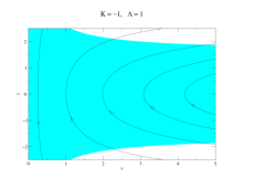
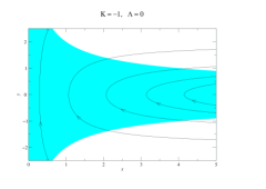
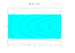
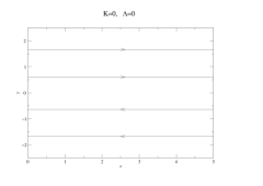
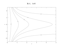
Figure 1: The phase portrait for system (57)–(58) for $n=-2$. For the cases ($K=-1,\Lambda=1$), ($K=-1,\Lambda=0$), ($K=0,\Lambda=1$) the qualitative structure of the phase space is the same. In the finite domains of phase space there are no critical points. Typical trajectories represent the solution starting from singularity-free stage $x=\infty$ at $t=0$, then reach the stage $x=x_{0},y=0$ and goes to infinity. In this three cases the trajectories pass through the acceleration region (the shaded region). The largest acceleration region is for the ($K=-1,\Lambda=1$). These models accelerate for finite interval of time, and this acceleration happens to the models without the cosmological constant. The closed models for ($K=1,\Lambda=0$) are the typical oscillating models. There are no acceleration for ($K=1,\Lambda=0$), ($K=0,\Lambda=0$). In the case of ($K=1,\Lambda=1$) the saddle appears and we have two additional types of evolution. The Lemaître model with quasi-static stage of evolution and models realized in the aforementioned opened and flat models. The acceleration region is in the middle of quasi-static phase of evolution of the Lemaître.

In the projective coordinates $(z,u)$ the above system takes the form

$$\dot{z} =-zu$$ (59)

$$\dot{u} =-2\left(Kz-\frac{2}{3}\Lambda\right)c_{0}^{2}z^{-n}-u^{2}$$ (60)

This form of the system is useful in analysis of behaviour of trajectories at infinity, because $z=0$ corresponds a circle at infinity $x=\infty$ which bounds the phase plane. The phase portraits of system (59)-(60) for $n=-2$ are presented on Fig. 1

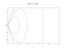
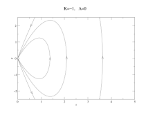
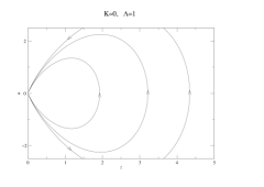
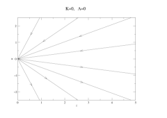
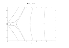
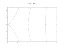
Figure 2: The phase portrait for system (59)–(60) for $n=-2$ in the projective coordinates $z=1/x$, $u=y/x$. All critical points at infinity corresponds to $z_{0}=0$. There are two types of critical points $(z_{0},u_{0})=(0,0)$ or $(z_{0},u_{0})=(2\Lambda/3K,0)$. For all points $\mathop{\mathrm{tr}}A=0$ (where $A$ is a linearization matrix of the considered system), i.e., at least one of the eigenvalues is zero. If ($\Lambda>0$, $K=1$) we have a saddle point at $(z_{0},0)$. The presence of degenerate points at infinity $(0,0)$ that the system is structurally unstable in contrast to the models with positive cosmological constant and constant velocity of light where $(0,\sqrt{4\Lambda/3})$ represents a stable node (the de Sitter stage). For $n>0$ there is no critical points at $(0,0)$ and models are structurally stable.

In this case first integral (28) takes the form

$$\frac{\dot{x}^{2}}{2}+2\int\left(K-\frac{2}{3}\Lambda x\right)c^{2}(x)dx=\bar{C}=\text{const}.$$ (61)

Let us note that in the special cases of $n=-1$ and $n=-2$ the potential takes the particular form $V(x)=2(K\ln x-\frac{2}{3}\Lambda x)$, $V(x)=2(-\frac{K}{x}-\frac{2}{3}\Lambda\ln x)$.

It is clear that first integral (61) is in fact the integral of energy because system (57)–(58) is a Hamiltonian dynamical system with the Hamiltonian

$${\cal H}(p,x)=\frac{p^{2}}{2}+2\left(\frac{Kx^{n+1}}{n+1}-\frac{2}{3}\Lambda\frac{x^{n+2}}{n+2}\right)\equiv\bar{C}=\text{const}>0.$$

Now the integral of energy can be used in the classification of all possible evolution modulo their quantitative (i.e., in accuracy to differential type) properties.

In the qualitative classification, for any case of $\gamma(a)$, first integral (28) may be useful as in the method of the classification previously used in Szydłowski et al. (1984). It assumes the form

$$\frac{p^{2}}{2}+V(a(x))=V(a_{0})$$ (62)

where

$$V(a)=\int^{a(x)}\frac{a^{2}}{\alpha a+1}\left[\frac{K(1+3\gamma(a))}{2a}-\Lambda a\left(1+\frac{1}{3(\alpha a+1)}\right)\right]c^{2}(a)da,$$

$V(a_{0})=\text{const}>0$ and $x=\frac{2\sqrt{2}}{\alpha^{2}}t^{2}(t-1)$, $t=\sqrt{\alpha a+1}$ and $x=a^{2}$ for $\alpha=0$.

From equation (62), after imposing the condition $p=0$, we can calculate $\Lambda$ from the expression on function $\Lambda(a)$ which constitutes a boundary of a domain of configuration space admissible for motion

$$p^{2}\geq 0\quad\Leftrightarrow\quad V(a)-V(a_{0})<0$$

and

$$\Lambda(a)\geq\frac{\int^{a}\frac{a(\alpha a+2)}{2(\alpha a+1)^{2}}Kc^{2}(a)da-V(a_{0})}{\int^{a}\frac{(3\alpha a+4)a^{2}}{3(\alpha a+1)^{2}}c^{2}(a)da}.$$ (63)

By consideration the boundary $\partial D\colon\{(a,\Lambda)\colon\Lambda(a)=0\}$ and construction of the levels $\Lambda=\text{const}$ we obtain the qualitative classification of all possible trajectories in the space $(\Lambda,a)$ or $(\Lambda,x)$.

V.2 How to interpret the acceleration of scale factors and the absence of particle horizon

A great advantage of the phase-space dynamical description is the ability to discuss the distribution of models with given properties. In the other words one can imagine an ansamble of models starting from different initial conditions and ask how a given property is distributed in the ansamble. Now we formulate sufficient conditions for solving the flatness and horizon problems in terms of phase-space relations. Let us recall that the flatness problem is solved whenever the scale factor’s acceleration is positive

$$\ddot{a}(t)>0.$$

This condition is fulfilled in the subspace ${\cal D}_{\text{flat}}$ of the phase space

$${\cal D}_{\text{accel}}=\left\{(a,\dot{a})\colon-\frac{\alpha a+2}{2a(\alpha a+1)}p^{2}-\left(\frac{K(\alpha a+2)}{2a(\alpha a+1)}-\frac{3\alpha a+4}{6(\alpha a+1)}\Lambda a\right)c^{2}(a)>0\right\}.$$ (64)

It means that trajectories representing the histories of VSL universes undergo an accelerated expansion while staying in region ${\cal D}_{\text{flat}}$. One can restate relation (64) using the Hamiltonian constraint $p^{2}=2(V(a_{0})-V(a))$. It is easy to see that the respective condition expressed purely in terms of configuration space, reads

$${\cal D}_{\text{accel}}=\left\{a\colon-\frac{\alpha a+2}{a(\alpha a+1)}(V(a_{0})-V(a))-\left(\frac{K(\alpha a+2)}{2a(\alpha a+1)}-\frac{3\alpha a+4}{6(\alpha a+1)}\Lambda a\right)c^{2}(a)>0\right\}.$$ (65)

Analogous criteria of acceleration if dynamics is covered by equations (47)–(48) are given by (50) in phase space and (52) in the configuration space.

Another interesting question concerns the horizon problems. It is easy to prove the following criterion of avoiding the horizon problem.

Theorem 1

The FRW cosmological model does not have an event horizon near the singularity if $\dot{a}(t)c^{-1}(t)$ tends to a constant while $a(t)$ tends to zero.

Proof. When all events whose coordinates at past time are located beyond some distance $d_{H}$ they can never communicate with the observer at coordinate $r=0$ in the Robertson-Walker metric we can define the distance $d_{H}$ as past event horizon distance. It is given by

$$d_{H}(t)=a(t)\int_{0}^{t_{0}}\frac{dt^{\prime}c(t^{\prime})}{a(t^{\prime})}=a(t)I.$$

Whenever $I$ diverges as $t\to 0$ there is no past event horizon in the space time geometry. On the other hand, when $I$ converges the space time exhibits a past horizon

$$\int_{t}^{t_{0}}\frac{dtc(t)}{a(t)}=\int_{t}^{t_{0}}\frac{a^{n}da}{a\frac{da}{dt}}=\int_{t}^{t_{0}}\frac{1}{c^{-1}\dot{a}}\frac{da}{a}.$$

Let $c^{-1}(t)\dot{a}<A$ then

$$I\geq\frac{1}{A}\int_{0}^{a_{0}}\frac{da}{a}=\frac{1}{A}(\ln a_{0}+\infty).$$

On the other hand when $\dot{a}<\bar{A}$ is bounded then

$$I=\int_{t}^{t_{0}}\frac{dtc(t)}{a(t)}=\int_{t}^{t_{0}}\frac{a^{n}da}{a\frac{da}{dt}}=\int_{t}^{t_{0}}a^{n-1}\frac{da}{\dot{a}}$$

and $I\geq\frac{1}{\bar{A}}\int_{0}^{a_{0}}a^{n-1}da$ or

$$\bar{A}\int_{t}^{t_{0}}\frac{dtc(t)}{\dot{a}(t)}\geq\frac{a^{n}}{n}.$$

Therefore $I$ diverges as $a\to 0$ if $n<0$ and $\dot{a}<\bar{A}$ $\Box$.

The above criterion can be reformulated in the language of the phase space in the form

$$a\to 0\text{ and }c^{-1}(t)\dot{a}(t)\to\text{const},\quad\text{i.e. }a^{-2n}\left(\frac{da}{dt}\right)^{2}\to(\text{const})^{2}.$$

For example for the radiation case $a=\sqrt{x}$ and then the past horizon is eliminated if only $\dot{x}^{2}x^{-2n-1}\to\text{const}$ as $x\to 0$. After substituting first integral (61) we obtain that there is such $n$ that the horizon disappears if only if $n<-1$. Let us note that the above proof is based on the Hamiltonian constraint and is independent of any specific assumption about an equation of state or $a(t)$ near the singuarity. If we assume the power-law behaviour of $a(t)$ then Barrow’s result can be simply achieved Barrow (2002), namely $a(t)\propto t^{2/3(\gamma-1)}$ and if $2\geq 2n+3(\gamma+1)$.

V.3 The potential function for mixture of dust and radiation

The boundary of the domain in the configuration space ($x$-space or $a$-space) admissible for motion is determined by expression for

$$V(a(x))=Kc_{0}^{2}\int^{a(x)}\frac{a^{1+2n}(\alpha a+2)}{(\alpha a+1)^{2}}da-\Lambda c_{0}^{2}\int^{a(x)}\frac{(3\alpha a+4)a^{3+2n}}{3(\alpha a+1)^{2}}da=V(a_{0})>0.$$

The equation $V(a(x))-V(a_{0}(x_{0}))=0$ can be represented in the space $(\Lambda,a)$ or more correctly in the space $(\Lambda,x)$ as a boundary curve for the classification. Instead of the inverse function $a(x)$ (it is difficult to give it in a simple form), we take the function $x(a)$ as

$$V(a_{0})-Kc_{0}^{2}\int^{a}\frac{a^{1+2a}}{2(\alpha a+1)}da-Kc_{0}^{2}\int^{a}\frac{a^{1+2n}}{2(\alpha a+1)^{2}}da+\Lambda c_{0}^{2}\left[\int^{a}\frac{a^{3+2n}}{3(\alpha a+1)}da+\frac{1}{3}\int^{a}\frac{a^{3+2n}}{(\alpha a+1)^{2}}da\right]=0$$

where the physical domain is $V(a_{0})-V(a)>0$, i.e.

$$\Lambda\geq\frac{-V(a_{0})+\frac{1}{2}Kc_{0}^{2}\int^{a}\frac{a^{1+2n}}{\alpha a+1}da+\frac{1}{2}Kc_{0}^{2}\int^{a}\frac{a^{1+2n}}{(\alpha a+1)^{2}}da}{c_{0}^{2}\left[\int^{a}\frac{a^{3+2n}}{3(\alpha a+1)}da+\frac{1}{3}\int^{a}\frac{a^{3+2n}}{(\alpha a+1)^{2}}da\right]}.$$

where

$$\int\frac{da}{a^{m}(\alpha a+1)} = \sum_{k=1}^{m-1}\frac{(-1)^{k}\alpha^{k-1}}{(m-k)!a^{m-k}}+(-1)^{m}\alpha^{m-1}\ln\frac{\alpha a+1}{a}$$

$$\int\frac{da}{a^{l}(\alpha a+1)^{2}} = -\frac{1}{\alpha}\left[\frac{1}{a^{l}(\alpha a+1)}+l\left(\sum_{k=1}^{l}\frac{(-1)^{k}\alpha^{k-1}}{(l+1-k)!a^{l+1-k}}+(-1)^{l+1}\alpha^{l}\ln\frac{\alpha a+1}{a}\right)\right].$$

On the figures 3–5, for the simplicity of presentation without loss of generality, it is assumed $c_{0}=1$, $V(a_{0})=1$ and $K$, $\alpha$ are parameters and $n$ is chosen $-1$, $-2$, $-3$.

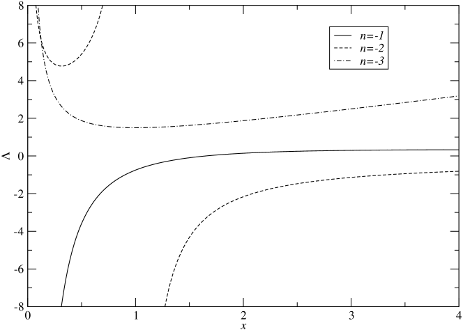
Figure 3: The relationship between $\Lambda$ and $x$ for $K=1$. The qualitative evolution of the models is represented by levels of $\Lambda=\text{const}$. The domain under the characteristic curves $\Lambda(a)$ is classically forbidden. For $n=-1$ and $\Lambda>0$ all models start from finite size of scale factor and expand. For $n=-1$ and $\Lambda>0$ all models start from the singularity and expand. For $n=-2$ and $\Lambda>0$ all models start from finite scale factor and expand. For $n=-2$ and $\Lambda$ there are oscillating universes and with a singularity and other universes expanding from finite scale factor. For $n=-3$ all models are oscillating and with a singularity.

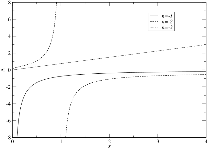
Figure 4: The relationship between $\Lambda$ and $x$ for $K=0$. The qualitative evolution of the models is represented by levels of $\Lambda=\text{const}$. The domain under the characteristic curves $\Lambda(a)$ is classically forbidden. For $n=-1$ and $\Lambda<0$ all models oscillate. For $n=-1$ and $\Lambda>0$ models evolve from a singularity to infinity. For $n=-2$ and $\Lambda<0$ models oscillate. For $n=-2$ and $\Lambda>0$ models also oscillate but without a singularity. For $n=-3$ and $\Lambda<0$ models expand from a singularity to infinity. For $n=-3$ and $\Lambda>0$ all models oscillate.

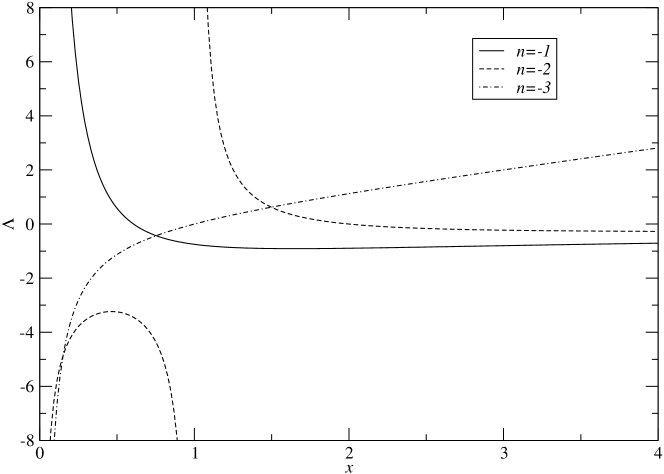
Figure 5: The relationship between $\Lambda$ and $x$ for $K=-1$. The qualitative evolution of the models is represented by levels of $\Lambda=\text{const}$. The domain under the characteristic curves $\Lambda(a)$ is classically forbidden. For $n=-1$ and $\Lambda<0$ there is no solution. For $n=-1$ and $\Lambda>0$ models start from finite size and expand. For $n=-2$ there is discontinuity at $x=1$ and for $\Lambda<0$ some models oscillate from a singularity and other models oscillate without a singularity. For $n=-2$ and $\Lambda>0$ models start from finite size of scale factor to $x=\infty$. For $n=-3$ all models oscillate with a singularity.

VI Tunnelling in $n$ decaying cosmologies

In the classical VSL cosmology a particle trajectory is determined through a knowledge of both a position $x$ and a canonically conjugate momentum $p_{x}$. In the quantum VSL cosmology the notion of trajectories loses its classical meaning due to the uncertainty relation ($x$ and $p_{x}$ are replaced by non-commuting operators). The Wheeler-De Witt equation

$$\left[\frac{\partial^{2}\phantom{x}}{\partial x^{2}}-V(x)\right]\psi(a)=0$$ (66)

is identical to the one-dimensional time-independent Schrödinger equation for a one half unit particle of energy $E$ subject to the potential $V(x)$ ($\psi(a)$ is known as the wave function of the universe).

The ‘particle-universe’ can quantum-mechanically tunnel through the potential barrier. Let us consider the case when the region beneath the barrier $0<a<a_{0}$, is classically forbidden whereas the region $a\geq a_{0}$ is classically allowed.

We can adopt a simple method of calculating an amplitude for the quantum creation of the VSL FRW universe from a zero size to $a=a_{0}=\sqrt{\frac{3(n+2)}{2(n+1)\Lambda}}$

$$|\text{VSLFRW}(a_{0})|\text{nothing}\rangle|^{2}=P\cong\exp\left[-\frac{2}{\hbar}\int_{0}^{x_{0}}\sqrt{2(E-V)}dx\right].$$ (67)

The above formula (called Gamov’s formula) gives us tunnelling probability because the quantized VSL FRW universe is mathematically equivalent to a one-dimensional particle of unit mass.

As an example, let us get back to the previously considered case of the compact vacuum VSL model. The Hamiltonian for this case can be obtained if we put $E=0$ into $\mathcal{H}(p,x)$.

The region of barrier $0<x<x_{0}$ is classically forbidden for the zero energy particle. Therefore one can find the probability that particle at $x=0$ can tunnel to $x=x_{0}\colon V(x_{0})=0$; $x_{0}=\frac{3(n+2)}{2(n+1)\Lambda}$.

After rescaling the variable $x\mapsto x/x_{0}=\kappa$ we obtain for (67)

$$P\cong\exp\left[-\frac{4}{\hbar}\left(\frac{3(n+2)K}{2(n+1)\Lambda}\right)^{(n+3)/2}\right]\int_{0}^{1}\kappa^{n/2}\sqrt{\kappa(1-\kappa)}d\kappa$$ (68)

where we assume $K=1$, $\Lambda\geq 0$ and $-1<n<0$; the potential $V(x)=x^{n+1}(1+x)$ has two extrema and two zeroes. Relation (68) can be rewritten to the form

$$P\cong\exp\left[-\frac{2}{\hbar}F(n)\right]$$ (69)

where

$$F(n)=\left[\frac{3(n+2)}{2(n+1)\Lambda}\right]^{\frac{n+3}{2}}\frac{\sqrt{\pi}}{2}\frac{\Gamma\left(\frac{n+3}{2}\right)}{\Gamma\left(3+\frac{n}{2}\right)}.$$ (70)

It is the most probable that the closed and vacuum VSL FRW model with $-1<n<0$ is born when we have maximum permissible energy density or least size $a_{0}$. It occurs that the creation of the universe with constant $c$ ($n=0$) is the most probable when classical spacetime emerges via the quantum tunnelling process whereas $c(a)$ is a decreasing function during the evolution of the universe.

VII Conclusions

Let us assume that one takes the idea of the varying speed of light seriously as a physical effect that might have happened in the very early universe and today is confined to a very narrow range admissible by inaccuracy of existing bounds on variability of $c$. One of the problems arising then is to see how this modification of physics would change the evolution of standard Friedmann-Robertson-Walker cosmological models. So far only specific qualitative results are known concerning the solution of flatness and horizon problems in VSL models. In the present work we attempted to extend this qualitative discussion in the sense that by constructing phase space portraits of VSL cosmological models we were able to obtain a global view of their dynamics. In order to achieve this we have used a power law Ansatz for function $c(t)$ and investigated classical Einstein equations with $c$ allowed to be a function of time.

The two procedure of reduction of dynamics are proposed. In the first case we reduced the dynamics of VSL models to a two-dimensional Hamiltonian dynamical system with a quadratic kinetic energy form and a potential function depending on a generalized scale factor. In the second one we reparametrized the time variable but the scale factor remains a state variable. In both cases the shape of the potential and the existence of the energy integral was used to classify possible evolutions of VSL models. These possibilities comprise models evolving from the singularity to infinity, oscillatory behaviour between initial and final singularity, Einstein-de Sitter type models evolving from the singularity to the static world, Lemaître-Eddington type models evolving from the static Einstein solution to infinity, models expanding to infinity from the finite size and finally models starting and ending with finite scale factors.

We have dealed with the full global dynamics of VSL models. From the theoretical point of view it is important how large the class of models without horizon or with solved cosmological puzzles is. We call this class of models generic if its inset in the open phase is open or non-zero measure. Such a point of view is justified by the fact that if the solution of a cosmological puzzle is an attribute of a trajectory with a given initial conditions, it should also be an attribute of another trajectory which starts with neighbouring initial conditions.

We have shown that the assumed time dependence of the speed of light leads to a uniform evolution pattern of VSL models on the phase space. The criteria for solving the flatness and horizon problems were formulated in terms of the phase space. It is an advantage of the phase space approach that one can trace the patterns of evolution for all possible initial conditions. We have depicted, on respective phase portraits, the regions where the flatness problem is solved. The models where the region of initial conditions leading to flatness and horizon problem avoidance is large play a distinguished role. From this perspective open ($K=-1$) models with positive cosmological constant $\Lambda>0$ are preferred in the class of VSL FRW models filled with radiation.

The formalism presented in this paper can be easily extended to the case where the matter content of the model is a mixture of different types of matter and to the case of models with shear (e.g. Bianchi I or V).

This formalism can be also treated as a starting point of an application of quantum cosmology to the description of early stages of evolution of the Universe Vilenkin (1982, 1983). The tunnelling rate, with an exact prefactor can be calculated to the first order on $\hbar$ for the closed VSL FRW model with a decaying variable velocity of light term $c(a)$ The tunnelling probability $P$ can be calculated in the WKB approximation given in the $V\gg E$ limit by (67). We consider the closed vacuum VSL FRW models for which potential is qualitatively classical. This implies that $-1<n$. In the interval $-1<n\leq 0$ the probability of tunnelling increases as $F(n)$ monotonically decreases with increasing $n$. It is shown that the highest tunnelling rate occurs for $n=0$; it corresponds to the standard FRW model.

In our work we showed the effectiveness of dynamical system methods in the investigation of VSL FRW models, namely

In the distinguished class of open models with the cosmological constant the acceleration has ‘transitional’ character, i.e., there is a finite time when trajectories are in the acceleration region, and the measure of this region normalized to the area of phase plane is finite, even in the case of $\Lambda=0$.

We can argue that the considered VSL models are structurally unstable (Fig. 2) because of the presence of degenerate critical points at infinity for $n<0$. From the theoretical point of view such a situation seems to be unsatisfactory because in the space of all dynamics systems on the plane they form set of zero measure (the Peixoto theorem).

The advantage of representing dynamics in terms of Hamiltonian is to discuss how trajectories with interesting properties are distributed on phase plane.