Complex Kerr Geometry and Nonstationary Kerr Solutions

Abstract

In the frame of the Kerr-Schild approach, we consider complex structure of the Kerr geometry which is determined by a complex world line of a complex source. The real Kerr geometry is represented as a real slice of this complex structure. The Kerr geometry is generalized to the nonstationary case when the current geometry is determined by a retarded time and is defined by a retarded-time construction via a given complex world line of source. A general exact solution corresponding to arbitrary motion of a spinning source is obtained. The acceleration of the source is accompanied by a lightlike radiation along the principal null congruence. It generalizes to the rotating case the known Kinnersley class of ”photon rocket” solutions.

PACS number(s): 04.20.Jb 04.20.-q 97.60.Lf 11.27.+d

I Introduction

The complex representation of Kerr geometry, initiated by Newman [1], has been found to be useful in various problems [2, 3, 4, 5]. When considered in the Newman-Penrose formalism [6, 7], it allows one to get a retarded-time description of the nonstationary Maxwell fields and twisting algebraically special solutions of the linearized Einstein equations. Twisting solutions are represented in this approach as retarded-time fields, which are similar to Lienard-Wiechard fields. However, they are generated by a complex source moving along a complex world line $x_{0}(\tau)$ in complex Minkowski space-time $CM^{4}$. The light cones emanating from the word line of a source usually play a central role in the retarded-time constructions where the fields are defined by the values of a retarded time. In the case of complex world line, the corresponding light cone has to be complex which complicates the retarded-time scheme.

In this paper, we use the Kerr-Schild approach to the complex representation of Kerr geometry, which is based on the Kerr-Schild formalism and the Kerr theorem[8]. This approach has an advantage in this problem since the Kerr-Schild form of metrics, $g^{\mu\nu}=\eta^{\mu\nu}-2hk^{\mu}k^{\nu}$, contains the auxiliary Minkowski background $\eta^{\mu\nu}$, which attaches an exact meaning to the complex world line $x_{0}(\tau)\in CM^{4}$ in the curved Kerr-Schild backgrounds. In addition, the Kerr theorem allows us to get an explicit representation for the metric, the principal null congruence (PNC), formed by vector field $k^{\mu}$, and the location of singularity and also to express them in asymptotically flat Cartesian coordinates.

This approach allows us to get a class of the exact nonstationary generalizations of the Kerr solution which are determined by the complex retarded-time construction.

The basic ideas of this approach were published in [9, 10, 11, 5]. In [5] this retarded-time construction was applied to describe the boosted Kerr solution. However, application of this approach to accelerating twisting sources encounters hard obstacles connected with the problem of a real slice. In this paper we find the way to solve this problem and present the class of exact nonstationary Kerr solutions.

For the non-rotating sources, such solutions were obtained earlier by Kinnersley [12]. The Kinnersley solutions are radiative, and by acceleration of the source they are accompanied by null radiation. This property is present in our solutions also and leads to the necessity of giving an interpretation to the origin of this radiation, which enforces to return to the old problem of the source of the Kerr and Kerr-Newman solutions.

The main peculiarity of the Kerr geometry is the twisting geodesic and shear-free PNC. Such congruences are determined in Minkowski space-time (parametrized by the null Cartesian coordinates $u,v,\zeta,{\bar{\zeta}}$) by the Kerr theorem [7, 13, 14, 15] via the solution $Y(x)$ of the equation $F=0$, where $F(Y,\lambda_{1},\lambda_{2})$ is an arbitrary analytic function of the projective twistor variables

$$Y,\qquad\lambda_{1}=\zeta-Yv,\qquad\lambda_{2}=u+Y{\bar{\zeta}}.$$ (1)

In twistor notations [14] these variables are defined as follows $\{1,\ Y,\ \lambda_{1},\ \lambda_{2}\}=Z^{\alpha}/Z^{0}$, where $Z^{\alpha}=\{\mu^{A},\quad x^{\nu}\sigma_{\nu\dot{B}B}\mu^{B}\}$. One sees that $Y$ is the ratio of two components of a spinor corresponding to the null direction which is tangent to a null ray of the PNC, while the coordinates $\{\lambda_{1},\ \lambda_{2}\}$ are connected with a shift of this ray from the origin and can be determined by any point $x^{\nu}$ lying on this ray. Therefore, these coordinates fix the position and direction of a null ray in Minkowski space $M^{4}$, in accordance with geometrical meaning of a null twistor, and the scalar function $Y(x)$ determines the null congruence as a field of null directions in $M^{4}$. The geometrical meaning of the twistor coordinates is extended to $CM^{4}$, where they fix complex null planes, and the real null rays of congruence belong to the intersection of the complex conjugate null planes.

The retarded-time construction is usually based on the space-time links provided by light cones. When considering the complex retarded-time construction, we set up a link between the generating PNC function $F$ and the world line of a complex source. In the problem considered there appears the obstacle that the real light cone does not have intersections with complex world line. In $CM^{4}$ light cones split on the families of ‘left’ and ‘right’ complex null planes, which take over the role of the light cone in the complex retarded-time scheme. Each of the ‘left’ null planes is determined by the fixed values of the coordinates $\{Y,\ \lambda_{1},\ \lambda_{2}\}$ and represents a geometrical realization of the twistor [14].

In Sec.II we recollect the basic properties of Kerr geometry and give a nonformal treatment clarifying its complex structure. A consequent treatment based on the Kerr-Schild formalism is started in Sec.III.

In Appendix A we give the basic necessary relations of the Kerr-Schild formalism, and in the Appendix B we give a proof of the Kerr theorem adapted to the Kerr-Schild formalism. During the proof we obtain some relations that are necessary for subsequent treatment of the real slice procedure described in Sec.III. It allows us to integrate the Einstein field equations, which is performed in Sec.IV.

II Complex structure of Kerr geometry and related retarded-time construction

A Appel source and main peculiarities of the real and complex Kerr geometry

The Kerr singular ring is one of the most remarkable peculiarities of the Kerr solution. It is a branch line of space on two sheets: ”negative” and ”positive” where the fields change their signs and directions. There exist the Newton and Coulomb analogues of the Kerr solution possessing the Kerr singular ring. This allows one to understand the origin of this ring as well as the complex origin of the Kerr source. The corresponding Coulomb solution was obtained by Appel still in 1887 by a method of complex shift [17].

A point-like charge $e$, placed on the complex z-axis $(x_{0},y_{0},z_{0})=(0,0,ia)$, gives the real Appel potential

$$\phi_{a}=Re\ e/{\tilde{r}}.$$ (2)

Here $\tilde{r}$ is in fact the Kerr complex radial coordinate $\tilde{r}=PZ^{-1}=r+ia\cos\theta$, where $r$ and $\theta$ are the oblate spheroidal coordinates. It may be expressed in the usual rectangular Cartesian coordinates $x,y,z,t$ as

$$\tilde{r}=[(x-x_{0})^{2}+(y-y_{0})^{2}+(z-z_{0})^{2}]^{1/2}=[x^{2}+y^{2}+(z-ia)^{2}]^{1/2}.$$ (3)

The singular line of the solution corresponds to $r=\cos\theta=0$, and it is seen that the Appel potential $\phi_{a}$ is singular at the ring $z=0,\quad x^{2}+y^{2}=a^{2}$. It was shown that this ring is a branch line of space-time for two sheets, similar to the properties of the Kerr singular ring. Appel potential describes exactly the e.m. field of the Kerr-Newman solution [18].

If the Appel source is shifted to a complex point of space $(x_{o},y_{o},z_{o})\rightarrow(0,0,ia)$, it can be considered as a mysterious ”particle” propagating along a complex world-line $x_{0}^{\mu}(\tau)$ in $CM^{4}$ and parametrized by a complex time $\tau$. The complex source of the Kerr-Newman solution has just the same origin [1, 3] and can be described by means of a complex retarded-time construction for the Kerr geometry.

The Kerr twisting PNC is the second remarkable structure of the Kerr geometry. It is described by a vector field $k^{\mu}$ which determines the Kerr-Schild ansatz for the metric,

$$g_{\mu\nu}=\eta_{\mu\nu}+2hk_{\mu}k_{\nu},$$ (4)

where $\eta_{\mu\nu}$ is an auxiliary Minkowski space-time and

$$h=\frac{mr-e^{2}/2}{r^{2}+a^{2}\cos^{2}\theta}.$$ (5)

This is a remarkable simple form showing that all the complication of the Kerr solution is included in the form of the field $k_{\mu}(x)$ which is tangent to the Kerr PNC. This form shows also that the metric is singular at $r=\cos\theta=0$, which are the focal points of the oblate spheroidal coordinate system.

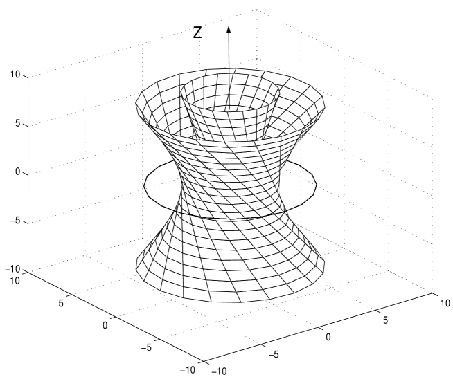
FIG. 1.: The Kerr singular ring and 3D section of the Kerr principal null congruence. Singular ring is a branch line of space, and the PNC propagates from the “negative” sheet of the Kerr space to “positive ” one, covering the space-time twice.

The field $k^{\mu}$ is null with respect to $\eta_{\mu\nu}$ as well as with respect to the metric $g_{\mu\nu}$. The Kerr singular ring and a part of the Kerr PNC are shown in Fig.1. The Kerr PNC consists of the linear generators of the surfaces $\theta=const$. The region shown in Fig.1 $z<0$ corresponds to a “negative” sheet of space ($r<0$) where we set the null rays to be “in”-going.

Twisting vortex of the null rays propagates through the singular ring $r=\cos\theta=0$ and get “out” on the “positive” sheet of space ($z>0$). Indeed, the Kerr congruence covers the space-time twice, and this picture shows only the half of the PNC corresponding to $0>\theta>\pi/2$. It has to be completed by the part for $\pi/2>\theta>\pi$ which is described by another system of the linear generators (having opposite twist). The two PNC directions for each point $x^{\mu}\in M^{4}$ correspond to the known twofoldedness of the Kerr geometry and to the algebraically degenerate metrics of type D.

As it is explicitly seen from the expression for $h$, the Kerr gravitational field has twovaluedness, $h(r)\neq h(-r)$, and so also do the other fields on the Kerr background. The oblate coordinate system turns out to be very useful since it also covers the space twice, for $r>0$ and $r<0$, with the branch line on the Kerr singular ring.

The appearance of the twisting Kerr congruence may be understood as a track of the null planes of the family of complex light cones emanating from the points of the complex world line $x_{0}^{\mu}(\tau)$ [11, 3] in the retarded-time construction. It is very instructive to consider the following splitting of the complex light cones.

B Splitting of the complex light cone

The complex light cone ${\cal K}$ with the vertex at some point $x_{0}$, written in spinor form

$${{\cal K}}=\{x:x=x^{\mu}_{o}(\tau)+\psi^{A}_{L}\sigma^{\mu}_{A\dot{A}}\tilde{\psi}^{\dot{A}}_{R}\}$$ (6)

may be split into two families of null planes: ”left” $(\psi_{L}$ =const; $\tilde{\psi}_{R}$ -variable) and ”right”$(\tilde{\psi}_{R}$ =const; $\psi_{L}$ -variable). These are the only two-dimensional planes that are wholly contained in the complex null cone. The rays of the principal null congruence of the Kerr geometry are the tracks of these complex null planes (right or left) on the real slice of Minkowski space.

The light cone equation in the Kerr-Schild metric coincides with the corresponding equation in Minkowski space because the null directions $k^{\mu}$ are null in both metrics $g_{\mu\nu}$ and $\eta_{\mu\nu}$.

In the null Cartesian coordinates

$$2^{1\over 2}\zeta = x+iy,\qquad 2^{1\over 2}{\bar{\zeta}}=x-iy,$$ (7)

$$2^{1\over 2}u = z+t,\qquad 2^{1\over 2}v=z-t.$$ (8)

the light cone equation has the form $\zeta{\bar{\zeta}}+uv=0$. As usual, in a complex extension to $CM^{4}$ the coordinates $u,v$ have to be considered as complex and coordinates $\zeta$ and ${\bar{\zeta}}$ as independent. On the real section, in $M^{4}$, coordinates $u$ and $v$ take the real values and $\zeta$ and ${\bar{\zeta}}$ are complex conjugate.

The known splitting of the light cone on the complex null planes has a close connection to spinors and twistors. By introducing the projective spinor parameter $Y=\psi^{1}/\psi^{0}$ the equation of complex light cone with the vertex at point $x_{0}$,

$$(\zeta-\zeta_{0})({\bar{\zeta}}-{\bar{\zeta}}_{0})=-(u-u_{0})(v-v_{0}),$$ (9)

splits into two linear equations

$$\zeta-\zeta_{0} = Y(v-v_{0}),$$ (10)

$$-Y({\bar{\zeta}}-{\bar{\zeta}}_{0}) = (u-u_{0})\ ,$$ (11)

describing the ”left” complex null planes (the null rays in the real space). Another splitting

$$-\tilde{Y}(\zeta-\zeta_{0}) = (u-u_{0}),$$ (12)

$$({\bar{\zeta}}-{\bar{\zeta}}_{0}) = \tilde{Y}(v-v_{0})\ ,$$ (13)

gives the ”right” complex null planes.

Thus, the equations of the”left” null planes (11) can be written in terms of the three parameters

$$Y,\qquad\lambda_{1}=\zeta-Yv,\qquad\lambda_{2}=u+Y{\bar{\zeta}},$$ (14)

as follows:

$$\lambda_{1}=\lambda^{0}_{1},\quad\lambda_{2}=\lambda^{0}_{2}\ ,$$ (15)

where

$$\lambda^{0}_{1}=\zeta_{0}-Yv_{0},\qquad\lambda^{0}_{2}=u_{0}+Y{\bar{\zeta}}_{0}$$ (16)

denote the values of these parameters at the point $x_{0}$. These three parameters are the projective twistor variables and very important for further consideration since the Kerr theorem is formulated in terms of these parameters. The above splitting of the complex light cone equation shows their origin explicitly. Note also that in the terms of the Kerr-Schild null tetrad

$$e^{1} = d\zeta-Ydv,\qquad e^{2}=d\bar{\zeta}-\bar{Y}dv,$$ (17)

$$e^{3} = du+\bar{Y}d\zeta+Yd\bar{\zeta}-Y\bar{Y}dv,$$ (18)

$$e^{4} = dv+he^{3},$$ (19)

the projective twistor parameters take the form

$$\lambda_{1} = x^{\mu}e^{1}_{\mu},$$ (20)

$$\lambda_{2} = x^{\mu}(e^{3}_{\mu}-{\bar{Y}}e^{1}_{\mu}),$$ (21)

and correspondingly

$$\lambda^{0}_{1} = x_{0}^{\mu}e^{1}_{\mu},$$ (22)

$$\lambda^{0}_{2} = x_{0}^{\mu}(e^{3}_{\mu}-{\bar{Y}}e^{1}_{\mu}).$$ (23)

The “left” complex null planes of the complex light cone at some point $x_{0}$ can be expressed in terms of the tetrad as follows

$$x_{L}=x_{0}(\tau)+\alpha e^{1}+\beta e^{3}\ ,$$ (24)

and the null plane equations (15) follow then from Eq.(24) and the tetrad scalar products $e^{1\mu}e^{1}_{\mu}=e^{1\mu}e^{3}_{\mu}=e^{3\mu}e^{3}_{\mu}=0$. Similar relations are valid also for the “right” null planes with the replacement $e^{1}\to e^{2}$.

The ”left” null planes of the complex light cones form a complex Kerr congruence which generates all the rays of the principal null congruence on the real space. The ray with polar direction $\theta,\phi$ is the real track of the ”left” plane corresponding to $Y=\exp{i\phi}\tan(\theta/2)$ and belonging to the cone that is placed at the point $x_{0}$ corresponding to $\sigma=a\cos(\theta).$ The parameter $\sigma=Im\tau$ has a meaning only in the range $-a\leq\sigma\leq a$ where the cones have real slices. Thus, the complex world line $x_{0}(t,\sigma)$ represents a restricted two-dimensional surface or strip, in complex Minkowski space, and is really a world-sheet.

The Kerr congruence arises as the real slice of the family of the ”left” null planes ($Y=const.$) of the complex light cones which vertices lie on the complex world line $x_{0}(\tau)$.

The Kerr theorem can be linked to this retarded-time construction.

III Kerr theorem and the retarded-time construction

A The Kerr theorem

Traditional formulation of the Kerr theorem is following.

Any geodesic and shear-free null congruence in Minkowski space is defined by a function $Y(x)$ which is a solution of the equation

$$F=0,$$ (25)

where $F(\lambda_{1},\lambda_{2},Y)$ is an arbitrary analytic function of the projective twistor coordinates

$$Y,\qquad\lambda_{1}=\zeta-Yv,\qquad\lambda_{2}=u+Y{\bar{\zeta}}.$$ (26)

The congruence is determined then by the vector field

$$e^{3}=du+{\bar{Y}}d\zeta+Yd{\bar{\zeta}}-Y{\bar{Y}}dv=Pk_{\mu}dx^{\mu}$$ (27)

in the null Cartesian coordinates $u,\ v,\ {\bar{\zeta}},\ \zeta$.

In the Kerr-Schild backgrounds the Kerr theorem acquires a broader content [8, 9, 11]. It allows one to obtain the position of singular lines, caustics of the PNC, as a solution of the system of equations

$$F=0;\quad dF/dY=0\ ,$$ (28)

and to determine some important parameters of the corresponding solutions:

$$\tilde{r}=-\quad dF/dY,$$ (29)

and

$$P=\partial_{\lambda_{1}}F-{\bar{Y}}\partial_{\lambda_{2}}F.$$ (30)

The parameter $\tilde{r}$ characterizes a complex radial distance, and for the stationary Kerr solution it is a typical complex combination $\tilde{r}=r+ia\cos\theta$. The parameter $P$ is connected with the boost of source.

The proof of the Kerr theorem in the extended version adapted to the Kerr-Schild formalism is given in the Appendix B. Some basic relations of the Kerr-Schild formalism are given in Appendix A.

Working in $CM^{4}$ one has to consider $Y$ and $\bar{Y}$ functionally independent, as well as the null coordinates $\zeta$ and ${\bar{\zeta}}$. The coordinates $u,v$ and congruence turn out to be complex. The corresponding complex null tetrad (123) may be considered as a basis of $CM^{4}$. The Kerr theorem determines in this case only the “left” complex structure - the function $F(Y)$. The real congruence appears as an intersection with a complex conjugate “right” structure.

B Quadratic function F(Y) and interpretation of parameters.

It is instructive to consider first the stationary case. Stationary congruences having Kerr-like singularities contained in a bounded region were considered in papers [27, 10, 16]. It was shown that in this case the function $F$ must be at most quadratic in $Y$,

$$F\equiv a_{0}+a_{1}Y+a_{2}Y^{2}+(qY+c)\lambda_{1}-(pY+\bar{q})\lambda_{2},$$ (31)

where the coefficients $c$ and $p$ are real constants and $a_{0},a_{1},a_{2},q,\bar{q},$ are complex constants. The Killing vector of the solution is determined as

$$\hat{K}=c\partial_{u}+\bar{q}\partial_{\zeta}+q\partial_{\bar{\zeta}}-p\partial_{v}.$$ (32)

Writing the function F in the form

$$F=AY^{2}+BY+C,$$ (33)

one can find two solutions of the equation $F=0$ for the function $Y(x)$

$$Y_{1,2}=(-B\pm\Delta)/2A,$$ (34)

where $\Delta=(B^{2}-4AC)^{1/2}.$

On the other hand from (29)

$$\tilde{r}=-\partial F/\partial Y=-2AY-B,$$ (35)

and consequently

$$\tilde{r}=PZ^{-1}=\mp\Delta.$$ (36)

These two roots reflect the known twofoldedness of the Kerr geometry. They correspond to two different directions of congruence on positive and negative sheets of the Kerr space-time. The expression (30) yields

$$P=pY{\bar{Y}}+\bar{q}{\bar{Y}}+qY+c\ .$$ (37)

C Link to the complex world line of the source.

The stationary and boosted Kerr geometries are described by a straight complex world line with a real 3-velocity $\vec{v}$ in $CM^{4}$:

$$x_{0}^{\mu}(\tau)=x_{0}^{\mu}(0)+\xi^{\mu}\tau;\qquad\xi^{\mu}=(1,\vec{v})\ .$$ (38)

The gauge of the complex parameter $\tau$ is chosen in such a way that $Re\ \tau$ corresponds to the real time $t$.

The function $F$, quadratic in $Y$, can be expressed in this case in the form [27, 10, 11, 5]

$$F\equiv(\lambda_{1}-\lambda_{1}^{0})\hat{K}\lambda_{2}-(\lambda_{2}-\lambda_{2}^{0})\hat{K}\lambda_{1}\ ,$$ (39)

where the twistor components $\lambda_{1},\ \lambda_{2}$ with zero indices denote their values on the points of the complex worldline $x_{0}(\tau)$, Eq.(16), and $\hat{K}$ is a Killing vector of the solution

$$\hat{K}=\partial_{\tau}x_{0}^{\mu}(\tau)\partial_{\mu}=\xi^{\mu}\partial_{\mu}\ .$$ (40)

Application of $\hat{K}$ to $\lambda_{1}$ and $\lambda_{2}$ yields the expressions

$$\hat{K}\lambda_{1} = \partial_{\tau}x_{0}^{\mu}(\tau)e^{1}_{\mu},$$ (41)

$$\hat{K}\lambda_{2} = \partial_{\tau}x_{0}^{\mu}(e^{3}_{\mu}-{\bar{Y}}e^{1}_{\mu}).$$ (42)

From Eq. (30) one obtains in this case

$$P=\hat{K}\rho=\partial_{\tau}x_{0}^{\mu}(\tau)e^{3}_{\mu}\ ,$$ (43)

where

$$\rho=\lambda_{2}+{\bar{Y}}\lambda_{1}=x^{\mu}e^{3}_{\mu}.$$ (44)

Comparing Eqs. (43) and (37) one obtains the correspondence in terms of $\ p,\ c,\ q,\ \bar{q}$,

$$\hat{K}\lambda_{1}=pY+\bar{q},\qquad\hat{K}\lambda_{2}=qY+c,$$ (45)

which allows one to set the relation between the parameters $p,c,q,\bar{q}$, and $\xi^{\mu}$, showing that these parameters are connected with the boost of the source.

The complex initial position of the complex world line $x_{0}^{\mu}(0)$ in Eq. (38) gives six parameters for the solution, which are connected to the coefficients $a_{0},\ a_{1}\ a_{2}\$. It can be decomposed as $\vec{x}_{0}(0)=\vec{c}+i\vec{d}$, where $\vec{c}$ and $\vec{d}$ are real 3-vectors with respect to the space O(3)-rotation. The real part $\vec{c}$ defines the initial position of the source, and the imaginary part $\vec{d}$ defines the value and direction of the angular momentum (or the size and orientation of a singular ring).

It can be easily shown that in the rest frame, when $\vec{v}=0,\quad\vec{d}=\vec{d}_{0}$, the singular ring lies in the orthogonal to $\vec{d}$ plane and has a radius $a=|\vec{d}_{0}|$. The corresponding angular momentum is $\vec{J}=m\vec{d}_{0}.$

D L-projection and complex retarded-time parameter.

In the form (31) all the coefficients are constant while the form (39) has an extra explicit linear dependence on $\tau$ via terms $\lambda_{1}^{0}(x_{0}(\tau))$ and $\lambda_{2}^{0}(x_{0}(\tau))$. However, this dependence is really absent. As a consequence of the relations $\lambda_{1}^{0}(x_{0}(\tau))=\lambda_{1}^{0}(x_{0}(0))+\tau\hat{K}\lambda_{1},\quad\lambda_{2}^{0}(x_{0}(\tau))=\lambda_{2}^{0}(x_{0}(0))+\tau\hat{K}\lambda_{2}$, the terms proportional to $\tau$ cancel and these forms are equivalent.

Parameter $\tau$ may be defined for each point $x$ of the Kerr space-time and plays the role of a complex retarded-time parameter. Its value for a given point $x$ may be defined by L-projection, using the solution $Y(x)$ and forming the twistor parameters $\lambda_{1},\quad\lambda_{2}$ which fix a left null plane.

$L$-projection of the point $x$ on the complex world line $x_{0}(\tau)$ is determined by the condition

$$(\lambda_{1}-\lambda_{1}^{0})|_{L}=0,\qquad(\lambda_{2}-\lambda_{2}^{0})|_{L}=0\ ,$$ (46)

where the sign $|_{L}$ means that the points $x$ and $x_{0}(\tau)$ are synchronized by the left null plane (24),

$$x-x_{0}(\tau_{L})=\alpha e^{1}+\beta e^{3}.$$ (47)

The condition (46) in representation (23) has the form

$$(x^{\mu}-x_{0}^{\mu})e^{1}_{\mu}|_{L}=0,\qquad(x^{\mu}-x_{0}^{\mu})(e^{3}_{\mu}-{\bar{Y}}e^{1}_{\mu})|_{L}=0,$$ (48)

which shows that the points $x^{\mu}$ and $x_{0}^{\mu}$ are connected by the left null plane spanned by the null vectors $e^{1}$ and $e^{3}$.

This left null plane belongs simultaneously to the ”in”-fold of the light cone connected to the point $x$ and to the ”out”-fold of the light cone emanating from a point of the complex world line $x_{0}$. The point of intersection of this plane with the complex world-line $x_{0}(\tau)$ gives the value of the ”left” retarded time $\tau_{L}$, which is in fact a complex scalar function on the (complex) space-time $\tau_{L}(x)$.

By using the null plane equation (46) one can express $\Delta$ of Eq. (36) in the form

$$\Delta|_{L}=(u-u_{0})\dot{v}_{0}+(\zeta-\zeta_{0})\dot{{\bar{\zeta}}_{0}}+({\bar{\zeta}}-{\bar{\zeta}}_{0})\dot{\zeta}_{0}+(v-v_{0})\dot{u}_{0}=\frac{1}{2}\partial_{\tau}(x-x_{0})^{2}=\tau_{L}-t+\vec{v}\vec{R},$$ (49)

where

$$\vec{v}=\dot{\vec{x}_{0}},\qquad\vec{R}=\vec{x}-\vec{x}_{0}.$$ (50)

It gives a retarded-advanced time equation

$$\tau=t\mp\tilde{r}+\vec{v}\vec{R},$$ (51)

and a simple expression for the solutions $Y(x)$:

$$Y_{1}=[(u-u_{0})\dot{v}_{0}+(\zeta-\zeta_{0})\dot{{\bar{\zeta}}}_{0}]/[(v-v_{0})\dot{{\bar{\zeta}}}_{0}-({\bar{\zeta}}-{\bar{\zeta}}_{0})\dot{v}_{0}],$$ (52)

and

$$Y_{2}=[(u-u_{0})\dot{\zeta}_{0}-(\zeta-\zeta_{0})\dot{u}_{0}]/[(u-u_{0})\dot{v}_{0}+(\zeta-\zeta_{0})\dot{{\bar{\zeta}}}_{0}].$$ (53)

For the stationary Kerr solution $\tilde{r}=r+ia\cos\theta$, and one sees that the second root $Y_{2}(x)$ corresponds to a transfer to the negative sheet of the metric: $r\to-r;\quad\vec{R}\to-\vec{R}$, with a simultaneous complex conjugation $ia\to-ia$.

Introducing the corresponding operations,

$$P:r\to-r,\quad\vec{R}\to-\vec{R},$$ (54)

$$C:x_{0}\to\bar{x}_{0},$$ (55)

and also the transfer $"out"\to"in"$

$$T:t-\tau\to\tau-t,$$ (56)

one can see that the roots and corresponding Kerr congruences are CPT-invariant.

E Nonstationary case. Real slice.

In the nonstationary case, this construction acquires new peculiarities.

i/ The coefficients of function $F$ turn out to be complex variables depending on the complex retarded-time parameter;

ii/ $\partial_{\tau}x_{0}^{\mu}=\xi^{\mu}$ can take complex values, which implies complex values for the function $P$ and was an obstacle for obtaining the real solutions in previous investigation [11];

iii/ $K$ is no longer a Killing vector.

To form the real slice of space-time, we have to consider, along with the “left” complex structure generated by a “left” complex world line $x_{0}$, parameter $Y$, and the left null planes, an independent “right” structure with the“right” complex world line $\bar{x}_{0}$, parameter ${\bar{Y}}$, and the right null planes, spanned by $e^{2}$ and $e^{3}$. These structures can be considered as functionally independent in $CM^{4}$, but they have to be complex conjugate on the real slice of space-time.

First, note that for a real point of space-time $x$ and for the corresponding real null direction $e^{3}$, the values of the function

$$\rho(x)=x^{\mu}e^{3}_{\mu}(x)$$ (57)

are real. Next, one can determine the values of $\rho$ at the points of the left and right complex world lines $x_{0}^{\mu}$ and $\bar{x}_{0}^{\mu}$ by L- and R-projections

$$\rho_{L}(x_{0})=x_{0}^{\mu}e^{3}_{\mu}(x)|_{L}$$ (58)

and

$$\rho_{R}(\bar{x}_{0})=\bar{x}_{0}^{\mu}e^{3}_{\mu}(x)|_{R}.$$ (59)

For the ”right” complex structure, the points $x$ and $\bar{x}_{0}(\bar{\tau})$ are to be synchronized by the right null plane $x-\bar{x}_{0}(\bar{\tau}_{R})=\alpha e^{2}+\beta e^{3}$. As a consequence of the conditions $e^{1\mu}e^{3}_{\mu}=e^{3\mu}e^{3}_{\mu}=0$, we obtain

$$\rho_{L}(x_{0})=x_{0}^{\mu}e^{3}_{\mu}(x)|_{L}=\rho(x).$$ (60)

So long as the parameter $\rho(x)$ is real, the parameter $\rho_{L}(x_{0})$ will be real, too. Similarly,

$$\rho_{R}(\bar{x}_{0})={\bar{x}_{0}}^{\mu}e^{3}_{\mu}(x)|_{R}=\rho(x),$$ (61)

and consequently,

$$\rho_{L}(x_{0})=\rho(x)=\rho_{R}(\bar{x}_{0}).$$ (62)

By using Eqs.(23) and (57) one obtains

$$\rho=\lambda_{2}+{\bar{Y}}\lambda_{1}.$$ (63)

Since the L-projection (46) determines the values of the left retarded-time parameter $\tau_{L}=(t_{0}+i\sigma)|_{L}$, the real function $\rho$ acquires an extra dependence on the retarded-time parameter $\tau_{L}$. It should be noted that the real and imaginary parts of $\tau|_{L}$ are not independent because of the constraint caused by L-projection.

It means that the real functions $\rho$ and $\rho_{0}$ turns out to be functions of the real retarded-time parameter $t_{0}=Re\ \tau_{L}$, while $\lambda^{0}_{1}$ and $\lambda^{0}_{2}$ can also depend on $\sigma$.

These parameters are constant on the left null planes, which yields the relations

$$(\sigma|_{L}),_{2}=(\sigma|_{L}),_{4}=0,\quad(t_{0}|_{L}),_{2}=(t_{0}|_{L}),_{4}=0\ .$$ (64)

Similar to the stationary case considered above, we shall restrict function $F$ by the expression quadratic in $Y$

$$F\equiv(\lambda_{1}-\lambda_{1}^{0})K_{2}-(\lambda_{2}-\lambda_{2}^{0})K_{1},$$ (65)

where the functions $K_{1}$ and $K_{2}$ are linear in $Y$ and depend on the retarded-time $t_{0}$. It has to lead to the form (31) with the coefficients depending on the retarded-time.

Let us assumme that the relation $F(Y,t_{0})=0$ holds for the retarded-time evolution $\partial F/\partial{t_{0}}|_{L}=0.$ It yields

$$\frac{\partial F}{\partial{t_{0}}}=K_{1}\partial_{t_{0}}\lambda_{2}^{0}-K_{2}\partial_{t_{0}}\lambda_{1}^{0}+(\lambda_{1}-\lambda_{1}^{0})\partial_{t_{0}}K_{2}-(\lambda_{2}-\lambda_{2}^{0})\partial_{t_{0}}K_{1}=0.$$ (66)

As a consequence of L-projection the last two terms cancel and one obtains

$$({\partial F}/{\partial{t_{0}}})|_{L}=(K_{1}\partial_{t_{0}}\lambda_{2}^{0}-K_{2}\partial_{t_{0}}\lambda_{1}^{0})|_{L}=0,$$ (67)

that is provided by

$$K_{1}(t_{0})=\partial_{t_{0}}\lambda_{1}^{0},\qquad K_{2}(t_{0})=\partial_{t_{0}}\lambda_{2}^{0}\ .$$ (68)

In tetrad representation (23) it takes the form

$$K_{1}=\partial_{t_{0}}x_{0}^{\mu}e^{1}_{\mu},\qquad K_{2}=\partial_{t_{0}}x_{0}^{\mu}(e^{3}_{\mu}-{\bar{Y}}e^{1}_{\mu}).$$ (69)

As a consequence of the relation (30), one obtains

$$P={\bar{Y}}K_{1}+K_{2},$$ (70)

which yields for the function $P$ the real expression

$$P=\partial_{t_{0}}(x_{0}^{\mu}e^{3}_{\mu})|_{L}=\partial_{t_{0}}\rho_{L}\ .$$ (71)

It is seen that $\rho(t_{0})=\rho_{L}(t_{0})$ plays the role of a potential for $P$, similarly to some nonstationary solutions presented in [7].

It seems that the extra dependence of the function $F$ on the nonanalytic retarded-time parameters $t_{0}$ contradicts the Kerr theorem; however, the nonanalytic part disappears and analytic dependence on $Y,\quad l_{1},\quad l_{2}$ is reconstructed by L-projection. This is explicitly seen for the quadratic form (65) with coefficients given by Eq.(68). Indeed, direct differentiation of this form yields the expression

$$dY=ae^{1}+be^{3}+cdt_{0}\ ,$$ (72)

where $c=(\lambda_{1}-\lambda_{1}^{0})\partial_{t_{0}}K_{2}-(\lambda_{2}-\lambda_{2}^{0})\partial_{t_{0}}K_{1}$. By L-projection one has $c|_{L}=0$ and the nonanalytic term $cdt_{0}$ cancels. Therefore, the differential of the function $Y(x)$ by L-projection satisfies the geodesic and shear free conditions (133) provided by the Kerr theorem. Note that all the real retarded-time derivatives on the real space-time are nonanalytic and have to involve the conjugate right complex structure. In particular, the expressions (69) acquire the form

$$K_{1}=e^{1}_{\mu}Re\ \dot{x}_{0}^{\mu},\qquad K_{2}=(e^{3}_{\mu}-{\bar{Y}}e^{1}_{\mu})Re\ \dot{x}_{0}^{\mu},$$ (73)

where $\dot{x}_{0}^{\mu}=\partial_{t_{0}}x_{0}^{\mu}\ .$

IV Solution of the field equations

We are now able to obtain a general class of accelerating radiating solutions representing arbitrary nonstationary generalization of the Kerr solution. For simplicity, we shall assume that there is no electromagnetic field. As in the Kinnersley case, the null radiation is described by an incoherent flow of the lightlike particles in $e^{3}$ direction. The solution of the field equations is similar to the treatment given for the Kerr-Schild form of metric in [8]

In particular, we have

$$R_{24}=R_{22}=R_{44}=0.$$ (74)

If the electromagnetic field is zero we also have

$$R_{12}=R_{34}=0.$$ (75)

The equation

$$h,_{44}+2(Z+{\bar{Z}})h,_{4}+2Z{\bar{Z}}h=0,$$ (76)

which follows from (75), admits the solutions

$$h=M(Z+{\bar{Z}})/2,$$ (77)

where $M$ is a real function, obeying the conditions $M,_{4}=0$.

Next, the equation

$$R_{23}=0,$$ (78)

acquires the form

$$M,_{2}-3Z^{-1}{\bar{Z}}Y,_{3}M=0.$$ (79)

The last gravitational field equation $R_{33}=-P_{33}\equiv-\kappa T_{33}$ takes the form

$${\cal D}M=Z^{-1}{\bar{Z}}^{-1}P_{33}/2,$$ (80)

where

$${\cal D}=\partial_{3}-Z^{-1}Y,_{3}\partial_{1}-{\bar{Z}}^{-1}{\bar{Y}},_{3}\partial_{2}\ ,$$ (81)

which corresponds to the null radiation in the form $\kappa T_{\mu\nu}=P_{33}e^{3}_{\mu}e^{3}_{\nu}$.

To integrate Eq.(79) we use the relation (142) of corollary 1 and obtain the equation

$$(\log MP^{3}),_{2}=0$$ (82)

which has the general solution

$$M=m/P^{3},$$ (83)

where

$$m,_{4}=m,_{2}=0.$$ (84)

On the real slice functions $m$ and $P$ depend on the retarded-time $t_{0}$. The action of operator ${\cal D}$ on the variables $Y,\bar{Y}$ and $\rho$ is

$${\cal D}Y={\cal D}\bar{Y}=0,\qquad{\cal D}\rho=1\ .$$ (85)

From these relations and Eq. (71) we have ${\cal D}\rho=\partial\rho/\partial t_{0}{\cal D}t_{0}=P{\cal D}t_{0}=1$, which yields

$${\cal D}t_{0}=P^{-1}.$$ (86)

Since $M$ is also a function of $Y,\bar{Y}$, and $t_{0}$, the last equation (80) takes the form

$$\partial_{t_{0}}M=PZ^{-1}{\bar{Z}}^{-1}P_{33}/2.$$ (87)

It is not really a field equation but a definition of the stress-energy tensor $\kappa T_{\mu}^{\nu}=P_{33}e^{3}_{\mu}e^{3\nu}$ corresponding to the null radiation. Substituting Eq.(83) one obtains two terms:

$$P_{33}=\frac{1}{P^{2}|\tilde{r}|^{2}}[-6m(\partial_{t_{0}}\log P)+2\partial_{t_{0}}m].$$ (88)

The first term, proportional to $\partial_{t_{0}}\log P$, is connected with the acceleration. The second term, proportional to $\partial_{t_{0}}m$, describes the loss of mass by radiation corresponding to the Vaidia “shining star” solution [7, 22, 23].

The resulting metric has the form

$$g_{\mu\nu}=\eta_{\mu\nu}+(m/P^{3})(Z+\bar{Z})e^{3}_{\mu}e^{3}_{\nu}.$$ (89)

Normalizing $e^{3}$ by introducing $k^{\mu}=e^{3\mu}/P$, one has

$${\dot{x}}_{0}^{\mu}k_{\mu}=1,$$ (90)

and using $\tilde{r}=PZ^{-1}$ we simplify the expressions for metric and stress-energy tensor.

Let us summarize the solutions we have obtained. The metric is

$$g_{\mu\nu}=\eta_{\mu\nu}+m({\tilde{r}}^{-1}+\bar{\tilde{r}}^{-1})k_{\mu}k_{\nu},$$ (91)

and the radiation is

$$\kappa T_{\mu}^{\nu}=\Phi k_{\mu}k^{\nu},$$ (92)

where

$$\Phi=\frac{1}{|\tilde{r}|^{2}}[-6m(\partial_{t_{0}}\log P)+2\partial_{t_{0}}m].$$ (93)

Vector field $k_{\mu}$ is defined by

$$k_{\mu}dx^{\mu}=e^{3}/P=P^{-1}(du+{\bar{Y}}d\zeta+Yd{\bar{\zeta}}-Y{\bar{Y}}dv).$$ (94)

Function $Y(x)$ is given in terms of the coordinates $u,v,\zeta,{\bar{\zeta}}$, by equation $F(Y)=AY^{2}+BY+C=0$, where the coefficients $A,B,C$ are determined by decomposition of function

$$F\equiv(\lambda_{1}-\lambda_{1}^{0})K_{2}-(\lambda_{2}-\lambda_{2}^{0})K_{1},$$ (95)

and $P$ is given by

$$P(t_{0})=K_{2}+{\bar{Y}}K_{1}=e^{3}_{\mu}Re\ \dot{x}_{0}^{\mu}\ ,$$ (96)

where

$$\lambda_{1}=\zeta-Yv,\qquad\lambda_{2}=u+Y{\bar{\zeta}},$$ (97)

and

$$\lambda^{0}_{1}=\zeta_{0}-Yv_{0},\qquad\lambda^{0}_{2}=u_{0}+Y{\bar{\zeta}}_{0}$$ (98)

are the values of these variables on the complex world line, and

$$K_{1}=e^{1}_{\mu}Re\ \dot{x}_{0}^{\mu},\qquad K_{2}=(e^{3}_{\mu}-{\bar{Y}}e^{1}_{\mu})Re\ \dot{x}_{0}^{\mu}.$$ (99)

The complex radial coordinate is given by

$$\tilde{r}=-dF/dY=-2AY-B.$$ (100)

The coefficients $A,B,C$, the functions $K_{1}$ and $K_{2}$ and the parameters of the function $P$ are determined by a given complex world line $x_{0}^{\mu}(\tau)=\{u_{0}(\tau),v_{0}(\tau),\zeta_{0}(\tau),{\bar{\zeta}}_{0}(\tau)\}$ and have a current dependence on the retarded time $\tau|_{L}$ which is determined by L-projection on the given complex world line as a root of the left null plane equation

$$\lambda_{1}=\lambda^{0}_{1}\ ,\quad\lambda_{2}=\lambda^{0}_{2}\ .$$ (101)

Solution of these equations has to be performed for all points of space-time in the region of interest. This is a nonlinear problem with many unknown functions. In the general case it needs a large body of numerical computations with subsequent iterative refinement. For the beginning of the iterative process a starting ‘point’ is necessary, which gives an initial approximation. To obtain it the analytical solutions in the local regions of short distances $|\tilde{r}|\sim|t-\tau|<<\dot{x}_{0}^{\mu}k_{\mu}/\ddot{x}_{0}^{\mu}k_{\mu}$, can be used since all the unknown parameters (for exclusion of radiation) are determined by the first derivative of the complex world line and the nonlinearity caused by acceleration is negligible here. Having at hand the initial field $Y(x)$, one can use the following iterative loop scheme of computation:

$$x\to Y(x)\to\{\lambda_{1},\lambda_{2},\rho\}\to\{\tau,x_{0},\lambda^{0}_{1},\lambda^{0}_{2}\}\to\{P,K_{1},K_{2}\}\to F(Y)\to\{Y(x),e^{3}\}\to cycle\ loop\ .$$ (102)

This iterative procedure is needed to refine the data and carry out a progressive extension of the region. The obtained local parameters $Y,K_{1},K_{2},\lambda^{0}_{1},\lambda^{0}_{2},A,B,C,F,P,\tau|_{L}$ can be immediately extended along the rays of PNC from the short distances to large ones, which allows one to reduce considerably the necessary body of computations.

The following example is instructive since it shows that some of parameters can be determined analytically; however, an essential nonlinearity is retained which demands the numerical computations.

Example

Let us consider circular motion of source in (x,y)-plane with the direction of angular momentum $\vec{J}=m\vec{a}$ along z-axis. This example is interesting for astrophysical applications and as a model of circular motion of polarized spinning particles in accelerators. For the both cases one can assume $|a|<|b|$. The corresponding complex world line will be

$$x^{\mu}_{0}(\tau)=(\tau,\ b\cos\omega t_{0},\ b\sin\omega t_{0},\ ia\ ),\qquad\tau=t_{0}+i\sigma.$$ (103)

In null coordinates $u,v,\zeta,{\bar{\zeta}}$ it takes the form

$$x_{0}(\tau)=2^{-1/2}(ia+\tau,\ ia-\tau,\ be^{i\omega t_{0}},\ be^{-i\omega t_{0}}\ ),$$ (104)

and we have

$$\dot{x}_{0}(\tau)=2^{-1/2}(1,\ -1,\ ib\omega e^{i\omega t_{0}},\ -ib\omega e^{-i\omega t_{0}}\ ).$$ (105)

The expression for $\rho_{0}$ will be

$$\rho_{0}=2^{-1/2}[\tau(1+Y{\bar{Y}})+b({\bar{Y}}e^{i\omega t_{0}}+Ye^{-i\omega t_{0}})+ia(1-Y{\bar{Y}})].$$ (106)

On the left null plane it has to be real that leads to

$$\sigma|_{L}=a(1-Y{\bar{Y}})/(1+Y{\bar{Y}}),$$ (107)

and

$$\rho_{0}|_{L}=2^{-1/2}[t_{0}(1+Y{\bar{Y}})+b({\bar{Y}}e^{i\omega t_{0}}+Ye^{-i\omega t_{0}})],$$ (108)

and yields

$$P=\dot{\rho}_{0}|_{L}=2^{-1/2}(1+Y{\bar{Y}})+i2^{-1/2}\omega b({\bar{Y}}e^{i\omega t_{0}}-Ye^{-i\omega t_{0}}).$$ (109)

One can also obtain

$$\lambda^{0}_{1}=2^{-1/2}[be^{i\omega t_{0}}+Y(\tau_{L}-ia)],\quad\lambda^{0}_{2}=2^{-1/2}[Ybe^{-i\omega t_{0}}+(\tau_{L}+ia)],$$ (110)

and

$$K_{1}=2^{-1/2}[ib\omega e^{i\omega t_{0}}+Y],\quad K_{2}=2^{-1/2}[1-Yib\omega e^{-i\omega t_{0}}].$$ (111)

Coefficients of the function $F=AY^{2}+BY+C$ take the form

$$A=2^{-1/2}\{ib\omega e^{-i\omega t_{0}}[v-2^{-1/2}(ia-\tau_{L})]-[{\bar{\zeta}}-2^{-1/2}be^{-i\omega t_{0}}]\},$$ (112)

$$B=-2^{-1/2}\{ib\omega e^{-i\omega t_{0}}[\zeta-2^{-1/2}be^{-i\omega t_{0}}]+ib\omega e^{i\omega t_{0}}[{\bar{\zeta}}-2^{-1/2}be^{i\omega t_{0}}]+(u+v-2^{1/2}ia)\},$$ (113)

$$C=2^{-1/2}\{-ib\omega e^{i\omega t_{0}}[u-2^{-1/2}(ia+\tau_{L})]+[\zeta-2^{-1/2}be^{i\omega t_{0}}]\}.$$ (114)

However, since these coefficients depend on the parameter $\sigma=Im\ \tau_{L}$, which is determined by L-projection as a function of $Y$, the equation $F=0$ turns out to be nonlinear. The iterative procedure is necessary for its solution. The dependence of $A,B,C$ on $\sigma$ has the factor $b\omega$. The case $b\omega<<1$ corresponds to nonrelativistic motion. The dependence on $\sigma$ is weak when $b\omega<<|Y|\sim 1$, but grows when $b\omega\sim|Y|$ or $b\omega\sim|1/Y|$. Neglecting $\sigma$ in the equation $F=0$, one can obtain the analytical solution $Y(x)$, which can be used as a first approximation. Note also that in the distant zone the role of rotation parameter $a$ becomes weak and the simpler Kinnersley solution can be used for correction of the parameters.

Transfer to the Kinnersley solutions.

For the twist-free, nonrotating Kinnersley’s case the world line is real, $Im\ x_{0}=0$, and the radial distances $\tilde{r}=\bar{\tilde{r}}=r$ and the ‘right’ and ‘left’ retarded-time parameters coincide $\tau_{L}=\tau_{R}=t_{0}$. The retarded-time equation following from Eq.(51) can be represented in the form

$$\tilde{r}=-(t-t_{0})+\vec{v}\vec{R}=(x^{\mu}-x_{0}^{\mu})\dot{x}_{0\mu}.$$ (115)

It turns out to be real, and in the terms of the Kinnersley parameters $\sigma^{\mu}=x^{\mu}-x_{0}^{\mu}$ it yields the relation

$$\tilde{r}=r=\sigma^{\mu}\dot{x}_{0\mu}.$$ (116)

On the other hand, the real null vectors $\sigma^{\mu}=x^{\mu}-x_{0}^{\mu}$ are proportional to $e^{3\mu}$, and taking into account Eq.(96) we have $r=\sigma^{\mu}\dot{x}_{0\mu}=\beta e^{3\mu}\dot{x}_{0\mu}=\beta P$, which yields $\beta=r/P$ and $\sigma^{\mu}=re^{3\mu}/P=rk^{\mu}$. This relation shows that our PNC field $k^{\mu}$ coincides with the Kinnersley definition of the PNC, $k^{\mu}=\sigma^{\mu}/r$, in terms of which

$$\partial_{t_{0}}\log P=\dot{P}/P=\ddot{x}_{0}^{\mu}k_{\mu}\ ,$$ (117)

and the metric (91) and radiation (92), (93) take the Kinnersley form [12]

$$g_{\mu\nu}=\eta_{\mu\nu}+\frac{2m(t_{0})}{r}(\sigma_{\mu}/r)(\sigma_{\nu}/r),$$ (118)

$$\kappa T_{\mu}^{\nu}=\Phi k_{\mu}k^{\nu},\qquad\Phi=\frac{1}{r^{2}}[-6m(\ddot{x}_{0}^{\mu}k_{\mu})+2\dot{m}].$$ (119)

V Conclusion

The complex retarded-time construction considered permits us to obtain a class of nonstationary rotating solutions generated by a complex source moving along an arbitrary given complex world line.

These solutions represent a natural generalization of the Kinnersley class of solutions to the rotating case. The Kerr-Schild approach allows one to get exact expressions for the metric, coordinate system, the PNC, and the positions of singularity for arbitrary motion of a rotating source.

The solutions obtained represent a natural generalization of the black hole solutions, and if $m^{2}<e^{2}+a^{2}$ they have horizons. However, since the solutions are radiative, the usual black-hole interpretation can meet objections, and an additional treatment of this case is necessary, which we intend to do elsewhere. The solutions can find application for modelling the behavior of spinning astrophysical objects by acceleration and relativistic boosts. They are also interesting for investigation of the relativistic gravitational fields by particle scattering in ultrarelativistic regimes [5].

By $a^{2}+e^{2}>m^{2}$ the horizons disappear and there is a naked singular ring. This case has attracted attention as a model of a spinning particle [9, 10, 18, 27, 24, 25, 26]. In [9, 10, 27] the Kerr singular ring was considered as a closed relativistic string forming the source of spinning particle [18]. The nonstationary Kerr solutions presented allows one to describe excitations of this string. In this case, the “negative” sheet of the Kerr space has to be considered as a sheet of advanced fields belonging to the field of vacuum fluctuations, and thus the e.m. radiation must belong to the zero point field. The outgoing vortex of the null radiation appears as a result of the resonance of the vacuum field on this relativistic string. In this case, the energy-momentum tensor has to be regularized on the classical level by the known procedure [28]

$$T_{reg}^{\mu\nu}=\ :T^{\mu\nu}:\ \equiv T^{\mu\nu}-<0|T^{\mu\nu}|0>,$$ (120)

which has to satisfy the condition $\nabla_{\mu}T_{reg}^{\mu\nu}=0$. It corresponds exactly to a subtraction of this radiation, leading to $T_{reg}^{\mu\nu}=0$ [9, 10]. On the quantum level this procedure is equivalent to the postulate on the absence of radiation for oscillating strings. This stringy interpretation of the Kerr source will be considered elsewhere.

The class of solutions presented can easily be generalized to the Kerr-Newman solution and to the sources radiating electrical charges.

Some other known generalizations of the Kerr solution, such as the Kerr-Sen solution to low energy string theory [29], the solution to broken $N=2$ supergravity [4], and regular rotating particlelike objects built on the base of Kerr-Newman solution [30], retain the form and the geodesic and shear-free properties of the Kerr PNC. This means that the Kerr theorem is also valid for these solutions, and that they can also be generalized to the nonstationary radiating case.

Appendix A: Basic relations of the Kerr-Schild formalism

Following the notations of Ref.[8], the Kerr-Schild null tetrad $e^{a}=e^{a}_{\mu}dx^{\mu}$ is determined by the relations

$$e^{1} = d\zeta-Ydv,\qquad e^{2}=d\bar{\zeta}-\bar{Y}dv,$$ (121)

$$e^{3} = du+\bar{Y}d\zeta+Yd\bar{\zeta}-Y\bar{Y}dv,$$ (122)

$$e^{4} = dv+he^{3},$$ (123)

and

$$g_{ab}=e_{a}^{\mu}e_{b\mu}=\left(\begin{array}[]{cccc}0&1&0&0\\ 1&0&0&0\\ 0&0&0&1\\ 0&0&1&0\end{array}\right).$$ (124)

The vectors $e^{3},e^{4}$ are real, and $e^{1},e^{2}$ are complex conjugate.

The Ricci rotation coefficients are given by

$$\Gamma^{a}_{bc}=-\quad e^{a}_{\mu;\nu}e_{b}^{\mu}e_{c}^{\nu}.$$ (125)

The PNC have the $e^{3}$ direction as tangent. It will be geodesic if and only if $\Gamma_{424}=0$ and shear free if and only if $\Gamma_{422}=0$. The corresponding complex conjugate terms are $\Gamma_{414}=0$ and $\Gamma_{411}=0$.

The inverse (dual) tetrad has the form

$$\partial_{1} = \partial_{\zeta}-{\bar{Y}}\partial_{u},$$ (126)

$$\partial_{2} = \partial_{\bar{\zeta}}-Y\partial_{u},$$ (127)

$$\partial_{3} = \partial_{u}-h\partial_{4},$$ (128)

$$\partial_{4} = \partial_{v}+Y\partial_{\zeta}+{\bar{Y}}\partial_{\bar{\zeta}}-Y{\bar{Y}}\partial_{u},$$ (129)

where $\partial_{a}\equiv,_{a}\equiv e_{a}^{\mu}\partial,_{\mu}$.

The parameter $Z=Y,_{1}=\rho+i\omega$ is a complex expansion of the congruence, $\rho=expansion$ and $\omega=rotation$. $Z$ is connected to the complex radial distance $\tilde{r}$ by the relation

$$\tilde{r}=PZ^{-1}.$$ (130)

It was shown in [8] that the connection forms in Kerr-Schild metrics are

$$\Gamma_{42}=\Gamma_{42a}e^{a}=-dY-hY,_{4}e^{4}.$$ (131)

The congruence $e^{3}$ is geodesic if $\Gamma_{424}=-Y,_{4}(1-h)=0,$ and is shear free if $\Gamma_{422}=-Y,_{2}=0.$ Thus, the function $Y(x)$ with the conditions

$$Y,_{2}=Y,_{4}=0$$ (132)

defines a shear-free and geodesic congruence.

Appendix B: Proof of the Kerr Theorem and two corollaries.

The proof given bellow of the Kerr theorem follows to the general scheme sketched in [8].

Proof. The differential of the function $Y$ in the case of $Y,_{2}=Y,_{4}=0$ has the form

$$dY=Y,_{a}e^{a}=Y,_{1}e^{1}+Y,_{3}e^{3}.$$ (133)

As the first step we work out the form of $Y,_{3}$. By using relations (129) and their commutators we find

$$Z,_{2}=(Z-\bar{Z})Y,_{3}.$$ (134)

Straightforward differentiation of $Y,_{3}$ gives the equation

$$Y,_{32}=(Y,_{3})^{2},$$ (135)

and by using Eqs.(134) and (135) we obtain the equation

$$(Z^{-1}Y,_{3}),_{2}=\bar{Z}(Z^{-1}Y,_{3})^{2}.$$ (136)

This is a first-order differential equation for the function $Z^{-1}Y,_{3}$. Its general solution can be obtained by the substitution $x=Z(Y,_{3})^{-1}$ and has the form

$$Y,_{3}=Z(\phi-\bar{Y})^{-1},$$ (137)

where $\phi$ is an arbitrary solution of the equation $\phi,_{2}=0$. Analogously, by using the relation $Y,_{34}=-ZY,_{3}$ one gets $\phi,_{4}=0$; therefore $\phi$ may be an arbitrary function satisfying

$$\phi,_{2}=\phi,_{4}=0.$$ (138)

One can also mention that the three projective twistor coordinates $\lambda_{1}=\zeta-Yv,\qquad\lambda_{2}=u+Y{\bar{\zeta}},$ and $Y$ satisfy similar relations $(.),_{2}=(.),_{4}=0$. Since the surface $\phi=const$ forms a sub-manifolds of $CM^{4}$ that has the complex dimension 3, an arbitrary function $\phi$ satisfying Eq.(138) may be presented as function of three projective twistor coordinates $\phi=\phi(Y,\lambda_{1},\lambda_{2})$. Now we can substitute $Y,_{3}$ in Eq.(133), which implies

$$Z^{-1}({\bar{Y}}-\phi)dY=\phi(d\zeta-Ydv)+(du+Yd{\bar{\zeta}}).$$ (139)

If an arbitrary analytic function $F(Y,\lambda_{1},\lambda_{2})$ is given, then differentiating the equation $F(Y,\lambda_{1},\lambda_{2})=0$ and comparing the result with Eq.(139), we find that

$$PZ^{-1}=-\quad dF/dY,\qquad P=\partial_{\lambda_{1}}F-{\bar{Y}}\partial_{\lambda_{2}}F,$$ (140)

where the function $P$ can also be defined as

$$P=(\phi-\bar{Y})\partial_{\lambda_{2}}F.$$ (141)

Corollary 1. The following useful relations are valid:

$$\bar{Z}Z^{-1}Y,_{3}=-(\log P),_{2}\ ,\quad P,_{4}=0.$$ (142)

Proof. So long as $\partial_{2}\partial_{\lambda_{2}}F=0$, one sees that

$$(\log P),_{2}=-\bar{Z}(\phi-{\bar{Y}})^{-1};$$ (143)

then Eq.(137) leads to first equality of Eq.(142). The relation $P,_{4}=0$ follows from Eq.(140) and the properties of the twistor components $Y,_{4}=(\lambda_{1}),_{4}=(\lambda_{2}),_{4}=0$.

Corollary 2. Singular region of the congruence, where the complex divergence $Z$ blows up, is defined by the system of equations (28).

REFERENCES

- [1] E.T. Newman, J.Math.Phys. 14(1973)102. R.W. Lind, E.T. Newman, J. Math. Phys. 15(1974)1103.
- [2] E.T. Newman, Phys. Rev. D 65 (2002) 104005.
- [3] A.Ya. Burinskii, String-like Structures in Complex Kerr Geometry. In: “Relativity Today”, Edited by R.P.Kerr and Z.Perjés, Akadémiai Kiadó, Budapest, 1994, p.149. Phys.Lett. A 185 (1994) 441.
- [4] A.Ya. Burinskii, Phys.Rev.D 57 (1998)2392. Class. Quant. Grav. 16(1999)3497.
- [5] A.Ya. Burinskii and G. Magli, Annals of the Israel Physical Society, 13 (1997) 296. Phys.Rev.D 61(2000)044017.
- [6] E. Newman and R. Penrose. Journ. Math. Phys. 3 (1962)566.
- [7] D.Kramer, H.Stephani, E. Herlt, M.MacCallum, “Exact Solutions of Einstein’s Field Equations”, Cambridge Univ. Press, Cambridge 1980.
- [8] G.C. Debney, R.P. Kerr, A.Schild, J. Math. Phys. 10(1969) 1842.
- [9] D. Ivanenko and A.Ya. Burinskii, Izvestiya Vuzov Fiz. n.7 (1978) 113 (in Russian).
- [10] A.Ya. Burinskii, Strings in the Kerr-Schild metrics In: “Problems of theory of gravitation and elementary particles”,11(1980)47, Moscow, Atomizdat, (in Russian).
- [11] A. Burinskii, R.P. Kerr and Z. Perjes, in: Abstracts of 14th International Conference on General Relativity and Gravitation (Florence, Italy 1995), p. A71; A. Burinskii and R.P. Kerr “Nonstationary Kerr Congruences”, e-print gr-qc/9501012.
- [12] W. Kinnersley, Phys. Rev. 186 (1969) 1335.
- [13] R. Penrose, J. Math. Phys. 8(1967) 345.
- [14] R. Penrose, W. Rindler, Spinors and space-time.v.2. Cambridge Univ. Press, England, 1986.
- [15] D.Cox and E.J. Flaherty, Commun. Math. Phys. 47(1976)75.
- [16] R.P. Kerr, W.B. Wilson, Gen. Rel. Grav. 10(1979)273.
- [17] E.T. Whittacker and G.N. Watson, “A Course of Modern Analysis”, Cambrige Univ. Press London/New York,p.400, 1969 .
- [18] A.Ya. Burinskii, Sov. Phys. JETP, 39(1974)193.
- [19] H. Ooguri and C. Vafa. Nucl. Phys. B 361(1991)469; B.361(1991)83.
- [20] O. Veblen. Proc. Nat. Acad. Sci. (USA). v.XIX (1933)462.
- [21] H. Ruse. Proc. Roy. Soc. of Edinburg. 37 (1936/37) 97.
- [22] P.C. Vaidya and L.K. Patel. Phys. Rev. D 7(1973)3590.
- [23] V. P. Frolov, V.I. Khlebnikov Gravitational field of radiating systems: I. Twisting free type D metrics. Preprint No.27, Lebedev Fiz. Inst., Akad. Nauk, Moscow, 1975.
- [24] B. Carter, Phys. Rev. 174 (1968) 1559.
- [25] W. Israel, Phys. Rev. D2 (1970) 641.
- [26] C.A. López, Phys. Rev. D30 (1984) 313.
- [27] D. Ivanenko and A.Ya. Burinskii, Izvestiya Vuzov Fiz. n.5 (1975) 135 (in Russian).
- [28] B.S. De Witt, Phys. Reports. C19 (1975) 295.
- [29] A. Sen, Phys. Rev. Lett. 69(1992)1006.
- [30] A. Burinskii, E. Elisalde, S. Hildebrandt and G. Magli. Phys. Rev.D65 (2002)064039.