Renormalization of Discrete Models without Background

Conventional renormalization methods in statistical physics and lattice quantum field theory assume a flat metric background. We outline here a generalization of such methods to models on discretized spaces without metric background. Cellular decompositions play the role of discretizations. The group of scale transformations is replaced by the groupoid of changes of cellular decompositions. We introduce cellular moves which generate this groupoid and allow to define a renormalization groupoid flow.

We proceed to test our approach on several models. Quantum BF theory is the simplest example as it is almost topological and the renormalization almost trivial. More interesting is generalized lattice gauge theory for which a qualitative picture of the renormalization groupoid flow can be given. This is confirmed by the exact renormalization in dimension two.

A main motivation for our approach are discrete models of quantum gravity. We investigate both the Reisenberger and the Barrett-Crane spin foam model in view of their amenability to a renormalization treatment. In the second case a lack of tunable local parameters prompts us to introduce a new model. For the Reisenberger and the new model we discuss qualitative aspects of the renormalization groupoid flow. In both cases quantum BF theory is the UV fixed point.

1 Introduction

Renormalization is an essential tool both in condensed matter and high energy physics. It is necessary to make sense of and understand the properties of physical models. In the first case and to some extent also in the second, models are often defined as state sums on discretizations of space-time (spin systems, lattice gauge theory etc.). Renormalization consists then in understanding and controlling the behaviour of a model under changes of the discretization.

The discretizations of space (or space-time) employed in these models are usually hyper-cubic or other types of regular lattices. This is justified by the fact that the models are defined on a flat metric background. To describe a change in discretization it is thus sufficient to specify a scaling factor. Renormalization means to tune the fundamental parameters (coupling constants etc.) of a model in such a way depending on the lattice spacing that suitable physical observables remain (approximately) unchanged. This is expressed through an action of the group of scale transformations (which is referred to as the renormalization group in this context) on the parameter space. The renormalization group flows are the orbits of this action. A renormalization group fixed point is a model (or a point in parameter space of a model) which remains invariant under renormalization group (i.e. scale) transformations. This usually implies that it is invariant under all conformal transformations.

The question we investigate in this paper is what renormalization means for models defined on discretizations of space-time without any metric background structure. Unsurprisingly, the prime example for such models are non-perturbative models of quantum gravity. Indeed, after introducing our general approach such models will be the focus of our investigation.

The first thing to specify is to say what exactly we mean by a discretization of space-time. This is less trivial than in flat background models as we can no longer resort to any sort of regular lattice. Furthermore, we want to respect the global structure of a space-time manifold in an exact sense and allow the inclusion of boundaries (although the latter are not explicitly treated in the present paper). We use the notion of cellular decomposition, i.e. decomposition as a CW-complex. This includes the notion of simplicial decomposition, which is employed in many popular models of quantum gravity. However, cellular decompositions are more general and appear much better suited to handle the problem of renormalization as we shall explain.

Practically every discrete model on a compact topological manifold can be defined using cellular decompositions. What is more relevant is that many models can be naturally defined on arbitrary cellular decompositions. It was shown in [1] that this includes a generalization of lattice gauge theory and the topological quantum field theories of Turaev-Viro [2, 3] and Crane-Yetter [4].

The second step is to describe changes of discretization and identify a suitable analogue of the renormalization group. In contrast to fixed background models there is no notion of scale or scale transformation and indeed no notion of global change of discretization at all. Instead, we consider all possible cellular decompositions of a manifold and all possible changes between them, i.e. any pair of decompositions. This leads to a groupoid structure on (the category of) cellular decompositions. This renormalization groupoid is the analogue of the renormalization group of flat background models. Attached to it are notions of refinement and coarsening of cellular decompositions. The latter expresses the idea of integrating out degrees of freedom.

To get some control on the renormalization groupoid we introduce a set of coarsening moves which we call cellular moves. There are $n$ types of such moves in $n$ dimensions. (One type of move was already introduced in [1] while for the case of dimension three the two others were introduced in [5].) In contrast to the fixed background case changes of discretization can occur not only locally, but there are even different ways of making a change “at a given place”. We conjecture that any two cellular decompositions are related by a sequence of these moves and their inverses. (This was proven for dimension three in a piecewise linear context in [5].) In particular, this means that the moves generate the groupoid.

To allow for a non-trivial renormalization a model in our context must have local parameters that the renormalization groupoid will act on. These are parameters that are associated with certain cells in a cellular decomposition. We define what a local action of the renormalization groupoid means.

Note that our treatment of renormalization takes no prejudice as to whether a discrete structure of space-time is really a physical phenomenon (as in condensed matter physics) or a mathematical artifact (as in lattice gauge theory). In both situations the methods developed here should be applicable as is the case for the renormalization methods for flat background models.

Let us also mention that there are models which as a whole do not assume a metric background, but where a sum over discretizations is performed which individually carry metric backgrounds. This is notably the case for the “dynamical triangulation” approach to quantum gravity. In this case conventional renormalization methods are sufficient and indeed have been successfully applied [6].

After setting up the general framework we proceed to discuss the renormalization of specific models. In general, the identification of suitable observables and the actual renormalization with respect to them is quite a hard problem. It goes beyond the scope of the present paper where we only aim at demonstrating the workings of our renormalization framework in principle. Instead, we contend ourselves with a renormalization of the partition function. That is, renormalization is to keep the partition function fixed under changes of cellular decomposition.

All the models we consider are state sum models and can be motivated as path integral quantizations of field theories. The first two models are discrete gauge theories, for which a fairly extensive discussion of renormalization can be given. The simpler model, quantum BF theory, is almost topological, i.e. almost a renormalization groupoid fixed point. Indeed, we perform the exact renormalization which involves a non-trivial (but rather simple) action of the renormalization groupoid on a global parameter. This non-trivial action can be considered the origin of the well known anomaly. Removing the anomaly by inserting an appropriate factor leads to a true renormalization groupoid fixed point. The quantum group generalization of this model is the Turaev-Viro TQFT (in dimension three) or the Crane-Yetter TQFT (in dimension four), see [1].

The second model is discrete quantum Yang-Mills theory (or lattice gauge theory) generalized to cellular decompositions [1]. This cellular gauge theory can be viewed as arising from turning a metric background (of usual Yang-Mills theory) into local parameters of a background-free model. Indeed, these local parameters are necessary ingredients of a theory that is not at all topological. We discuss general features of the renormalization groupoid flow including the ultraviolet and infrared fixed points. For the two dimensional case we perform an exact renormalization (suggested by the exact solvability of lattice gauge theory in two dimensions). It involves a non-trivial action of the renormalization groupoid on the local parameters and confirms the qualitative picture of the general case.

The further models we consider are spin foam models of Euclidean quantum gravity, originally defined on simplicial decompositions. They also derive from discrete gauge theories and can be constructed as modifications of quantum BF theory. For these models we contend ourselves with a discussion of their amenability to a renormalization treatment in our sense. This implies firstly considering the models “as is”, and secondly proposing suitable modifications.

Necessary requirements for renormalization are the presence of local parameters (as the models are not topological) and their defineability on arbitrary cellular decompositions. The first model considered in this context is the Reisenberger model [7]. This has a global parameter which can be easily localized. On the other hand there appears to be no obvious generalization of the model to cellular decomposition. Nevertheless, we are able to sketch some properties of the renormalization groupoid flow.

The second model of quantum gravity we consider is the Barrett-Crane model [8]. While originally defined on simplicial decompositions only our formulation extends naturally to arbitrary cellular decompositions (as already suggested by Reisenberger [9]). On the other hand, local tunable parameters are completely absent. This prompts us to propose a new model which interpolates between quantum BF theory and the Barrett-Crane model. This makes use of a heat kernel operator which in lattice gauge theory interpolates between a strong and weak coupling regime. Here the weak coupling limit corresponds to quantum BF theory (as in lattice gauge theory) while the strong coupling limit corresponds to the Barrett-Crane model. Indeed, the renormalization groupoid flow is surprisingly similar to that of cellular gauge theory including an ultraviolet fixed point and an “almost” infrared fixed point (which is the Barrett-Crane model).

The formalism we use to express the discussed models is a diagrammatic one. It is essentially the formalism introduced in [1] to represent morphisms in monoidal categories. We employ here a simplified form adapted to Lie groups and give a self-contained description of it. This diagrammatics is strongly related to the connection formulation of discrete gauge models while it also easily translates into the spin foam formalism. Moreover, in its general form it includes the supergroup and the quantum group case. This implies that much of our treatment of concrete models in this paper generalizes directly to supergroups and quantum groups as gauge groups (see in particular Section 4.2 in [1]).

The first part of the paper presents our proposal of a framework for renormalization. In Section 2 cellular decompositions and the cellular moves are introduced while Section 3 contains the basic notions of renormalization groupoid and its action. The second part of the paper is devoted to applications. It starts with Section 4 which serves as a brief review of the diagrammatic language employed in the following. Section 5 treats the renormalization of quantum BF theory and of cellular gauge theory. Section 6 deals with the question of renormalization for spin foam models of quantum gravity. Finally, Section 7 presents some conclusions.

2 Cellular decompositions and moves

In this section we give the necessary background on cellular decompositions and introduce the cellular moves. The former serve as our definition of “discretization of a space”, while the latter serve to formalize and control “changes of discretization”.

Roughly speaking, a cellular decomposition is a division of a compact manifold into open balls, called cells. For a manifold of dimension $n$ there are not only cells of dimension $n$ but also cells of lower dimension, filling the gaps between the higher dimensional cells, down to dimension $0$-cells (points). More precisely, a cellular decomposition is a presentation of a manifold as a CW-complex. This can also be formalized as in the following definition.

Definition 2.1.

Let $M$ be a compact manifold of dimension $n$. A cellular decomposition of $M$ is a presentation of $M$ as the disjoint union of finitely many sets

$$M=\bigcup_{k\in\{0,\dots,n\},i}C^{k}_{i}$$

with the following properties: (a) $C^{k}_{i}$, called a $k$-cell, is homeomorphic to an open ball of dimension $k$. (An open ball of dimension 0 is defined to be a point.) (b) The boundary of each cell is contained in the union of the cells of lower dimension. Here, the boundary $\partial C$ of a cell $C$ is defined to be the closure of $C$ in $M$ with $C$ removed.

Next, we introduce the concepts of refinement and its opposite, coarsening. This is rather intuitive and the definition straightforward.

Definition 2.2.

Let $M$ be a compact manifold with cellular decompositions $C$ and $D$. If each cell in $C$ is equal to some union of cells in $D$ then $D$ is called a refinement of $C$ and $C$ is called a coarsening of $D$.

We turn to the cellular moves. These are local changes of a cellular decomposition and they occur in different types. In dimension $n$, there are $n$ types of moves together with their inverses. All types of moves coarsen a cellular decomposition, while their inverses refine it. The $n$-move can be thought of as removing a boundary (an $n-1$ cell) between two $n$-cells so that they “fuse” to one $n$-cell. The other moves can all be thought of as removing lower dimensional cells from the “interior” of an $n$-cell.

Definition 2.3.

Let $M$ be a manifold of dimension $n$ with cellular decomposition and $1\leq k\leq n$. Let $\sigma$, $\tau$, $\mu$ be respectively a $n$, $k$, $k-1$ cell such that $\mu$ is contained in the boundary of only two cells: $\sigma$ and $\tau$. The union $\sigma\cup\tau\cup\mu$ is then an open $n$-ball. Thus we can remove $\sigma$, $\tau$ and $\mu$ from the cellular decomposition and add the new $n$-cell $\sigma\cup\tau\cup\mu$ instead. This gives rise to a new cellular decomposition of $M$. This process is called a $k$-cell move, or a move of type $k$. The moves of type $1$ to $n$ are called the cellular moves in dimension $n$.

This generalizes the definition of the three moves introduced for $n=3$ in [5]. (There, the 3-move was called “3-cell fusion”, the 2-cell move was called “2-cell retraction” and the 1-move was called “1-cell retraction”.) The $n$-move in any dimension was already introduced in [1].

The crucial point about the moves is that for any two cellular decompositions of a compact manifold we conjecture that there exists a sequence of cellular moves that converts one into the other.

Conjecture 2.4.

Let $M$ be a compact manifold of dimension $n$ with cellular decompositions $C$ and $D$. Then, $C$ and $D$ are related, up to cellular homeomorphism, by a sequence of cellular moves and their inverses in dimension $n$.

While this is still a conjecture, it is true at least in dimension less than four for piecewise linear manifolds as was shown in [5].

Note that many popular models are definied on simplicial decompositions of a manifold. A simplicial decomposition is a special case of a cellular decomposition where each cell is a simplex. For simplicial decompositions there is a set of moves, called the Pachner moves which relates any two decomposition of a given manifold [10]. Conjecture 2.4 above indeed can be considered an analog for cellular decompositions of Pachner’s result.

One advantage of the cellular moves over the Pachner moves is that they are more elementary. That a Pachner move can be decomposed into cellular moves is implied by Conjecture 2.4. More importantly, for BF theory (which is the prototype for all models considered here) the cellular moves correspond to certain elementary identities of the partition function (see Section 5.1.2). Furthermore, it turns out to be crucial for renormalization that the cellular moves are coarsening or (their inverses) refining, while most Pachner moves are neither (see the corresponding remark in Section 3.2). On the other hand, it is usually not a big problem to generalize a model from simplicial to cellular decompositions.

In addition to a cellular decomposition itself it is often convenient for the formulation of certain models to consider its dual complex. This is obtained by replacing (in dimension $n$) a $k$-cell by an $n-k$-cell. Usually, we only need the 0, 1 and 2-cells of this dual complex. To distinguish them from the original cells we call them vertices, edges and faces. The subcomplex consisting of these is also called the 2-skeleton of the dual complex.

3 The renormalization groupoid

In this section we consider the ensemble of all cellular decompositions of a manifold. We equip it with a groupoid structure and explain how this groupoid plays a role in renormalization analogous to the group of scale transformations in models with fixed backgrounds.

3.1 Changes of cellular decomposition

When renormalizing, we are interested in understanding the behaviour of a model under a change of discretization. For fixed-background models a single parameter is sufficient to describe this, a scale factor. In contrast, there is no general way to compare arbitrary cellular decompositions without a background. We thus resort to the most generic way of describing a change of cellular decomposition, namely by simply specifying the initial and the final one.

Think of a change of cellular decomposition as an arrow. Arrows can be composed if the final decomposition of the first one coincides with the initial decomposition of the second one. Furthermore, there is an identity arrow from each cellular decomposition to itself. Also, for each arrow there is an inverse arrow, just because we consider all possible changes of cellular decomposition, and that includes each one’s inverse. So the arrows (changes of cellular decompositions) form a groupoid.

Definition 3.1.

Let $M$ be a compact manifold of dimension $n$. Consider the set $C$ of homeomorphism classes of cellular decompositions of $M$. We make this set into a category as follows. For any two objects $A,B$ we define exactly one arrow $A\to B$. It is inverse to the arrow $B\to A$. This category is a groupoid which we call the cellular groupoid of $M$.

In terms of renormalization the cellular groupoid plays the role of the renormalization groupoid (replacing the renormalization group). The cellular moves (and their inverses) appear as particular elements in the groupoid. What is more, Conjecture 2.4 implies that they generate this groupoid. Thus, in a sense these moves can be compared to infinitesimal generators of a transformation group in a model defined on a background (although they are not infinitesimal of course, indeed there is no concept of “infinitesimal” in our purely topological setting).

3.2 Action of the renormalization groupoid

In flat background models the action of the renormalization group is described by the action of the group of scale transformations $G$ on the space of parameters (e.g. coupling constants) $\Lambda$ of the model. These parameters are global in the sense that they are associated with the model as such and not with particular places in space-time. The action is defined in such a way that it leaves invariant (or in a suitable sense asymptotically invariant) relevant observables of the model. The orbits of $G$ in $\Lambda$ are the renormalization group flows. The renormalization group fixed points are the fixed points of this action. In the case of scale transformations they correspond to points in parameter space where the model becomes scale invariant. This then usually implies conformal invariance.

The analogue of renormalization in our background independent context is more involved. Again, we should have an action of the renormalization groupoid on the space of parameters of the model. However, to consider only global parameters now would be too restrictive. A local change in discretization changes the model locally. Thus, to counteract this by renormalization a local tuning of the model must take place and we need local parameters. Indeed, even looking at a flat background model there is often a natural way to localize its parameters. The usual global nature of the parameters arises then simply due to a degeneracy introduced by global space-time symmetries. An example of this is lattice gauge theory (see Section 5.2).

Now the action of the cellular groupoid on the space of parameters of the model should be local. That is, a change in cellular decomposition should only act on parameters associated with the cells that are affected by the change. To make this more precise, we consider the cellular moves and propose the following working definition.

Definition 3.2.

An action of the cellular groupoid on the space of local parameters of a model is called local iff the action of a $k$-cell move determines the parameters associated to $\sigma^{\prime}$ and the cells in the boundary of $\tau$ as a function of the parameters associated to $\sigma$, $\tau$, $\mu$, and the cells in the boundary of $\tau$, while leaving other local parameters unchanged. (Terminology of Definition 2.3.)

Although we talked about an action of the cellular groupoid so far, what one usually has is an action of a certain subcatgeory only. The situation is somewhat analogous to what happens in block spin transformations. If we coarsen, the number of parameters decreases and thus information is lost. At the same time the idea is that we integrate out degrees of freedom. (Note however, that the two effects are not the same. Parameters are not dynamical degrees of freedom.) We normally cannot recreate information in a canonical way. Consequently, it is often not possible to define an action of certain refinements.

Indeed, the key deficiency of the Pachner moves as a suitable basis of a renormalization program is that almost all the moves are not coarsening in either direction. In other words, at least some moves would require the creation of information. In contrast, the cellular moves are all purely coarsening and thus can only correspond to destruction of information.

As in statistical mechanics we define the direction of the renormalization groupoid flow to be in the direction of coarsening. The action of the cellular moves thus always points in the direction of the flow, i.e. from the “ultraviolet” to the “infrared”.

4 Circuit diagrams

In this section we recall a few facts about matrix elements of groups and introduce a convenient diagrammatic language for them. This diagrammatics then serves as an essential tool in Sections 5 and 6, where various models are discussed from the point of view of renormalization.

Related diagrammatic methods for calculations with “tensors” go back a long time. What is remarkable about the diagrammatics presented here however, is that it can be generalized to a category theoretic setting [1]. This implies for example that much of the treatment in Sections 5 and 6 generalizes straightforwardly to a setting where gauge groups are replaced by supergroups or quantum groups.

The diagrammatics introduced here is closely related to the spin network diagrams traditionally used when working with spin foam models. We briefly explain their relation at the end of this section.

4.1 Basics

Let $G$ be a compact Lie group. We write matrix elements of $G$ as follows,

$$t^{V}_{i,j}(g):=\langle\phi_{i}|\rho_{V}(g)v_{j}\rangle.$$

Here, $v_{k}$ is a basis of the representation space $V$, $\phi_{k}$ is a dual basis of the dual space $V^{*}$ and $\rho_{V}(g)$ is the representation matrix for the group element $g$ in the representation $V$.

Recall that a character $\chi_{V}$ of a representation $V$ is the trace $\chi_{V}(g)=\sum_{i}t^{V}_{i,i}(g)$. Furthermore, any class function $f$ of the group, i.e. function such that $f(g)=f(hgh^{-1})$ for all $h$, can be expanded into characters of irreducible representations:

$$f(g)=\sum_{V}f_{V}\chi_{V}(g).$$

& (a) (b) (c)

Figure 1: Diagrams for matrix elements: (a) matrix element at identity (a delta function), (b) simple matrix element, (c) product of matrix elements.

Consider now diagrams consisting of lines, called wires, and boxes, called cables. Each wire is oriented with an arrow and carries the label of a representation of $G$. Wires can have have free ends and go through cables. Each cable carries an arrow and is labeled by a group element. The free ends of wires are labeled by basis indices. Each diagram stands for a matrix element or for a product of matrix elements as follows:

• A wire with free ends is a matrix elements evaluated at the unit element $e$ of the group. Figure 4.1.a represents the matrix element $t^{V}_{i,j}(e)=\delta_{i,j}$. The convention is that the arrow points in the direction from the first index to the second.

• A wire going through a cable denotes a matrix element evaluated at the group element written in the cable. Thus, Figure 4.1.b stands for $t^{V}_{i,j}(g)$. If the arrows on wire and cable point in opposite directions the evaluation is instead to be performed at the inverse of the group element.

• Several wires going through a cable correspond to the product of matrix elements. Figure 4.1.c stands for the product $t^{V}_{i,j}(g)t^{W}_{k,l}(g)t^{X}_{m,n}(g)$.

• More complicated diagrams are composed of simpler ones by connecting matching ends of wires and contracting the indices.

For obvious reasons we call these diagrams circuit diagrams.

We also use cables without group labels. Such a cable stands for the integral over the group of the respective matrix element(s). Note that in this case also the arrow on the cable can be unambiguously omitted as the integral is invariant under inversion. However, the relative orientations of the wires going through are still important. Only this type of cable will be used in the following sections. As a side remark, it is only this type of cable that makes sense in the generalized quantum group context.

If we consider a diagram that is closed then each wire loop corresponds to a character evaluated on the product of group elements labeling the cables traversed by the wire. The simplest closed diagram consists just of one closed loop of wire. Its value is that of the dimension of the respective representation.

$${\lx@xy@svg{\hbox{\raise 0.0pt\hbox{\kern 0.0pt\hbox{\ignorespaces\ignorespaces{\hbox{\lx@xy@droprule}}{\hbox{\kern 2.0794pt\raise 11.38104pt\hbox{\hbox{\kern 0.0pt\raise-3.41666pt\hbox{$\textstyle{\Omega}$}}}}}}}}}}\quad:=\quad\sum_{V}\quad{\lx@xy@svg{\hbox{\raise 0.0pt\hbox{\kern 45.52417pt\hbox{{\hbox{\kern-45.52417pt\raise 0.0pt\hbox{\hbox{\kern 0.0pt\raise 0.0pt\hbox{\cirbuild@}}}}}{\hbox{\kern-23.9446pt\raise-11.38104pt\hbox{\hbox{\kern 0.0pt\raise-3.41666pt\hbox{$\textstyle{V}$}}}}}\ignorespaces\ignorespaces{\hbox{\lx@xy@droprule}}{\hbox{\kern 1.66275pt\raise 11.38104pt\hbox{\hbox{\kern 0.0pt\raise-3.41666pt\hbox{$\textstyle{V}$}}}}}}}}}} \textstyle{\Omega} \textstyle{V} \textstyle{V} \textstyle{\Omega} \textstyle{V} \textstyle{V}$$

Figure 2: Definition of the formal label $\Omega$ as a sum over diagrams. The sum runs over all irreducible representations $V$ and is weighted by the dimension.

We also introduce closed wires with a formal label $\Omega$. This means that one has to perform a sum over diagrams, with $\Omega$ replaced in each summand by an irreducible representation. The sum runs over all irreducible representations and each summand is weighted by the dimension of the representation, see Figure 2. This corresponds to a sum over characters which is the delta function:

$$\delta(g)=\sum_{V}\dim V\chi_{V}(g).$$

For the closed wires marked with $\Omega$ we can leave out the arrow as the summation automatically includes dual representations with equal weight.

Note that as the number of irreducible representations is infinite, a diagram containing $\Omega$-loops need not represent a finite quantity. In particular, a single closed $\Omega$-loop corresponds formally to the infinite quantity

$$\kappa:=\sum_{V}(\dim V)^{2}.$$

Figure 3: Heat kernel operator.

Another useful type of diagram is a disc with an arbitrary number of wires going through. This is the heat kernel operator. For a single wire the disc represents the matrix element

$$\langle\phi_{i}|e^{-\lambda C}v_{j}\rangle,$$

see Figure 3. Here $C$ is the quadratic Casimir operator. $\lambda$ is a (usually positive real) number which labels the disc. In the case of several wires the diagram represents the matrix element on the tensor product representation.

4.2 Key identities

In the following sections certain identities of matrix elements and their integrals play a prominent role. These are conveniently expressed in the diagrammatic language.

${\lx@xy@svg{\hbox{\raise 0.0pt\hbox{\kern 48.36943pt\hbox{{\hbox{\kern-3.75pt\raise 0.0pt\hbox{\hbox{\kern 0.0pt\raise-2.5pt\hbox{$\textstyle{\cdots}$}}}}}\ignorespaces\ignorespaces{\hbox{\lx@xy@droprule}}\ignorespaces\ignorespaces{\hbox{\lx@xy@droprule}}\ignorespaces\ignorespaces{\hbox{\lx@xy@droprule}}\ignorespaces\ignorespaces{\hbox{\lx@xy@droprule}}\ignorespaces\ignorespaces{\hbox{\lx@xy@droprule}}\ignorespaces\ignorespaces{\hbox{\lx@xy@droprule}}\ignorespaces\ignorespaces{\hbox{\lx@xy@droprule}}\ignorespaces\ignorespaces{\hbox{\lx@xy@droprule}}\ignorespaces\ignorespaces{\hbox{\lx@xy@droprule}}\ignorespaces\ignorespaces{\hbox{\lx@xy@droprule}}\ignorespaces\ignorespaces{\hbox{\lx@xy@droprule}}\ignorespaces\ignorespaces{\hbox{\lx@xy@droprule}}\ignorespaces\ignorespaces{\hbox{\lx@xy@droprule}}\ignorespaces\ignorespaces{\hbox{\lx@xy@droprule}}\ignorespaces\ignorespaces{\hbox{\lx@xy@droprule}}\ignorespaces\ignorespaces{\hbox{\lx@xy@droprule}}\ignorespaces\ignorespaces{\hbox{\lx@xy@droprule}}\ignorespaces\ignorespaces{\hbox{\lx@xy@droprule}}\ignorespaces\ignorespaces{\hbox{\lx@xy@droprule}}\ignorespaces\ignorespaces{\hbox{\lx@xy@droprule}}\ignorespaces\ignorespaces{\hbox{\lx@xy@droprule}}\ignorespaces\ignorespaces{\hbox{\lx@xy@droprule}}\ignorespaces\ignorespaces{\hbox{\lx@xy@droprule}}\ignorespaces\ignorespaces{\hbox{\lx@xy@droprule}}\ignorespaces\ignorespaces{\hbox{\lx@xy@droprule}}\ignorespaces\ignorespaces{\hbox{\lx@xy@droprule}}\ignorespaces\ignorespaces{\hbox{\lx@xy@droprule}}\ignorespaces\ignorespaces{\hbox{\lx@xy@droprule}}\ignorespaces\ignorespaces{\hbox{\lx@xy@droprule}}\ignorespaces\ignorespaces{\hbox{\lx@xy@droprule}}\ignorespaces\ignorespaces{\hbox{\lx@xy@droprule}}\ignorespaces\ignorespaces{\hbox{\lx@xy@droprule}}\ignorespaces{\hbox{\lx@xy@drawline@}}\ignorespaces{\hbox{\lx@xy@drawline@}}\ignorespaces{\hbox{\lx@xy@drawline@}}\ignorespaces{\hbox{\lx@xy@drawline@}}}}}}}\quad=\quad{\lx@xy@svg{\hbox{\raise 0.0pt\hbox{\kern 42.67891pt\hbox{{\hbox{\kern-3.75pt\raise 0.0pt\hbox{\hbox{\kern 0.0pt\raise-2.5pt\hbox{$\textstyle{\cdots}$}}}}}\ignorespaces\ignorespaces{\hbox{\lx@xy@droprule}}\ignorespaces\ignorespaces{\hbox{\lx@xy@droprule}}\ignorespaces\ignorespaces{\hbox{\lx@xy@droprule}}\ignorespaces\ignorespaces{\hbox{\lx@xy@droprule}}\ignorespaces\ignorespaces{\hbox{\lx@xy@droprule}}\ignorespaces\ignorespaces{\hbox{\lx@xy@droprule}}\ignorespaces\ignorespaces{\hbox{\lx@xy@droprule}}\ignorespaces\ignorespaces{\hbox{\lx@xy@droprule}}\ignorespaces\ignorespaces{\hbox{\lx@xy@droprule}}\ignorespaces\ignorespaces{\hbox{\lx@xy@droprule}}\ignorespaces\ignorespaces{\hbox{\lx@xy@droprule}}\ignorespaces\ignorespaces{\hbox{\lx@xy@droprule}}\ignorespaces\ignorespaces{\hbox{\lx@xy@droprule}}\ignorespaces\ignorespaces{\hbox{\lx@xy@droprule}}\ignorespaces\ignorespaces{\hbox{\lx@xy@droprule}}\ignorespaces\ignorespaces{\hbox{\lx@xy@droprule}}\ignorespaces\ignorespaces{\hbox{\lx@xy@droprule}}\ignorespaces\ignorespaces{\hbox{\lx@xy@droprule}}\ignorespaces\ignorespaces{\hbox{\lx@xy@droprule}}\ignorespaces\ignorespaces{\hbox{\lx@xy@droprule}}\ignorespaces\ignorespaces{\hbox{\lx@xy@droprule}}\ignorespaces\ignorespaces{\hbox{\lx@xy@droprule}}\ignorespaces\ignorespaces{\hbox{\lx@xy@droprule}}\ignorespaces\ignorespaces{\hbox{\lx@xy@droprule}}\ignorespaces\ignorespaces{\hbox{\lx@xy@droprule}}\ignorespaces\ignorespaces{\hbox{\lx@xy@droprule}}\ignorespaces{\hbox{\lx@xy@drawline@}}\ignorespaces{\hbox{\lx@xy@drawline@}}\ignorespaces{\hbox{\lx@xy@drawline@}}\ignorespaces{\hbox{\lx@xy@drawline@}}}}}}}$

Figure 4: Gauge fixing identity.

The first identity of interest is the gauge fixing identity. This is depicted in Figure 4. Consider a circuit diagram with a closed line inscribed which intersects only cables (the dashed line in the left hand figure). Then one of the cables can be removed (exposing the wires) without changing the value of the diagram. This is true because one integral can be eliminated by shifting the other integration variables appropriately. In lattice gauge theory (and in the models we are going to consider in the following sections) this is related to gauge fixing [1], hence the name of the identity.

${\lx@xy@svg{\hbox{\raise 0.0pt\hbox{\kern 19.91682pt\hbox{\ignorespaces\ignorespaces{\hbox{\lx@xy@droprule}}\ignorespaces\ignorespaces{\hbox{\lx@xy@droprule}}\ignorespaces\ignorespaces{\hbox{\lx@xy@droprule}}\ignorespaces\ignorespaces{\hbox{\lx@xy@droprule}}{\hbox{\kern-14.99216pt\raise 34.14313pt\hbox{\hbox{\kern 0.0pt\raise-2.7493pt\hbox{$\textstyle{\blacktriangle}$}}}}}\ignorespaces\ignorespaces{\hbox{\lx@xy@droprule}}{\hbox{\kern 7.76993pt\raise 34.14313pt\hbox{\hbox{\kern 0.0pt\raise-2.7493pt\hbox{$\textstyle{\blacktriangledown}$}}}}}\ignorespaces\ignorespaces{\hbox{\lx@xy@droprule}}{\hbox{\kern-14.99216pt\raise-34.14313pt\hbox{\hbox{\kern 0.0pt\raise-2.7493pt\hbox{$\textstyle{\blacktriangle}$}}}}}\ignorespaces\ignorespaces{\hbox{\lx@xy@droprule}}{\hbox{\kern 7.76993pt\raise-34.14313pt\hbox{\hbox{\kern 0.0pt\raise-2.7493pt\hbox{$\textstyle{\blacktriangledown}$}}}}}\ignorespaces\ignorespaces{\hbox{\lx@xy@droprule}}}}}}}\quad=\quad{\lx@xy@svg{\hbox{\raise 0.0pt\hbox{\kern 14.99216pt\hbox{{\hbox{\kern-11.38104pt\raise 0.0pt\hbox{\hbox{\kern 0.0pt\raise 0.0pt\hbox{\cirbuild@}}}}}{\hbox{\kern-3.8889pt\raise 11.38104pt\hbox{\hbox{\kern 0.0pt\raise-2.57344pt\hbox{$\textstyle{\blacktriangleright}$}}}}}{\hbox{\kern 11.79381pt\raise 11.38104pt\hbox{\hbox{\kern 0.0pt\raise-3.22223pt\hbox{$\textstyle{-1}$}}}}}{\hbox{\kern-11.38104pt\raise 34.14313pt\hbox{\hbox{\kern 0.0pt\raise 0.0pt\hbox{\cirbuild@}}}}}{\hbox{\kern-11.38104pt\raise-34.14313pt\hbox{\hbox{\kern 0.0pt\raise 0.0pt\hbox{\cirbuild@}}}}}{\hbox{\kern-14.99216pt\raise 34.14313pt\hbox{\hbox{\kern 0.0pt\raise-2.7493pt\hbox{$\textstyle{\blacktriangle}$}}}}}\ignorespaces\ignorespaces{\hbox{\lx@xy@droprule}}{\hbox{\kern 7.76993pt\raise 34.14313pt\hbox{\hbox{\kern 0.0pt\raise-2.7493pt\hbox{$\textstyle{\blacktriangledown}$}}}}}\ignorespaces\ignorespaces{\hbox{\lx@xy@droprule}}{\hbox{\kern-14.99216pt\raise-34.14313pt\hbox{\hbox{\kern 0.0pt\raise-2.7493pt\hbox{$\textstyle{\blacktriangle}$}}}}}\ignorespaces\ignorespaces{\hbox{\lx@xy@droprule}}{\hbox{\kern 7.76993pt\raise-34.14313pt\hbox{\hbox{\kern 0.0pt\raise-2.7493pt\hbox{$\textstyle{\blacktriangledown}$}}}}}\ignorespaces\ignorespaces{\hbox{\lx@xy@droprule}}}}}}}$

Figure 5: Tensor product identity for irreducible representations. All wires carry the same label.

Another important identity is the tensor product identity. This can be expressed as

$$\int\mathrm{d}g\,t^{V}_{i,j}(g)t^{V}_{k,l}(g^{-1})=\frac{1}{\dim V}\delta_{i,l}\delta_{j,k},$$

where $V$ is an irreducible representation. The diagrammatic form of the identity is shown in Figure 5. Note also that for two inequivalent irreducible representations the result is zero.

${\lx@xy@svg{\hbox{\raise 0.0pt\hbox{\kern 40.5995pt\hbox{\ignorespaces\ignorespaces{\hbox{\lx@xy@droprule}}\ignorespaces\ignorespaces{\hbox{\lx@xy@droprule}}\ignorespaces\ignorespaces{\hbox{\lx@xy@droprule}}\ignorespaces\ignorespaces{\hbox{\lx@xy@droprule}}{\hbox{\kern-34.14313pt\raise 22.76208pt\hbox{\hbox{\kern 0.0pt\raise 0.0pt\hbox{\cirbuild@}}}}}{\hbox{\kern-34.14313pt\raise-22.76208pt\hbox{\hbox{\kern 0.0pt\raise 0.0pt\hbox{\cirbuild@}}}}}\ignorespaces\ignorespaces{\hbox{\lx@xy@droprule}}\ignorespaces\ignorespaces{\hbox{\lx@xy@droprule}}\ignorespaces\ignorespaces{\hbox{\lx@xy@droprule}}\ignorespaces\ignorespaces{\hbox{\lx@xy@droprule}}\ignorespaces\ignorespaces{\hbox{\lx@xy@droprule}}{\hbox{\kern-40.5995pt\raise-36.98839pt\hbox{\hbox{\kern 0.0pt\raise-3.41666pt\hbox{$\textstyle{\Omega}$}}}}}}}}}}\quad=\quad{\lx@xy@svg{\hbox{\raise 0.0pt\hbox{\kern 0.0pt\hbox{\ignorespaces\ignorespaces{\hbox{\lx@xy@droprule}}\ignorespaces\ignorespaces{\hbox{\lx@xy@droprule}}}}}}}$

Figure 6: Delta identity. The closed wire carries an $\Omega$-label. Any number of wires go through the cable.

Consider the identity defining the delta function, namely

$$\int\mathrm{d}g\,\delta(g)f(g)=f(e).$$

Diagrammatically this is depicted in Figure 6. We refer to this for short as the delta identity.

Figure 7: Identities involving the heat kernel factor: (a) addition, (b) jump. The labels on the wires are irrelevant.

& ${\lx@xy@svg{\hbox{\raise 0.0pt\hbox{\kern 19.91682pt\hbox{{\hbox{\kern-19.91682pt\raise 17.07156pt\hbox{\hbox{\kern 0.0pt\raise 0.0pt\hbox{\cirbuild@}}}}}{\hbox{\kern-14.29771pt\raise 17.07156pt\hbox{\hbox{\kern 0.0pt\raise-3.47223pt\hbox{$\textstyle{\lambda}$}}}}}\ignorespaces\ignorespaces{\hbox{\lx@xy@droprule}}\ignorespaces\ignorespaces{\hbox{\lx@xy@droprule}}\ignorespaces\ignorespaces{\hbox{\lx@xy@droprule}}\ignorespaces\ignorespaces{\hbox{\lx@xy@droprule}}\ignorespaces\ignorespaces{\hbox{\lx@xy@droprule}}\ignorespaces\ignorespaces{\hbox{\lx@xy@droprule}}\ignorespaces\ignorespaces{\hbox{\lx@xy@droprule}}\ignorespaces\ignorespaces{\hbox{\lx@xy@droprule}}\ignorespaces\ignorespaces{\hbox{\lx@xy@droprule}}}}}}}\quad=\quad{\lx@xy@svg{\hbox{\raise 0.0pt\hbox{\kern 19.91682pt\hbox{{\hbox{\kern 2.84526pt\raise 17.07156pt\hbox{\hbox{\kern 0.0pt\raise 0.0pt\hbox{\cirbuild@}}}}}{\hbox{\kern 8.46437pt\raise 17.07156pt\hbox{\hbox{\kern 0.0pt\raise-3.47223pt\hbox{$\textstyle{\lambda}$}}}}}\ignorespaces\ignorespaces{\hbox{\lx@xy@droprule}}\ignorespaces\ignorespaces{\hbox{\lx@xy@droprule}}\ignorespaces\ignorespaces{\hbox{\lx@xy@droprule}}\ignorespaces\ignorespaces{\hbox{\lx@xy@droprule}}\ignorespaces\ignorespaces{\hbox{\lx@xy@droprule}}\ignorespaces\ignorespaces{\hbox{\lx@xy@droprule}}\ignorespaces\ignorespaces{\hbox{\lx@xy@droprule}}\ignorespaces\ignorespaces{\hbox{\lx@xy@droprule}}\ignorespaces\ignorespaces{\hbox{\lx@xy@droprule}}}}}}}$ (a) (b)

${\lx@xy@svg{\hbox{\raise 0.0pt\hbox{\kern 42.67891pt\hbox{\ignorespaces\ignorespaces{\hbox{\lx@xy@droprule}}\ignorespaces\ignorespaces{\hbox{\lx@xy@droprule}}\ignorespaces\ignorespaces{\hbox{\lx@xy@droprule}}\ignorespaces\ignorespaces{\hbox{\lx@xy@droprule}}{\hbox{\kern-34.14313pt\raise 22.76208pt\hbox{\hbox{\kern 0.0pt\raise 0.0pt\hbox{\cirbuild@}}}}}{\hbox{\kern-34.14313pt\raise-22.76208pt\hbox{\hbox{\kern 0.0pt\raise 0.0pt\hbox{\cirbuild@}}}}}\ignorespaces\ignorespaces{\hbox{\lx@xy@droprule}}\ignorespaces\ignorespaces{\hbox{\lx@xy@droprule}}\ignorespaces\ignorespaces{\hbox{\lx@xy@droprule}}\ignorespaces\ignorespaces{\hbox{\lx@xy@droprule}}\ignorespaces\ignorespaces{\hbox{\lx@xy@droprule}}\ignorespaces\ignorespaces{\hbox{\lx@xy@droprule}}{\hbox{\kern-42.67891pt\raise 0.0pt\hbox{\hbox{\kern 0.0pt\raise 0.0pt\hbox{\cirbuild@}}}}}{\hbox{\kern-37.0598pt\raise 0.0pt\hbox{\hbox{\kern 0.0pt\raise-3.47223pt\hbox{$\textstyle{\lambda}$}}}}}{\hbox{\kern-40.5995pt\raise-36.98839pt\hbox{\hbox{\kern 0.0pt\raise-3.41666pt\hbox{$\textstyle{\Omega}$}}}}}}}}}}\quad=\quad{\lx@xy@svg{\hbox{\raise 0.0pt\hbox{\kern 2.84526pt\hbox{\ignorespaces\ignorespaces{\hbox{\lx@xy@droprule}}\ignorespaces\ignorespaces{\hbox{\lx@xy@droprule}}\ignorespaces\ignorespaces{\hbox{\lx@xy@droprule}}\ignorespaces\ignorespaces{\hbox{\lx@xy@droprule}}{\hbox{\kern-2.84526pt\raise 0.0pt\hbox{\hbox{\kern 0.0pt\raise 0.0pt\hbox{\cirbuild@}}}}}{\hbox{\kern 2.77385pt\raise 0.0pt\hbox{\hbox{\kern 0.0pt\raise-3.47223pt\hbox{$\textstyle{\lambda}$}}}}}}}}}}$

Figure 8: Modified delta identity with heat kernel factor inserted. It is obtained by combining the jump identity (Figure 4.2.b) and the usual delta identity (Figure 6).

We also exhibit some useful identities involving the heat kernel operator. The rather obvious fact that $e^{-\lambda C}e^{-\mu C}=e^{-(\lambda+\mu)C}$ translates into Figure 4.2.a. Also important is the jump identity, Figure 4.2.b, where each wire can stand for any number of wires. Furthermore, we can combine the jump and the delta identity, see Figure 8.

What is remarkable is that all these identities (in their diagrammatic form) continue to hold in a rather general category theoretic context, including a quantum group setting [1, 5]. (The heat kernel operator is not mentioned there but one can take in general an appropriate natural transformation of the identity functor to obtain its properties.)

4.3 Relation to spin networks

The diagrammatic language we use is closely related to the spin network formalism. Since the latter is the one traditionally used for spin foam models (as those in Section 6) we briefly sketch their relation here.

Our choice to use circuit diagrams instead of spin networks has two main reasons. The first one is that for our purposes the formalism of circuit diagrams is considerably simpler. As already noted in [5] it avoids complicated identities between arbitrary $nj$-symbols that would otherwise arise and make a rigorous treatment rather intractable. This becomes particularly apparent in the connection between diagrammatic identities and cellular moves essential for renormalization in Section 5.

The second reason lies in the easy generalization to quantum group settings. Quantum group spin networks do not share powerful isotopy properties of circuit diagrams. Consequently they cannot capture crucial topological information [1]. This makes them much less suitable than circuit diagrams for defining and dealing with models that use quantum groups.

$${\lx@xy@svg{\hbox{\raise 0.0pt\hbox{\kern 19.91682pt\hbox{\ignorespaces\ignorespaces{\hbox{\lx@xy@droprule}}\ignorespaces\ignorespaces{\hbox{\lx@xy@droprule}}\ignorespaces\ignorespaces{\hbox{\lx@xy@droprule}}\ignorespaces\ignorespaces{\hbox{\lx@xy@droprule}}\ignorespaces\ignorespaces{\hbox{\lx@xy@droprule}}\ignorespaces\ignorespaces{\hbox{\lx@xy@droprule}}\ignorespaces\ignorespaces{\hbox{\lx@xy@droprule}}\ignorespaces\ignorespaces{\hbox{\lx@xy@droprule}}\ignorespaces\ignorespaces{\hbox{\lx@xy@droprule}}\ignorespaces\ignorespaces{\hbox{\lx@xy@droprule}}{\hbox{\kern-13.1036pt\raise 51.21469pt\hbox{\hbox{\kern 0.0pt\raise-3.29762pt\hbox{$\textstyle{i}$}}}}}{\hbox{\kern-13.72629pt\raise-51.21469pt\hbox{\hbox{\kern 0.0pt\raise-2.32541pt\hbox{$\textstyle{j}$}}}}}{\hbox{\kern-2.76042pt\raise 51.21469pt\hbox{\hbox{\kern 0.0pt\raise-3.47223pt\hbox{$\textstyle{k}$}}}}}{\hbox{\kern-1.59029pt\raise-51.21469pt\hbox{\hbox{\kern 0.0pt\raise-3.47223pt\hbox{$\textstyle{l}$}}}}}{\hbox{\kern 6.99098pt\raise 51.21469pt\hbox{\hbox{\kern 0.0pt\raise-2.15277pt\hbox{$\textstyle{m}$}}}}}{\hbox{\kern 8.37987pt\raise-51.21469pt\hbox{\hbox{\kern 0.0pt\raise-2.15277pt\hbox{$\textstyle{n}$}}}}}}}}}}\quad=\quad\sum_{k}\quad{\lx@xy@svg{\hbox{\raise 0.0pt\hbox{\kern 13.72629pt\hbox{{\hbox{\framed@@{3.0pt}}}{\hbox{\framed@@{3.0pt}}}{\hbox{\kern 14.46648pt\raise 19.91682pt\hbox{\hbox{\kern 0.0pt\raise-2.87222pt\hbox{$\textstyle{P^{k}_{i,j,k}}$}}}}}{\hbox{\kern 14.46648pt\raise-19.91682pt\hbox{\hbox{\kern 0.0pt\raise-2.87222pt\hbox{$\textstyle{P^{k}_{l,m,n}}$}}}}}\ignorespaces{\hbox{\lx@xy@drawline@}}\ignorespaces\ignorespaces{\hbox{\lx@xy@droprule}}\ignorespaces{\hbox{\lx@xy@drawline@}}\ignorespaces{\hbox{\lx@xy@drawline@}}\ignorespaces\ignorespaces{\hbox{\lx@xy@droprule}}\ignorespaces{\hbox{\lx@xy@drawline@}}{\hbox{\kern-13.1036pt\raise 51.21469pt\hbox{\hbox{\kern 0.0pt\raise-3.29762pt\hbox{$\textstyle{i}$}}}}}{\hbox{\kern-13.72629pt\raise-51.21469pt\hbox{\hbox{\kern 0.0pt\raise-2.32541pt\hbox{$\textstyle{j}$}}}}}{\hbox{\kern-2.76042pt\raise 51.21469pt\hbox{\hbox{\kern 0.0pt\raise-3.47223pt\hbox{$\textstyle{k}$}}}}}{\hbox{\kern-1.59029pt\raise-51.21469pt\hbox{\hbox{\kern 0.0pt\raise-3.47223pt\hbox{$\textstyle{l}$}}}}}{\hbox{\kern 6.99098pt\raise 51.21469pt\hbox{\hbox{\kern 0.0pt\raise-2.15277pt\hbox{$\textstyle{m}$}}}}}{\hbox{\kern 8.37987pt\raise-51.21469pt\hbox{\hbox{\kern 0.0pt\raise-2.15277pt\hbox{$\textstyle{n}$}}}}}}}}}} \textstyle{i} \textstyle{j} \textstyle{k} \textstyle{l} \textstyle{m} \textstyle{n} \textstyle{P^{k}_{i,j,k}} \textstyle{P^{k}_{l,m,n}} \textstyle{i} \textstyle{j} \textstyle{k} \textstyle{l} \textstyle{m} \textstyle{n} \textstyle{i} \textstyle{j} \textstyle{k} \textstyle{l} \textstyle{m} \textstyle{n} \textstyle{P^{k}_{i,j,k}} \textstyle{P^{k}_{l,m,n}} \textstyle{i} \textstyle{j} \textstyle{k} \textstyle{l} \textstyle{m} \textstyle{n}$$

Figure 9: Decomposition of a cable into spin network vertices.

The transition from circuit diagrams to spin networks is essentially effected by a decomposition of each cable into a pair of spin network vertices, see Figure 9. The group integral represented by the cable can be viewed as projecting the tensor product of representations labeling the wires onto its trivial subrepresentation. Now, this trivial subrepresentation can be decomposed into one-dimensional subspaces. For example, for a single wire one can write this as

$$\int\mathrm{d}g\,t^{V}_{i,j}(g)=\sum_{k}P^{k}_{i}P^{k}_{j}.$$

When working with spin networks one consistently chooses such projectors $P^{k}_{i}$ for every representation (including tensor products). Diagrammatically one replaces each end of the cable with a vertex labelled by the $P^{k}_{i}$. The resulting diagram is then a spin network diagram. See [1, Section 8.1] for more details.

5 Discrete gauge theory models

The background-free models we study in this paper are all (essentially) discrete quantum gauge theories. Prototypical and well suited to test our approach to renormalization are quantum BF theory and a generalization of discrete quantum Yang-Mills theory (lattice gauge theory). Both are treated in the present section.

Quantum BF theory is essentially topological and we show how this comes out in our approach. We then show how the anomaly that prevents true topological invariance arises from a non-trivial action of the renormalization groupoid on a global parameter. From this the known change of normalization can be derived that leads to a topological theory, i.e. to a renormalization groupoid fixed point.

Discrete quantum Yang-Mills theory is more interesting from the point of view of renormalization. Removing the background, the information about the metric condenses into local parameters. One obtains a generalization of lattice gauge theory which might be called cellular gauge theory. It contains BF theory in its parameter space as a weak coupling limit. We discuss general features of the renormalization groupoid flow. While an open problem in higher dimensions, an exact renormalization can be carried out in dimension two. We show how this involves a non-trivial action of the renormalization groupoid on the local parameters.

We restrict ourselves in the following to considering no observables but partition functions only. That is, renormalization is to be understood purely as renormalization with respect to keeping the partition function fixed.

5.1 Quantum BF theory

5.1.1 Discretization and quantization

While really being interested in the discrete model (2) we start by briefly recalling its motivation as the quantization of continuum BF theory. For more details on this subject we recommend [11].

Let $M$ be a compact manifold of dimension $n$, $G$ a compact Lie group and $P$ a principal $G$-bundle over $M$. We consider a connection $A$ on $P$ and an $n-2$ form $B$ with values in the vector bundle associated to $P$ via the adjoint action. Define the action

$$S=\int_{M}\operatorname{tr}(B\wedge F),$$ (1)

where $F$ is the curvature 2-form of $A$ and $\operatorname{tr}$ is the trace in the fundamental representation.

We perform path integral quantization to obtain the partition function

$$\mathcal{Z}=\int\mathcal{D}A\,\mathcal{D}B\,e^{\mathrm{i}S}.$$

Formally integrating out the $B$-field leads to

$$\mathcal{Z}=\int\mathcal{D}A\,\delta(F),$$

i.e. we obtain the integral over all connections with vanishing curvature.

To make sense of this expression we discretize $M$ and proceed as in lattice gauge theory, i.e. by assigning parallel transports to edges, curvatures (holonomies) to faces etc. However, not having any fixed background there is no canonical or “regular” way of choosing a discretization. We need to consider arbitrary discretizations. That is, in the language introduced above, cellular decomposition of $M$. Let $\mathcal{C}$ be such a cellular decomposition and $\mathcal{K}$ the 2-skeleton $\mathcal{K}$ of the dual complex (see the end of Section 2). As in lattice gauge theory we express the connection $A$ through its parallel transports along edges $e$ of $\mathcal{K}$. The curvature is then measured on each face $f$ through the holonomy around the face, i.e. the product of the parallel transports around the face. The measure over connections becomes the product of Haar measures per edge. That is, we obtain the discretized partition function

$$\mathcal{Z}_{\text{BF}}=\int\prod_{e}\mathrm{d}g_{e}\prod_{f}\delta(g_{1}\cdots g_{k}).$$ (2)

Here $\delta$ is the delta function on the group and $g_{1}$, …, $g_{k}$ are the group elements associated with the edges that bound the face $f$. Note that in writing this expression one chooses an orientation for each edge, an orientation for each face and a starting vertex in the boundary of each face. However, all these choices are irrelevant as the delta function is invariant under conjugation and the Haar measure is invariant under inversion.

We proceed to express the partition function (2) in terms of circuit diagrams [1, 5]: For each edge we obtain an unmarked cable representing the associated group integral. For each face we obtain a wire going around the face through all the cables on the bounding edges. The wires represent the delta functions and are marked $\Omega$.

We can think of the obtained circuit diagram as embedded into the manifold. A piece of such an embedded diagram in three dimensions is shown in Figure 10. It is indeed this representation of the partition function as a diagram embedded into the manifold which considerably simplifies the discussion of renormalization.

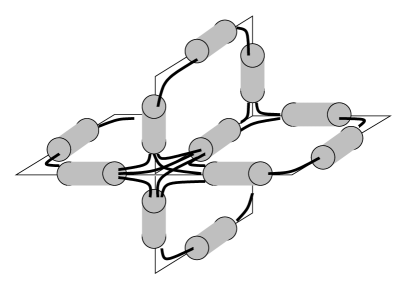
Figure 10: Piece of embedded circuit diagram for quantum BF theory. The picture shows a three dimensional example. Labels and arrows on wires are omitted.

Explicitly expanding the delta functions in the partition functions in characters we obtain

$$\mathcal{Z}_{\text{BF}}=\sum_{V_{f}}(\prod_{f}\dim_{V_{f}})\int\prod_{e}\mathrm{d}g_{e}\prod_{f}\chi_{V_{f}}(g_{1}\cdots g_{k}).$$ (3)

Here the sum runs over all assignments $V_{f}$ of irreducible representations to faces $f$. This corresponds diagrammatically to the expansion in Figure 2. One might consider this a more proper version of discrete BF theory than (2) as it contains explicit representation valued degrees of freedom which can be considered the discrete version of the $B$-field.

Reformulated in the spin foam formalism the partition function (3) yields in dimension three the Ponzano-Regge model [12] and in dimension four the Ooguri model [13].

5.1.2 Exact renormalization

The proof of topological invariance of (anomaly corrected) quantum BF theory in dimension three using the present formalism of circuit diagrams and certain cellular moves was already exhibited in [5]. We extend this here to a full renormalization treatment and perform the (surprisingly simple) generalization to arbitrary dimensions.

The first step in understanding the renormalization of quantum BF theory is to investigate the change of the partition function $\mathcal{Z}_{\text{BF}}$ under change of cellular decomposition. Thanks to Conjecture 2.4 it is sufficient to regard the change of $\mathcal{Z}_{\text{BF}}$ under the cellular moves.

move	initial configuration	final configuration
$n$
$n-1$
$n-2$

Table 1: The effect of the cellular moves on the circuit diagrams. The relevant cells as well as the embedded cables (boxes/cylinders) and wires (thicker lines) are shown.

As $\mathcal{Z}_{\text{BF}}$ is encoded in the embedded circuit diagram constructed above we need to compare the circuit diagrams before and after the application of the respective move. This is shown in Table 1. Only the parts of the circuit diagrams affected by the moves are shown. Furthermore, only the moves of type $n$, $n-1$ and $n-2$ are indicated. The other moves do not affect cells of dimension $\geq n-2$ and thus leave the circuit diagram unchanged.

So, how does the value of $\mathcal{Z}_{\text{BF}}$ change? Comparing Table 1 with Figures 4 and 6 we find that both the $n$ as well as the $n-1$ move leave $\mathcal{Z}_{\text{BF}}$ invariant. This is due respectively to the gauge fixing and the delta identity. By contrast, the $n-2$ move removes a factor corresponding to a closed $\Omega$-loop, i.e. a factor of $\kappa$.

Now we shall consider the renormalization of $\mathcal{Z}_{\text{BF}}$, i.e. we wish to construct an action of the cellular groupoid on parameters of the model such that $\mathcal{Z}_{\text{BF}}$ becomes invariant. The model as defined by (2) has no parameters. We need to modify it by introducing parameters. However, as we have seen we only have to compensate for factors of $\kappa$ which carry no local information of the model. It is sufficient to introduce a global integer parameter $p$ which counts these factors. We define the partition function of the modified model simply as

$$\tilde{\mathcal{Z}}_{\text{BF}}:=\kappa^{p}\mathcal{Z}_{\text{BF}}.$$ (4)

It remains to define the actions of the moves. We let the moves of type $n$, $n-1$, $n-3$, $n-4$, …act trivially while we let the move of type $n-2$ act by sending $p\mapsto p+1$ and its inverse by sending $p\mapsto p-1$. This precisely cancels the factor $\kappa$ appearing in the circuit diagram for the $n-2$-move. We obtain an exact renormalization.

The renormalized model has a free global parameter $p$. To specify it, one has to specify its value in a given cellular decomposition. This determines it, by the action of the renormalization groupoid, for all cellular decompositions. From the point of view of the classical continuum model the discretization allows an exact quantization (i.e. not depending on it) up to the anomaly manifest in $p$.

Alternatively, we can fix the extra parameter $p$ by making it explicitly depend on the numbers $c_{k}$ of cells of given dimension $k$ (as done to obtain topological invariants [2, 3, 4]). For example we can set

$$p:=-c_{n}+c_{n-1}-c_{n-2}.$$

It is easy to see that $p$ defined in this way is changed only by moves of type $n-2$, and exactly in the right way. Indeed we can make this part of the definition of the model instead of its renormalization. The action of the renormalization groupoid is then trivial. The model is then independent of the cellular decomposition, it is a renormalization groupoid fixed point. When referring to quantum BF theory in the following we will usually mean this version (4) where the anomaly has been fixed in some suitable way.

5.2 Generalized Yang-Mills theory

To talk about renormalization might seem somewhat artificial in the context of quantum BF theory. Indeed we saw that there is only one global parameter involved which can be easily absorbed into a redefinition of the partition function. As a less trivial example we discuss Yang Mills theory in this section.

It might seem surprising that we apparently wish to consider a theory that is defined on a metric background. However, we really consider a generalization of Yang-Mills theory that naturally arises in a discretized setting [1]. This provides a nice example of how a background structure can be turned into local parameters. These local parameters are then precisely what the renormalization groupoid acts on.

5.2.1 Discretization and quantization

We start again from a continuum formulation. Let $M$ be a compact manifold of dimension $n$, $G$ a compact Lie group and $P$ a principal $G$-bundle over $M$. Imagine we have some theory, determined through an action $S$ which depends on a connection $A$ on $P$. In order to define a quantum theory via a path integral

$$\mathcal{Z}=\int\mathcal{D}A\,e^{-S},$$

we discretize the manifold $M$ via a cellular decomposition $\mathcal{C}$ of $M$.

We proceed as above, i.e. we discretize the connection by associating parallel transports to edges $e$ and holonomies to faces $f$ of the 2-skeleton of the dual complex. The most general local gauge invariant action is then given by

$$S=\sum_{f}\sigma_{f}(g_{1}\cdots g_{k}),$$

where $g_{1},\dots,g_{k}$ are the group elements associated to the edges that bound the face $f$. $\sigma_{f}$ is a choice of class function for each face $f$. This yields the partition function

$$\mathcal{Z}_{\text{CGT}}=\int\prod_{e}\mathrm{d}g_{e}\prod_{f}\rho_{f}(g_{1}\cdots g_{k}),$$

where we set $\rho_{f}:=e^{-\sigma_{f}}$.

Indeed we see immediately that it is a generalization of the quantum BF theory partition function (2). Decomposing $\rho_{f}$ into characters

$$e^{-\sigma_{f}}=\sum_{V}\alpha_{V,f}\chi_{V},$$

yields

$$\mathcal{Z}_{\text{CGT}}=\sum_{V_{f}}(\prod_{f}\alpha_{V_{f},f})\int\prod_{e}\mathrm{d}g_{e}\prod_{f}\chi_{V_{f}}(g_{1}\cdots g_{k}).$$ (5)

Here the sum over irreducible representations for each face is taken to the front as a sum over assignments of an irreducible representation $V_{f}$ to each face $f$ (compare (3)). As (5) is a generalization of lattice gauge theory to cellular decompositions we call it cellular gauge theory in the following.

From this expression we can read off the diagrammatic representation of $\mathcal{Z}_{\text{CGT}}$ [1]. The circuit diagram is exactly the same embedded graph as for BF theory (Figure 10). Only now the summation over irreducible representations for each closed wire (corresponding to each face) cannot be hidden in $\Omega$ labels for the wires. Instead the wires must carry explicit labels and the sum over diagrams is performed with the weight factor $(\prod_{f}\alpha_{V_{f},f})$.

Note that the partition function (5) has locally infinitely many parameters. For each face $f$ there is a choice of parameter $\alpha_{V,f}$ for each irreducible representation $V$ (of which there are infinitely many). In the following we restrict ourselves to a more manageable situation. We set

$$\alpha_{V,f}:=(\dim V)\,e^{-\lambda_{f}C_{V}},$$ (6)

where $C_{V}$ is the value of the quadratic Casimir operator on $V$ and $\lambda_{f}$ is a positive real parameter depending on the face.

We now turn to the relation with Yang-Mills theory. Assume that $M$ is equipped with a flat metric and that $\mathcal{C}$ is a cellular decomposition of $M$ into hypercubes of equal side length $a$. We set all $\lambda_{f}$ equal to $\lambda:=a^{n-4}\gamma^{2}$. Then it can be shown that in the limit $a\to 0$ the action defined in this way approximates the continuum action of Yang-Mills theory (up to a constant)

$$S_{\text{YM}}=-\frac{1}{\gamma^{2}}\int_{M}\operatorname{tr}(F\wedge\star F),$$

with coupling constant $\gamma$. Indeed, this is at the foundation of lattice gauge theory (see e.g. [14]) and the discrete action we arrived at is nothing but the heat kernel action of lattice gauge theory. Note that that $\lambda$ plays the role of (the square of) a coupling constant.

$${\lx@xy@svg{\hbox{\raise 0.0pt\hbox{\kern 0.0pt\hbox{\ignorespaces\ignorespaces{\hbox{\lx@xy@droprule}}}}}}}\quad\xleftarrow[\lambda\to 0]{}\quad{\lx@xy@svg{\hbox{\raise 0.0pt\hbox{\kern 8.53578pt\hbox{\ignorespaces\ignorespaces{\hbox{\lx@xy@droprule}}\ignorespaces\ignorespaces{\hbox{\lx@xy@droprule}}{\hbox{\kern-8.53578pt\raise 0.0pt\hbox{\hbox{\kern 0.0pt\raise 0.0pt\hbox{\cirbuild@}}}}}{\hbox{\kern-2.91667pt\raise 0.0pt\hbox{\hbox{\kern 0.0pt\raise-3.47223pt\hbox{$\textstyle{\lambda}$}}}}}}}}}}\quad\xrightarrow[\lambda\to\infty]{}\quad{\lx@xy@svg{\hbox{\raise 0.0pt\hbox{\kern 8.53578pt\hbox{\ignorespaces\ignorespaces{\hbox{\lx@xy@droprule}}\ignorespaces\ignorespaces{\hbox{\lx@xy@droprule}}\ignorespaces\ignorespaces{\hbox{\lx@xy@droprule}}\ignorespaces\ignorespaces{\hbox{\lx@xy@droprule}}\ignorespaces\ignorespaces{\hbox{\lx@xy@droprule}}\ignorespaces\ignorespaces{\hbox{\lx@xy@droprule}}}}}}} \textstyle{\lambda} \textstyle{\lambda}$$

Figure 11: The two limits of the heat kernel operator.

Observe that the heat kernel operator $e^{-\lambda C}$ has two interesting limits, $\lambda\to 0$ and $\lambda\to\infty$. In the first case it just becomes the identity. In view of the above this implies that quantum BF theory can be considered the weak coupling limit ($\lambda=0$) of lattice gauge theory, since we then recover (3) from (5). The opposite regime ($\lambda\to\infty$) is that of strong coupling of lattice gauge theory. The low dimensional representations dominate more and more in the partition function. At the extreme point $\lambda=\infty$, only the trivial representation contributes, onto which the heat kernel operator becomes a projector. Diagrammatically the limits can be expressed as in Figure 11.

Let us go back to the case of interest, that of a topological manifold $M$ with arbitrary cellular decomposition $\mathcal{C}$. Note that the above relation also suggests to view $\lambda_{f}$ as a remnant of a local metric. As we shall see below this statement can be made precise in the case of dimension two.

Diagrammatically, the choice (6) means that we can put the heat kernel factor per face $f$ into the circuit diagram as a disc with label $\lambda_{f}$. The summation over irreducible representations with the remaining factor of dimension can then be indicated by $\Omega$-labels for all the wires.

5.2.2 Renormalization in general

We start by investigating the change in $\mathcal{Z}_{\text{CGT}}$ under the moves. Using the diagrammatic representation this step is almost identical to what we did for quantum BF theory. Indeed, again the relevant parts of the diagrams are as shown in Table 1. The difference is that we now sum over irreducible representations for each wire with a weight that is not the dimension, as can be indicated by an extra disc diagram per wire.

This makes no difference for the $n$-move, as the gauge fixing identity (Figure 4) does not depend on attached labels. For the $n-1$-move, however, the delta identity (Figure 6) that ensured invariance in the BF case can no longer be applied. The weight in the summation over representations for the closed wire is no longer the dimension. For the $n-2$-move there is again just a mismatch of a factor, which is now

$$\kappa_{f}:=\sum_{V}(\dim V)\alpha_{V_{f},f}=\sum_{V}(\dim V)^{2}e^{-\lambda_{f}C_{V}}.$$

In summary, the most crucial difference to quantum BF theory is the breaking of invariance under the $n-1$-move.

Let us turn to the problem of renormalization. As before, the treatment of the $n-2$-move is relatively easy. Redefining the partition function to be

$$\tilde{\mathcal{Z}}_{\text{CGT}}:=(\prod_{f}\kappa_{f}^{-1})\mathcal{Z}_{\text{CGT}},$$

fixes the $n-2$-move, i.e. makes $\tilde{\mathcal{Z}}_{\text{CGT}}$ invariant under it. On the other hand, this makes the non-invariance under the $n-1$-move worse in the sense that it would now be broken even in the limit $\lambda_{f}=0$. To remedy this and obtain the renormalization groupoid fixed point of quantum BF theory in this limit one could include a factor of $\kappa^{-c_{n}+c_{n-1}}$ (compare Section 5.1.2).

The renormalization of the $n-1$-move poses much deeper problems. Superficially it seems that instead of applying the delta identity, we have to apply the modified delta identity (Figure 8). Indeed we can do this and perhaps this is really a first step towards tackling the general problem. However, the circuit diagram we arrive at is not of the same kind as the original circuit diagram: The shifted heat kernel diagram extends over several wires.

Although no general solution to the problem is known, qualitative features of the renormalization groupoid flow are easily described. Firstly, the parameter space of cellular gauge theory contains two fixed points (we assume the anomaly has been fixed as described above). The first one, at $\lambda=0$ (weak coupling limit) is quantum BF theory while the second one at $\lambda=\infty$ (strong coupling limit) is a trivial theory. (In the latter all representations are trivial and invariance under the moves is trivially satisfied.)

Secondly, we can say something about the direction of the renormalization groupoid flow. Consider a region of the manifold with some given parameter values $\lambda_{f}$. Roughly speaking, we can perform a refinement without changing the partition function by assigning to the newly created parameters the topological value $\lambda_{f}=0$. Now the partition function in the refined region should be left unchanged if we average the parameters $\lambda_{f}$ in this region in some suitable way. That is, the average value of the parameters (of which there are now more) has decreased compared to the unrefined situation. In summary, if we coarsen, the parameters $\lambda_{f}$ must generally increase to keep the partition function fixed. The renormalization groupoid flow goes in the direction from lower values of $\lambda_{f}$ in the ultraviolet to higher values in the infrared.

This general behaviour applies in particular close to the renormalization groupoid fixed points. (Consider for example a situation where only a few $\lambda_{f}$ are non-zero or non-infinite.) Thus, quantum BF theory is a (repulsive) UV fixed point while the trivial theory is an (attractive) IR fixed point. This is schematically illustrated in Figure 12.

Figure 12: Qualitative picture of the renormalization groupoid flow for cellular gauge theory (generalized discrete quantum Yang-Mills theory). The two fixed-points are quantum BF theory in the weak coupling limit ($\lambda=0$) and the trivial theory in the strong coupling limit ($\lambda=\infty$). The general direction of the flow is from the first (UV) fixed-point to the second (IR).

5.3 Exact renormalization in dimension two

In the case of dimension two an exact renormalization can be performed which confirms the qualitative picture. As lattice gauge theory is solvable then [15] this is not at all surprising. That things can be made well in this case is rather obvious in our approach. As each cable has only two wires (because each edge bounds only two faces), the shifted heat kernel factor again sits on a single wire.

As there is no $n-2$-move in dimension $n=2$ we consider the original partition function $\mathcal{Z}_{\text{CGT}}$ (and not $\tilde{\mathcal{Z}}_{\text{CGT}}$). Now, after applying the modified delta identity, we can combine the shifted heat kernel factor with the one that was attached to the wire before via addition (Figure 4.2.a). We simply get the heat kernel factor for the sum of the parameters.

The solution of the renormalization problem in dimension two is thus as follows. The 2-move acts trivially. The 1-move acts by sending the pair of parameters $(\lambda_{f_{1}},\lambda_{f_{2}})$ to $\lambda^{\prime}_{f_{2}}=\lambda_{f_{1}}+\lambda_{f_{2}}$. Here, $f_{1}$ denotes the 0-cell (or face) that is removed, $f_{2}$ denotes the other 0-cell (or face) with which $f_{1}$ was connected through a 1-cell (edge). The new parameter value $\lambda^{\prime}_{f_{2}}$ replaces the old one for $f_{2}$. The so defined action leaves $\mathcal{Z}_{\text{CGT}}$ invariant and is local in the sense of Definition 3.2.

Note that the action is not defined for the whole cellular groupoid, but only in the direction of coarsening. (An action of the inverse 1-move is not defined.) This is due to the impossibility of unambiguously recreating local parameters and goes hand in hand with the idea of integrating out degrees of freedom (see the discussion at the end of Section 3.2).

Coming back to the interpretation of cellular gauge theory as Yang-Mills theory we can give the local parameters indeed a simple meaning in terms of metric information. We can think of $\lambda_{f}$ as (proportional to) the area of the face $f$. The 1-move might then be thought of as the merging of two faces, thus giving the new face the sum of the areas.

It is sometimes said that 2-dimensional Yang-Mills theory is topological. This is not true in our terminology, i.e. it is not a renormalization groupoid fixed point. However, its renormalization is exact and rather simple. Of course, it is even simpler in the context of lattice gauge theory where all local parameters are identical and thus only one parameter changes under change of scale.

As a side remark, we observe that it is very easy to solve the two dimensional theory using the diagrammatics [1]. Just apply the tensor product identity (Figure 5) to all cables. Only closed loops of wire without any cables are left. Counting the loops and taking care of the heat kernel factors one obtains immediately

$$\mathcal{Z}_{\text{CGT}}=\sum_{V}\,(\dim V)^{\chi}\,e^{-C_{V}\sum_{f}\lambda_{f}},$$

where $\chi=c_{2}-c_{1}+c_{0}$ is the Euler characteristic of $M$ and the sum runs as usual over the irreducible representations of $G$. This agrees of course with the well known solution of lattice gauge theory [15]. Moreover, the diagrammatic solution carries over directly to the quantum group case, yielding the same expression [1]. (Then “$\dim$” denotes the quantum dimension and $C_{V}$ some suitable quantum Casimir operator.)

6 Spin foam models of quantum gravity

In this section we consider certain spin foam models of Euclidean quantum gravity in the light of our approach to renormalization. These are the Reisenberger model [7], the Barrett-Crane model [8], and a new model interpolating between the latter and quantum BF theory.

For all considered models the problem of renormalization is nontrivial as they depend on the discretization of space-time in a nontrivial way. Finding a solution to the renormalization problem being far beyond the scope of this paper we limit ourselves to a first step. That is, we investigate the question of amenability of these models to a renormalization treatment. This implies identifying suitable local degrees of freedom that can be acted upon by the renormalization groupoid. Since these degrees of freedom are present neither in the Reisenberger model nor in the Barrett-Crane model we propose modifications of both models that carry such degrees of freedom.

6.1 Motivation: BF theory plus constraint

For the reader’s convenience we review very briefly the motivation of the present models as quantizations of general relativity (see [11] for more details).

Let $M$ be a compact four dimensional manifold (space-time) with a $\mathrm{Spin}(4)$ principal bundle. Consider a 1-form $e$ (the vierbein) with values in the Lie algebra of $\mathrm{Spin}(4)$ and a spin connection $A$. Let $F$ be the curvature 2-form of $A$ and consider the action

$$S=\int_{M}\operatorname{tr}(e\wedge e\wedge F).$$

This describes Euclidean general relativity (assuming $e$ to be non-degenerate).

While this is difficult to quantize one can observe a certain similarity with BF theory (1). Indeed we can take the BF action if we introduce the additional constraint that the $B$-field arises from an $e$-field, i.e.

$$B=e\wedge e.$$ (7)

The idea is now to quantize BF theory, which we know how to do (see Section 5.1) and impose the constraint (7) afterwards. The latter step is rather nontrivial and various proposals for its implementation have been made. Perhaps the best known ones are the model due to Reisenberger and the one due to Barrett and Crane. These are the ones we are going to discuss.

6.2 The Reisenberger model

Since the spin group in four dimensions is $\mathrm{Spin}(4)=\mathrm{SU}(2)\times\mathrm{SU}(2)$ we can decompose the spin bundle into two “chiral” components, one for each copy of $\mathrm{SU}(2)$. One can then observe that one chiral component is enough to formulate classical general relativity. This carries over to the above context of obtaining general relativity by constraining BF theory.

The Reisenberger model [7] thus starts with quantum BF theory (2) with gauge group $\mathrm{SU}(2)$. It is formulated on a simplicial decomposition of space-time. The partition function is given by

$$\mathcal{Z}_{\text{Rei}}=\int\prod_{e}\mathrm{d}g_{e}\prod_{v}(z\sqrt{2\pi})^{-5}[e^{-\frac{1}{2z^{2}}\Omega_{ij}\Omega^{ij}}]\prod_{f}\delta(g_{1}\cdots g_{k}).$$ (8)

What is different as compared to quantum BF theory is the factor

$$(z\sqrt{2\pi})^{-5}[e^{-\frac{1}{2z^{2}}\Omega_{ij}\Omega^{ij}}]$$ (9)

inserted for each vertex. $z$ is a real parameter of the model while $\Omega_{ij}$ denotes a certain operator. $\Omega_{ij}$ is a sum of operators each of which acts on a pair of delta functions associated with the given vertex. Diagrammatically speaking it acts on all pairs of wires (belonging to pairs of faces or 2-simplices) which are associated with the vertex (i.e. which belong to the 4-simplex). We will not give the full definition here as this is irrelevant for our considerations.

The model as defined is not immediately amenable to a treatment in our approach. A serious problem is the fact that it is only defined for simplicial decompositions. Thus, although the cellular moves can be applied in principle the resulting configurations are not simplicial and thus not comparable to the original model. An interesting alternative would be to try to define the model for cellular decompositions through the moves. However this would presumably involve solving the renormalization problem and is thus beyond the scope of our current investigation.

Another prerequisite to a renormalization in our sense are tunable local parameters. These are easily introduced into the partition function. One can simply let the real parameter $z$ depend on the vertex, i.e. introduce one $z_{v}$ per vertex. What is more, for $z_{v}\to\infty$ we (essentially, i.e. up to normalization) recover quantum BF theory. That is, our parameter space contains a renormalization groupoid fixed point (up to an anomaly which can be easily eliminated, see Section 5.1).

Figure 13: Qualitative picture of the renormalization groupoid flow for both the Reisenberger and the interpolating model. There is one ultraviolet fixed-point at $\lambda=0$ which is quantum BF theory. There is another special point at $\lambda=\infty$ (or $z=0$) which for the interpolating model corresponds to the Barrett-Crane model.

Assuming the difficulties can be overcome we can nevertheless make some qualitative remark on the the renormalization groupoid flow. For better comparability with the other models we consider inverted parameters $\lambda\cong z^{-1}$. We also disregard the first factor in (9) which should not be relevant for the qualitative picture. The model is rather similar to cellular gauge theory in the vicinity of the quantum BF theory fixed point. Indeed, in this region the arguments concerning the flow put forward in Section 5.2.2 apply. That is, the flow points away from the “weak coupling limit” $\lambda=0$ which is a repulsive ultraviolet fixed-point. On the other hand, the point $\lambda=\infty$ is not a fixed point and it is not clear how the flow behaves near it. Figure 13 shows a diagrammatic illustration of the situation.

6.3 The Barrett-Crane model

While different versions of the Euclidean Barrett-Crane model have been proposed [16, 17, 18, 19, 20] we consider a version which appears to be the most natural one in our framework. For ease of terminology we refer to it in the following as “the” Barrett-Crane model.

While originally defined for simplicial complexes only it was shown by Reisenberger that the Barrett-Crane model naturally extends to more general complexes [9]. Our treatment in the following directly applies to general cellular decompositions. It is closely related to the connection formulation of which an extensive treatment can be found in [19].

We start with the full $\mathrm{Spin}(4)$ BF theory in four dimensions. To describe the crucial step of implementing the constraint (7) it will be convenient to explicitly perform the decomposition into chiral components. Writing each group element and matrix element as a product of left-handed and right-handed chiral $\mathrm{SU}(2)$ component the partition function (2) decomposes into the product of two BF partition functions

$$\mathcal{Z}_{\text{BF}}=\int\prod_{e}\mathrm{d}g^{L}_{e}\mathrm{d}g^{R}_{e}\prod_{f}\delta(g^{L}_{1}\cdots g^{L}_{k})\delta(g^{R}_{1}\cdots g^{R}_{k}).$$ (10)

Here the superscripts $L$ and $R$ denote the chiral components.

This step finds its diagrammatic expression in the splitting of the circuit diagram for the partition function (Figure 10) into two identical diagrams for $\mathrm{SU}(2)$, one for each chiral component. Note that the representation labels for the diagrams are now $\mathrm{SU}(2)$ representation labels, summed over independently.

We stick in the following to a purely diagrammatic representation of the partition function. This avoids on the one hand writing complicated formulas and on the other hand facilitates understanding the structure of the model in view of the renormalization problem. It also avoids extra complications arising for non-simplicial decompositions in the spin foam formulation.

As a second step we replace each cable by a sequence of two cables. This is a special case of the (inverse) gauge fixing identity (Figure 4) and thus does not change the partition function. It implies algebraically another (redundant) doubling of the group variables, so that for each chiral component there is now one group variable attached to each end of each edge.

So far we have only rewritten the partition function without changing it. The Barrett-Crane model is now obtained by inserting further cables on each edge between the cables present. This is depicted in Figure 14. One cable is inserted for each chiral pair of wires, so that the pair of wires goes through the cable. This has the effect of projecting onto “simple” irreducible representations of $\mathrm{Spin}(4)$, i.e. those where both chiral components are the same representation of $\mathrm{SU}(2)$. It is designed to implement the constraint (7). The partition function $\mathcal{Z}_{\text{BC}}$ of the Barrett-Crane model is defined by this circuit diagram. The conversion of the diagram into a closed formula is again straightforward, by inserting a group integral for each cable etc.

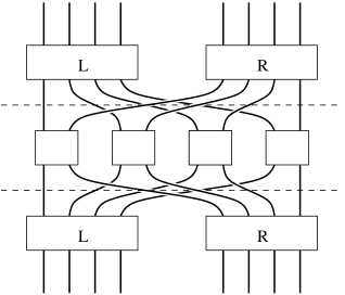
Figure 14: In going from BF theory to the Barrett-Crane model one inserts the cables between the dotted lines. There is one such cable for each chiral pair of wires. Here is shown an edge with four wires, the only case occurring in a simplicial decomposition in dimension four. Labels and arrows on wires are omitted.

Although the circuit diagram appears to be quite complicated at this point it can be simplified considerably. As the Barrett-Crane cables just carry two wires with irreducible representations we can apply the tensor product identity (Figure 5). This forces the two chiral components to lie in the same representation and and leads to a decomposition of the circuit diagram. Indeed we obtain a separate circuit diagram for each vertex (or $n$-cell). After repeated application of the gauge fixing identity (Figure 4) this consists of one cable per edge ($n-1$-cell) and one wire per face ($n-2$-cell) that meet the vertex ($n$-cell). An easy way to construct this diagram is as follows: Consider the part of the circuit diagram for BF theory that lies in an $n$-cell. Cut it out (this cuts cables in halves) and produce a mirror image. Now connect the diagram and its mirror image in the obvious way to obtain a closed diagram. The two parts correspond exactly to what were before the two chiral components. For a 4-cell which is a simplex the diagram obtained in this way is drawn in Figure 15.

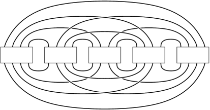
Figure 15: The circuit diagram for a 4-simplex in the Barrett-Crane model. Labels and arrows on wires are omitted.

The whole partition function can be reexpressed as

$$\mathcal{Z}_{\text{BC}}=\sum_{V_{f}}(\prod_{f}(\dim V_{f})^{2-|\partial f|})\prod_{v}A_{v}(V_{f}).$$ (11)

Here the summation is over labelings $V_{f}$ of faces with irreducible representations of $\mathrm{SU}(2)$, $|\partial f|$ denotes the number of edges of face $f$ and $A_{v}(V_{f})$ is the value of the circuit diagram for the vertex $v$ (with the appropriate labels). The origin of the exponent $|\partial f|$ lies in the fact that each application of the tensor product identity (Figure 5) produces a factor of inverse dimension.

Other versions of the Barrett-Crane model agree with the present one in the vertex amplitude $A_{v}(V_{f})$, while differing in the choice of weights for edges and faces. For example, the Perez-Rovelli version [17] is obtained if instead of inserting one layer of Barrett-Crane cables as in Figure 14 two such layers are inserted with another “LR layer” inbetween. We explain below why the present choice stands out in view of a renormalization treatment.

As a first step in investigating renormalization properties of the Barrett-Crane model we apply the moves to the model “as is”. One quickly sees that neither the $n$- nor the $n-1$-move preserve the partition function in any obvious way. Indeed, for the $n$-move one removes a subdivision between $n$-cells (i.e. merges two vertices) so that before the move one has two disconnected diagrams while afterwards there is one connected diagram. Except for trivial cases there seems to be no way how they could be equal. This is not a surprise. The relevant identity for quantum BF theory was the gauge fixing identity. It reflects the possibility of fixing a gauge and is based on gauge invariance (see [1]). However, the $\mathrm{Spin}(4)$ gauge invariance is precisely broken in the Barrett-Crane model (to a $\mathrm{SU}(2)$ subgroup) by the introduction of the extra cables which act as projectors.

For the $n-2$-move the situation is similar to quantum BF theory. Before the move one has factors of dimension which are not present after the move. See footnote 8 however.

6.4 An interpolating model

As the Barrett-Crane model is not invariant under the cellular moves, i.e. not topological, a renormalization treatment in our sense would require local parameters. On top of that one would like to have a renormalization groupoid fixed point in the ultraviolet analogous to the weak coupling regime in cellular gauge theory (Section 5.2) and the large $z$ regime in the Reisenberger model (Section 6.2).

Based on these requirements we propose a new model as follows: The Barrett-Crane model is defined as a modification of quantum BF theory (which is topological). It is thus natural to tune the way this modification is performed. More precisely, as above, we start with BF theory of $\mathrm{Spin}(4)$, rewriting it in terms of the chiral decomposition and the extra doubling of the cables for each edge. Then, instead of proceeding to insert cables as in Figure 14 we insert heat kernel factors as appearing in lattice gauge theory (see Section 5.2). Instead of arriving at the diagram of Figure 14 we arrive at the diagram of Figure 16 per edge. This defines the partition function $\mathcal{Z}_{\text{Int}}$ of the model.

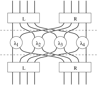
Figure 16: Edge diagrams for the interpolating model. $\lambda_{i}$ are positive real parameters. There is one such parameter per edge and face. Labels and arrows on wires are omitted.

The present definition uses the two limits of the heat kernel operator $e^{-\lambda C}$ (Figure 11). For $\lambda\to 0$ we recover quantum BF theory while for $\lambda\to\infty$ we get the usual Barrett-Crane model. The local parameters we have introduced are one positive real number per edge and face. If desired one could decrease the number of parameters by requiring them to be the same within a face or within an edge.

Considering qualitative aspects of the renormalization groupoid flow we have now the same scenario as for the Reisenberger model (Figure 13). At “weak coupling” (small $\lambda$) the arguments of Section 5.2.2 again apply. The renormalization groupoid flow is directed away from the ultraviolet fixed point given by quantum BF theory at $\lambda=0$. On the other hand, much less is known about the point $\lambda=\infty$ which corresponds to the Barrett-Crane model.

However, a numerical study of different versions of the Barrett-Crane model was conducted by Baez et al. [20]. This includes in particular the Perez-Rovelli version [17]. It turns out that the partition function in this case is strongly dominated by contributions with almost all representations trivial. It should be expected that our version of the Barrett-Crane model behaves somewhat similar, although not quite as extreme. This would suggest that at the point $\lambda=\infty$ of the interpolating model (where the Barrett-Crane model resides) we have “almost” a trivial theory, to be compared with the IR fixed point in cellular gauge theory.

In retrospect we have now an additional argument for our choice of weights for edges and faces for the Barrett-Crane model (manifest in (11)). We see now that it is not only natural in the way the model is constructed from quantum BF theory but essential in obtaining an ultraviolet fixed point in the parameter space of the interpolating model.

7 Discussion and conclusions

A crucial issue that we have not addressed in the present paper is the role of observables. Indeed, for a sensible physical interpretation what we need is not a renormalization that keeps the partition function fixed but one that preserves physical observables. Nevertheless, the two might be closely related. Indeed, for quantum BF theory the two notions coincide if we take observables to be Wilson loops. This is why (quantum group versions) of this model give rise both to invariants of manifolds and knots (the knots being Wilson loops), see [1]. The same is true for cellular gauge theory (quantum Yang-Mills theory) in dimension two. If we keep the “area” (the sum of the local parameters) inside a Wilson loop fixed, the expectation value of the latter is exactly preserved by the renormalization that we presented.

The situation is rather different for the models of quantum gravity that we have considered. Here, even the question of what the correct physical observables are is unresolved. Indeed, our qualitative statements concerning the renormalization groupoid flow could be (and probably will be) substantially altered if renormalization is performed with respect to relevant observables. A further point is that while we have considered these models for given topology and cellular decomposition it has been proposed to sum them over discretizations (usually simplicial ones) of space-time and even over topologies. However, to get control of such a sum it is presumably still necessary to understand and relate the individual terms (discretizations) and perform a renormalization in our sense.

One proposal for performing such a sum is that of a generating field theory [21, 13, 16, 22]. This is usually a field theory on the gauge group which generates discretized space-times as its Feynman diagrams. This is particularly easy to see when using our diagrammatic language. Expressing propagators and vertices in terms of the diagrams of Section 4, a closed Feynman diagram becomes exactly the circuit diagram representing the partition function of the respective model for the corresponding discretization.

In general, a renormalization with respect to observables is a weaker problem than a local renormalization with respect to the partition function. Namely, the latter implies the former but not the other way round. For example, in the quantum BF theory case, the anomaly cancels in expectation values. A related issue is that asking for an exact renormalization is often too much. A coarse discretization is not supposed to reproduce all the physics of a finer one. Thus, one usually requires a renormalization to preserve observables only in some approximate sense, for example have them converge in an “infinite refinement limit” as in lattice gauge theory.

While we have limited ourselves here to closed manifolds our framework extends straightforwardly to manifolds with boundary. Indeed, our definitions in Sections 2 and 3 carry over practically unchanged. In addition, gluing along boundaries is essentially straightforward for the models we consider. For quantum BF theory and cellular gauge theory this is already explained in [1]. In a setting with boundaries renormalization groupoid fixed points correspond to topological quantum field theories (at least if an exact renormalization of the partition function is required).

One could also envisage a special treatment of boundaries where they carry extra parameters. This might be desirable if a fixed background is attached to a boundary. Such a situation could occur for example if in quantum gravity one wishes to put quasi-classical or coherent states on the boundary.

As we have emphasized it is rather important for renormalization in our sense to work to allow for cellular decompositions and not restrict to simplicial ones. This is a problem in the Reisenberger model (considered in Section 6.2) whose definition strongly uses the fact that cells are simplices. A generalization of the model in this direction is thus desirable. In contrast, the formulation of the Barrett-Crane model (considered in Section 6.3) in terms of cellular decompositions is straightforward. In this case however, local parameters allowing for a renormalization groupoid flow are absent. This prompted us to define an interpolating model that contains both the Barrett-Crane model and quantum BF theory in its (local) parameter space. To define this we “imported” the idea of heat kernel factors from lattice gauge theory. This allows a continuous switching between a “weak coupling limit” of quantum BF theory and the “strong coupling limit” of the Barrett-Crane model.

We suggested that the renormalization groupoid flow both in the Reisenberger and in the interpolating model should behave similarly as for cellular gauge theory in the region of “weak coupling” (small $\lambda$). All these models share the same renormalization groupoid fixed point of quantum BF theory in the ultraviolet. On the other hand, while having a special point in the “strong coupling limit” of $\lambda=\infty$ this is an infrared fixed point only for cellular gauge theory. Nevertheless, both for the Reisenberger model and for the interpolating model one should expect behaviour somewhat similar to cellular gauge theory also in this region. In both cases, there are projection operators which are “maximally turned on” at $\lambda=\infty$ comparable to the heat kernel operators in cellular gauge theory. In contrast to the latter they do not lead to a complete restriction to trivial representations. Nevertheless, they should have an effect approaching this.

For the Barrett-Crane model numerical investigations by Baez et al. seem to indicate indeed that the partition function is strongly dominated by terms where almost all representations are trivial [20]. Baez et al. suggest that such a situation might indicate a bad choice of weights for edges and faces. Our conclusion is rather different. We propose that the Barrett-Crane model should be considered as just a point in the parameter space of a more general model (the interpolating model) which is rather more amenable to a renormalization. From this point of view it is even a welcome feature if the Barrett-Crane partition function is strongly dominated by terms with almost all representations trivial. This would give the interpolating model at “strong coupling” a region in parameter space which “almost” contains an infrared fixed point of the renormalization groupoid.

Markopoulou has made the interesting proposal [25, 26] to apply the renormalization methods of perturbative quantum field theory to spin foam models. Based on the structural similarity of spin foams with Feynman diagrams (which becomes a strict correspondence in the generating field theory approach mentioned above) she suggests a Bogoliubov type recursion equation for spin foams (formulated in a Hopf algebraic language). Her concept of coarsening is strictly based on spin foams but essentially coincides with the one coming from cellular decompositions in this context. Thus, one might hope that her approach can fruitfully complement the one presented here. In particular, Markopoulou’s approach might be useful in eliminating certain infinities (as the corresponding techniques in perturbative quantum field theory do). Such infinities arise for example from summing over infinitely many irreducible representations, as in quantum BF theory, compare (3).

The basic ideas on renormalization introduced in Sections 2 and 3 are not specific to the gauge type models that we have considered in the later sections. Indeed they should be applicable to a wide range of models (including spin systems for example). Furthermore, while we have emphasized the role of background independence, this is not a requirement. Indeed, the proposed methods might be applicable to situations where a metric background is present, but the discretization of space-time is nevertheless irregular (as in “random geometry” models). In such a situation metric information might be converted into local parameters. Indeed, we saw that this was a possible point of view in our cellular gauge theory example of Section 5.2.

Much of our treatment seems to depend on Conjecture 2.4 and indeed it would be important to establish its validity (or non-validity). However, the situation is rather less serious. Firstly, even if the conjecture was false in its present form, it is very likely to hold under some mild technical assumptions about the manifold or cellular decomposition (such as piecewise linearity). Such assumptions very likely would have little or no physical relevance. Secondly, for the application to a given model it is usually not necessary that the conjecture holds in all its aspects. For example, for all the models considered in this paper only the cells of dimension $n$, $n-1$, and $n-2$ are relevant. Thus, a much weaker form of the conjecture suffices. Thirdly, considering a certain subclass of refinements or coarsenings might be enough for a sensible renormalization in a given context. Again, this would require only a weaker form of the conjecture.

While we worked throughout with a topological manifold it should be possible to do away even with this “background”. A suitable setting in the present context would probably be that of (finite) CW-complexes. Conjecture 2.4 is definitely false if “$n$-dimensional manifold” is replaced by “$n$-dimensional CW-complex”. This is not surprising as the complex can contain “pieces” of lower dimension. On the other hand one could consider all cellular moves for all dimensions up to $n$ (the dimension of the cell of maximal dimension). This would give $n(n+1)/2$ moves. The analogue of Conjecture 2.4 would then state something like that any two finite decompositions as CW-complexes (if they exist) of the same topological space are related by a sequence of these moves. The basic considerations of Section 3 concerning renormalization could then be carried over practically unchanged. One could be even more general by considering combinatorial complexes. However, a quantum group generalization of models as considered here would be definitely lost in this case as it depends on certain topological information [1].

Acknowledgements

I would like to thank Hendryk Pfeiffer and Carlo Rovelli for valuable comments on the manuscript. Furthermore, I would like to thank Thomas Krajewski and Valentin Zagrebnov for discussions. This research was supported by the European Union through a Marie Curie Fellowship grant.

References

- [1] R. Oeckl, Generalized Lattice Gauge Theory, Spin Foams and State Sum Invariants, to appear in J. Geom. Phys., Preprint hep-th/0110259, 2001.
- [2] V. G. Turaev and O. Ya. Viro, State sum invariants of -manifolds and quantum -symbols, Topology 31 (1992), 865–902.
- [3] J. W. Barrett and B. W. Westbury, Invariants of piecewise-linear -manifolds, Trans. Amer. Math. Soc. 348 (1996), 3997–4022.
- [4] L. Crane, L. H. Kauffman, and D. N. Yetter, State-Sum Invariants of 4-Manifolds, J. Knot Theory Ram. 6 (1997), 177–234.
- [5] F. Girelli, R. Oeckl, and A. Perez, Spin foam diagrammatics and topological invariance, Class. Quantum Grav. 19 (2002), 1093–1108.
- [6] J. Ambjørn, B. Durhuus, and T. Jonsson, Quantum Geometry: A statistical field theory approach, Cambridge University Press, Cambridge, 1997.
- [7] M. P. Reisenberger, A simplicial spin foam model of 4-d Euclidean general relarivity, Preprint.
- [8] J. W. Barrett and L. Crane, Relativistic spin networks and quantum gravity, J. Math. Phys. 39 (1998), 3296–3302.
- [9] M. P. Reisenberger, On relativistic spin network vertices, J. Math. Phys. 40 (1999), 2046–2054.
- [10] U. Pachner, P.L. homeomorphic manifolds are equivalent by elementary shellings, European J. Combin. 12 (1991), 129–145.
- [11] J. C. Baez, An Introduction to Spin Foam Models of Theory and Quantum Gravity, Geometry and quantum physics (Schladming, 1999), Lecture Notes in Phys., no. 543, Springer, Berlin, 2000, pp. 25–93.
- [12] G. Ponzano and T. Regge, Semiclassical limit of Racah coefficients, Spectroscopic and Group Theoretical Methods in Physics (F. Bloch et al., ed.), North-Holland, Amsterdam, 1968.
- [13] H. Ooguri, Topological lattice models in four dimensions, Mod. Phys. Lett. A 7 (1992), 2799–2810.
- [14] M. Creutz, Quarks, gluons and lattices, Cambridge University Press, Cambridge, 1983.
- [15] A. A. Migdal, Recursion equations in gauge field theories, Sov. Phys. JETP 42 (1976), 413–418.
- [16] R. De Pietri, L. Freidel, K. Krasnov, and C. Rovelli, Barrett-Crane model from a Boulatov-Ooguri field theory over a homogeneous space, Nucl. Phys. B 574 (2000), 785–806.
- [17] A. Perez and C. Rovelli, A spin foam model without bubble divergences, Nucl. Phys. B 599 (2001), 255–282.
- [18] D. Oriti and R. Williams, Gluing 4-simplices: a derivation of the Barrett-Crane spin foam model for Euclidean quantum gravity, Phys. Rev. D 63 (2001), 024022.
- [19] H. Pfeiffer, Dual variables and a connection picture for the Euclidean Barrett-Crane model, Class. Quantum Grav. 19 (2002), 1109–1137.
- [20] J. C. Baez, J. D. Christensen, T. R. Halford, and D. C. Tsang, Spin foam models of Riemannian quantum gravity, Class. Quant. Grav. 19 (2002), 4627–4648.
- [21] D. V. Boulatov, A model of three-dimensional lattice gravity, Mod. Phys. Lett. A 7 (1992), 1629–1646.
- [22] M. Reisenberger and C. Rovelli, Spacetime as a Feynman diagram: the connection formulation, Class. Quant. Gravity 18 (2001), 121–140.
- [23] R. Oeckl, Braided Quantum Field Theory, Commun. Math. Phys. 217 (2001), 451–473.
- [24] R. Oeckl, Introduction to Braided Quantum Field Theory, Int. J. Mod. Phys. B 14 (2000), 2461–2466.
- [25] F. Markopoulou, An algebraic approach to coarse graining, Preprint hep-th/0006199, 2000.
- [26] F. Markopoulou, Coarse graining in spin foam models, Preprint gr-gc/0203036, 2002.