A new class of obstructions to the smoothness of null infinity

Abstract

Expansions of the gravitational field arising from the development of asymptotically Euclidean, time symmetric, conformally flat initial data are calculated in a neighbourhood of spatial and null infinities up to order 6. To this ends a certain representation of spatial infinity as a cylinder is used. This set up is based on the properties of conformal geodesics. It is found that these expansions suggest that null infinity has to be non-smooth unless the Newman-Penrose constants of the spacetime, and some other higher order quantities of the spacetime vanish. As a consequence of these results it is conjectured that similar conditions occur if one were to take the expansions to even higher orders. Furthermore, the smoothness conditions obtained suggest that if a time symmetric initial data which is conformally flat in a neighbourhood of spatial infinity yields a smooth null infinity, then the initial data must in fact be Schwarzschildean around spatial infinity.

1 Introduction

Penrose introduced the seminal idea that the gravitational field of isolated systems can be conveniently described by means of the notion of asymptotic simplicity [22] . Central to the concept of asymptotic simplicity is the idea —expectation— that the conformal boundary of the spacetime —null infinity, ${I}$— should possess a smooth differentiable structure. This approach to the description of isolated bodies in General Relativity is usually known as Penrose’s proposal —see e.g. [18, 19]. Static and stationary spacetimes have been shown to be (weakly) asymptotically simple, with a smooth null infinity [7]. However, the main purpose behind introducing the concept of asymptotic simplicity is to provide a suitable framework for the discussion of radiation. In spite of its elegance and aesthetical appeal, Penrose’s proposal is of little use if one is not able to prove that there exists a big family of non-trivial (in the radiative sense) asymptotically simple solutions to the Einstein Field Equations. A programme aimed to investigate the existence of such solutions, and provide a conclusive “answer” to Penrose’s proposal has been started by Friedrich —see e.g. [11, 12, 13, 14, 15, 16, 17]. His strategy is based on the use of the so-called Conformal Field Equations, which allow us to work and prove existence statements directly in the conformally rescaled, “unphysical” spacetime. Along this lines, Friedrich has been able to prove a semiglobal existence result that ensures that hyperboloidal initial data close to Minkowski data yields an asymptotically simple development which includes the point $i^{+}$ (future timelike infinity) [15]. Recently, Chruściel & Delay [2] —retaking an old idea by Cutler & Wald [6]— using a refined version of some initial data set constructed by Corvino [5] have been able to prove the existence of a big class of non-trivial (radiative) asymptotically simple spacetimes. Corvino’s initial data is constructed so that it is Schwarzschildean in a neighbourhood of spatial infinity, $i^{0}$. This means that the radiation content in the spacetime arising from the development of the data is somehow special. This can be seen directly from the fact that the Newman-Penrose constants of the spacetime are zero [9, 27]. Chruściel & Delay’s result is no doubt very important. However, it is not as general as one would like.

It has been suspected for a long time now that the region of spacetime where null infinity and spatial infinity meet is somehow problematic —see e.g. [23]. From the analysis of the hyperboloidal initial value problem it turns out that the smoothness of null infinity is preserved by the evolution if smooth data sufficiently close to Minkowski data are prescribed. The latter indicates that somehow the “decision” of having a smooth structure at null infinity is made in an arbitrarily small neighbourhood of spatial infinity. In some sense, Corvino’s data avoids all the intricacies and complications of this region of spacetime by setting the asymptotic end in the simplest way which is consistent with the presence of a non-vanishing ADM mass on the initial hypersurface. In connection with this, Friedrich [17] has performed a detailed first analysis of the behaviour of the gravitational field arising from asymptotically Euclidean, time symmetric initial data in the region where null infinity “touches” spatial infinity. By means of a novel representation of spatial infinity in which the point $i^{0}$ of the standard conformal picture is blown up to a cylinder $I$ — the cylinder at spatial infinity— a certain regularity condition on the Cotton-Bach tensor and symmetrised higher order derivatives of it has been obtained. The hope was that this regularity condition would ensure the smoothness of null infinity, at least in the region close to $i^{0}$ and ${I}$. A subsequent analysis by Friedrich & Kánnár [20] of the first orders of some expansions that can be obtained by evaluating the Conformal Field Equations at $I$, lead to conjecture that Friedrich’s regularity condition is the only condition one has to impose on time symmetric, initial data possessing an analytic compactification in order to obtain a development with smooth null infinity [19]. More precisely,

Conjecture (Friedrich, 2002).

There exists an integer $k_{*}>0$ such hat for given $k\leq k_{*}$ the time evolution of an asymptotically Euclidean, time symmetric, conformally smooth initial data set admits a conformal extension to null infinity of class $C^{k}$ near spacelike infinity, if the Cotton-Bach spinor satisfies the condition,

$$D_{(a_{s}b_{s}}\cdots D_{a_{1}b_{1}}b_{abcd)}(i)=0,\quad s=0,1,\ldots$$

for a certain integer $s_{*}=s_{*}(k)$. If the extension is of class $C^{\infty}$ then the condition should hold to all orders.

The objective of this paper is to provide a further insight into the conjecture above. It will turn out that the conjecture, as it stands, is false. In order to see why this is the case, the expansions of Kánnár & Friedrich will be carried to an even higher order. This requires the implementation of the Conformal Field Equations on a computer algebra system (Maple V). It should be emphasized that despite the use of the computer to perform the expansions, the results here presented are exact up to the order carried out. In order to simplify our discussion, the analysis will be restricted to developments of time symmetric conformally flat initial data. The time symmetry requirement stems from the fact that Friedrich’s analysis has only yet been carried for this class of data. A similar analysis of initial data with non-vanishing second fundamental form lies still in the future. However, some first steps have already been carried out [8]. The conformal flatness of the data ensures that the initial data satisfies the regularity condition trivially. Again, the construction of non-conformally flat data satisfying Friedrich’s regularity condition is a non-trivial endeavour whose undertaking will be left for future studies. In the light of the results here presented, it turns out that the restriction to the class of conformally flat data is not a drawback. Furthermore, it is not hard to guess how the results could generalise in the case of general time symmetric data.

The principal result of our investigation is the following,

Theorem (Main theorem).

Necessary conditions for the development of initial data which are time symmetric, conformally flat in a neighbourhood $B_{a}(i)$ of (spatial) infinity to be smooth at the intersection of null infinity and spatial infinity are that the Newman-Penrose constants $G^{(5)}_{k}$, $k=0,\ldots,4$ and the higher order Newman-Penrose constants, $G^{(6)}_{k}$, $k=0,\ldots,6$ vanish.

A more precise formulation of the theorem, including the definition of the Newman-Penrose constants and the higher order Newman-Penrose constants in terms of the initial data will be given in the main text.

We note that the previous conditions are fulfilled by the Schwarzschild initial data. The theorem has been obtained from the analysis, up to order $p=6$ of expansions constructed from the solutions of the transport equations induced by the conformal field equations upon evaluation on the cylinder at spatial infinity. From the evidence provided by the equations it is not unreasonable to conjecture that similar conditions arise if one were to obtain expansions to even higher orders. In [17] it was shown that the whole set up of the cylinder at spatial infinity is completely regular for Schwarzschildean data. Thus, the hypothetic new conditions must be satisfied by the Schwarzschild initial data. It is on this ground that the following conjecture is put forward:

Conjecture (New conjecture).

If an initial data set which is time symmetric and conformally flat in a neighbourhood $B_{a}(i)$ of the point $i$ yields a development with a smooth null infinity, then the initial data are in fact Schwarzschildean in $B_{a}(i)$.

Again, a more technical version of the conjecture is given in the main text.

The article is structured as follows: in section 2 a brief summary of the description of spacetime in the neighbourhood of spatial and null infinities in terms of the cylinder at spatial infinity is given. This digest has the intention of providing all the tools needed for the calculations described in the present article. Particular attention is paid to the spatial 2-spinor formalism and to the expansions of functions on $S^{3}$ in terms of unitary representations of $SU(2,\mbox{\SYM C})$. The reader is, in any case, remitted to [17] for a more extensive discussion. In section 3, the conformal field equations written in the conformal geodesic gauge are discussed. The initial data for the latter in the case of an asymptotically Euclidean, time symmetric, conformally flat initial hypersurface are described. The transport equations implied by the conformal field equations on the cylinder at spatial infinity are introduced in section 4. In order to properly motivate the calculations carried out in later sections, a careful discussion of their properties is undertaken. Section 5 contains the new results to be presented in the article. Here a description of the solution of the transport equations is done. Due to the large size of the expressions involved, the description will be focused on what we believe are the most relevant features of the solutions. However, it should be emphasized that everything has been explicitly calculated. The main conclusions extracted from the calculations is presented as our main theorem. In order to understand the meaning of the conditions presented in the main theorem, the Schwarzschild solution is discussed in this context, and a conjecture is formulated. Finally, in section 6, some conclusions and extensions of the present work are considered. There is also an appendix in which the implementation of the transport equations and how to solve them in the computer algebra system Maple V is briefly considered.

2 Spacetime in a neighbourhood of spatial infinity

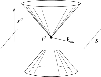
Let $(\widetilde{M},\widetilde{g}_{\mu\nu})$ be a vacuum spacetime arising as the development of asymptotically Euclidean, time symmetric, conformally analytic initial data $(\widetilde{S},\widetilde{h}_{\alpha,\beta})$. Later, we will restrict the class of initial data sets under discussion to those conformally flat around infinity. Assume for simplicity that $\widetilde{S}$ possesses only one asymptotic end. Let $i$ be the infinity corresponding to that end. The point $i$ is obtained by conformally compactifying the initial hypersurface $\widetilde{S}$, with an analytic conformal factor $\Omega$ which can be obtained from solving the time symmetric constraint equations. The compact 3 dimensional manifold obtained in this way will be denoted by $S$, and the conformally rescaled 3-metric by $h_{\alpha\beta}$. Assume that the 3-metric $h_{\alpha\beta}$ is analytic in an open ball $B_{a}(i)$ of radius $a$ centered on $i$. Let $\rho$ denote the geodesic distance along geodesics starting at $i$. The radius $a$ of the ball $B_{a}(i)$ is chosen such that $B_{a}(i)$ is geodesically convex.

Now, let $\widetilde{N}\cap\widetilde{M}$ be the domain of influence of the ball $B_{a}(i)\cap S$. Intuitively, one expects $N$ to cover a region of spacetime “close to null and spatial infinities”. In reference [17] it has been shown that once the time symmetric constraint equations have been solved, a certain gauge based on the properties of conformal geodesics can be introduced. Let $\tau$ be the parameter along these curves. This gauge has the property of producing a conformal factor $\Theta$ which can be in turn used to rescale the region $\widetilde{N}$ to obtain a “finite representation” $N$, of spacetime in a neighbourhood of spatial and null infinities. The relevant conformal factor is given by,

$$\Theta=\kappa^{-1}\Omega\left(1-\tau^{2}\frac{\kappa^{2}}{\omega^{2}}\right),$$ (1)

where $\omega$ is given by,

$$\omega=\frac{2\Omega}{\sqrt{|D_{a}\Omega D^{a}\Omega|}},$$ (2)

and $\kappa$ is a smooth function such that $\kappa=\kappa^{\prime}\rho$ with $\kappa^{\prime}(i)=1$. It contains the remaining piece of conformal freedom in our setting.

Throughout this work, space 2-spinors will be systematically used. In order to avoid problems with vanishing frame vectors on surfaces diffeomorphic to spheres, our discussion will be carried not on $N$ but on a subbundle $C_{a,\kappa}$ of the frame bundle over $N$. The subbundle $C_{a,\kappa}$ can be shown to be a 5-dimensional submanifold of $\mbox{\SYM R}\times\mbox{\SYM R}\times SU(2,\mbox{\SYM C})$ with structure group $U(1)$. More precisely, we define $C_{a,\kappa}$ to be given by,

$$C_{a,\kappa}=\left\{(\tau,\rho,t)\in\mbox{\SYM R}\times\mbox{\SYM R}\times SU(2,\mbox{\SYM C})|\;0\leq\rho<a,\;\;-\frac{\omega}{\kappa}\leq\tau\leq\frac{\omega}{\kappa}\right\}.$$ (3)

The projection $\pi^{\prime}$ of $C_{a,\kappa}$ into $N$ corresponds to the Hopf map $SU(2,\mbox{\SYM C})\rightarrow SU(2,\mbox{\SYM C})/U(1)\approx S^{2}$. Scalar fields and tensorial fields on $N$ are lifted to $C_{a,\kappa}$. Their “angular” dependence will be then given in terms of functions of $t\in SU(2,\mbox{\SYM C})$.

The manifold $C_{a,\kappa}$ has the following important submanifolds,

$$I=\{(\tau,\rho,t)\in C_{a,\kappa}\;|\;\rho=0,\;\;|\tau|<1\},$$ (4a)

$$I^{\pm}=\{(\tau,\rho,t)\in C_{a,\kappa}\;|\;\rho=0,\;\;\tau=\pm 1\},$$ (4b)

$${I}^{\pm}=\left\{(\tau,\rho,t)\in C_{a,\kappa}\;|\;\rho>0,\;\;\tau=\pm\frac{\omega}{\kappa}\right\}.$$ (4c)

2.1 Space 2-spinors

Consider the antisymmetric spinors $\epsilon_{ab}$, $\epsilon^{ab}$, $a,b=0,1$. These satisfy $\epsilon_{01}=1$, $\epsilon^{01}=1$. Let $\tau^{aa^{\prime}}$ denote the tangent vector to the conformal geodesics parametrised by $\tau$. We set,

$$\tau^{aa^{\prime}}=\epsilon_{0}^{\phantom{0}a}\overline{\epsilon}_{0^{\prime}}^{\phantom{0^{\prime}}a^{\prime}}+\epsilon_{1}^{\phantom{1}a}\overline{\epsilon}_{1^{\prime}}^{\phantom{1^{\prime}}a^{\prime}}.$$ (5)

In order to define introduce differential operators on $SU(2,\mbox{\SYM C})$ we consider the basis

$$u_{1}=\frac{1}{2}\left(\begin{array}[]{cc}0&i\\ i&0\\ \end{array}\right),\quad u_{2}=\frac{1}{2}\left(\begin{array}[]{cc}0&-1\\ 1&0\\ \end{array}\right),\quad u_{3}=\frac{1}{2}\left(\begin{array}[]{cc}i&0\\ 0&-i\\ \end{array}\right),$$ (6)

of the Lie algebra of SU(2,ℂ). Note that in particular, $u_{3}$ generates $U(1)$. Denote by $Z_{i}$, $i=1,2,3$ the real left invariant vector field generated by $u_{i}$ on SU(2,ℂ). We define the, following complex vector fields

$$X_{+}=-(Z_{2}+iZ_{1}),\quad X_{-}=-(Z_{2}-iZ_{1}),\quad X=-2iZ_{3}.$$ (7)

These are such that $[X_{+},X_{-}]=-X$. With the help of $X_{\pm}$ one can construct the following (frame) vectors fields,

$$c_{ab}=c^{0}_{aa^{\prime}}\partial_{\tau}+c^{1}_{aa^{\prime}}\partial_{\rho}+c^{+}_{aa^{\prime}}X_{+}+c^{-}_{aa^{\prime}}X_{-},$$ (8)

on $C_{a,\kappa}$. The use of a space spinor formalism based on the vector field $\sqrt{2}\partial_{\tau}=\tau^{aa^{\prime}}c_{aa^{\prime}}$ allows to perform our whole discussion in terms of quantities without primed indices. Accordingly, we write

$$c_{aa^{\prime}}=\frac{1}{\sqrt{2}}\tau_{aa^{\prime}}\partial_{\tau}-\tau^{b}_{\phantom{b}a^{\prime}}c_{ab}$$ (9)

with $c_{ab}=\tau_{(a}^{\phantom{(a}b^{\prime}}c_{b)b^{\prime}}=c^{0}_{ab}\partial_{\tau}+c^{1}_{ab}\partial_{\rho}+c^{+}_{ab}X_{+}+c^{-}_{ab}X_{-}$. The connection is represented by coefficients $\Gamma_{abcd}$ which can be decomposed in the form,

$$\Gamma_{abcd}=\frac{1}{\sqrt{2}}\left(\xi_{abcd}-\chi_{(ab)cd}\right)-\frac{1}{2}\epsilon_{ab}f{cd},$$ (10)

where the fields entering in the decomposition possess the following symmetries: $\chi_{abcd}=\chi_{ab(cd)}$, $\xi_{abcd}=\xi_{(ab)(cd)}$, $f_{ab}=f_{(ab)}$. The curvature will be described by the rescaled conformal Weyl spinor $\phi_{abcd}=\phi_{(abcd)}$, and by the spinor field $\Theta_{abcd}=\Theta_{ab(cd)}$ which encodes information relative to the Ricci part of the curvature. For the purpose of writing the field equations it will be customary to consider it decomposed in terms of $\Theta_{g\phantom{g}cd}^{\phantom{g}g}$ and $\Theta_{(ab)cd}$.

For latter use it is noted that an arbitrary four indices spinor $X_{abcd}$ can be written in terms of the “elementary spinors” $\epsilon^{i}_{abcd}$, $\epsilon_{ac}x_{bd}+\epsilon_{bd}x_{ac}$, $\epsilon_{ac}y_{bd}+\epsilon_{bd}y_{ac}$, $\epsilon_{ac}z_{bd}+\epsilon_{bd}z_{ac}$, and $h_{abcd}$ where,

$$x_{ab}=\sqrt{2}\epsilon_{(a}^{\phantom{a}0}\epsilon_{b)}^{\phantom{b)}1},\quad y_{ab}=-\frac{1}{\sqrt{2}}\epsilon_{a}^{\phantom{a}1}\epsilon_{b}^{\phantom{b}1},\quad z_{ab}=\frac{1}{\sqrt{2}}\epsilon_{a}^{\phantom{a}0}\epsilon_{b}^{\phantom{b}0},$$ (11)

and,

$$\epsilon^{i}_{abcd}=\epsilon_{(a}^{\phantom{(a}(e}\epsilon_{b}^{\phantom{b}f}\epsilon_{c}^{\phantom{c}g}\epsilon_{d)}^{\phantom{d)}h)_{i}},\quad h_{abcd}=-\epsilon_{a(c}\epsilon_{d)b}.$$ (12)

The notation $(abcd)_{i}$ means that the indices are to be symmetrised and then $i$ of them set to $1$. We write,

$$X_{abcd}=X_{0}\epsilon^{0}_{abcd}+X_{1}\epsilon^{1}_{abcd}+X_{2}\epsilon^{2}_{abcd}+X_{3}\epsilon^{3}_{abcd}+X_{4}\epsilon^{4}_{abcd}$$

$$\phantom{X_{abcd}=XX}+X_{x}(\epsilon_{ac}x_{bd}+\epsilon_{bd}x_{ac})+X_{y}(\epsilon_{ac}y_{bd}+\epsilon_{bd}y_{ac})+X_{z}(\epsilon_{ac}z_{bd}+\epsilon_{bd}z_{ac})$$

$$\phantom{X_{abcd}=XXXX}+X_{h}h_{abcd}.$$ (13)

2.2 Expansions of functions on $C_{a,\kappa}$

In order to obtain our expansions of the gravitational field around spatial infinity, we will require to decompose the functions arising into their diverse spherical (harmonic) sectors. Any function real analytic complex value function $f$ on $SU(2,\mbox{\SYM C})$ can be expanded in terms of some functions $\sqrt{m+1}\;T_{m\phantom{k}j}^{\phantom{m}k}$ forming a complete set in $L^{2}(\mu,SU(2,\mbox{\SYM C}))$ where $\mu$ is the standard Haar measure in $SU(2,\mbox{\SYM C})$. One has,

$$f(t)=\sum^{\infty}_{m=0}\sum^{m}_{j=0}\sum^{m}_{k=0}f_{m,k,j}T_{m\phantom{k}j}^{\phantom{m}k}.$$

The functions $T_{m\phantom{k}j}^{\phantom{m}k}$ can be shown to be related with the standard spin-weighted spherical harmonics. Using the fact that the group $SU(2,\mbox{\SYM C})$ is diffeomorphic to $S^{3}$, one can use the coordinates $(\zeta,\overline{\zeta},\alpha)$ to write a given $t\in SU(2,\mbox{\SYM C})$ as,

$$t\in\frac{1}{\sqrt{1+\zeta\overline{\zeta}}}\left(\begin{array}[]{cc}e^{i\alpha}&ie^{-i\alpha}\zeta\\ ie^{i\alpha}\overline{\zeta}&e^{i\alpha}\\ \end{array}\right).$$ (14)

The latter yields the following correspondence rule between the functions $T_{m\phantom{k}j}^{\phantom{m}k}$ and the spin-weighted spherical harmonics ${}_{s}Y_{ln}$:

$${}_{s}Y_{nm}\mapsto(-i)^{s+2n-m}\sqrt{\frac{2n+1}{4\pi}}T_{2n\phantom{n-m}n-s}^{\phantom{2n}n-m}.$$ (15)

The operators $X_{\pm}$ and $X$ (related to the NP $\eth$ and $\overline{\eth}$ operators) introduced in the previous sections can be seen to yield, upon application to the $T_{m\phantom{k}j}^{\phantom{m}k}$ functions the following,

$$X_{+}T_{m\phantom{k}j}^{\phantom{m}k}=\beta_{m,j}T_{m\phantom{k}j-1}^{\phantom{m}k},$$ (16a)

$$X_{-}T_{m\phantom{k}j}^{\phantom{m}k}=-\beta_{m,j+1}T_{m\phantom{k}j+1}^{\phantom{m}k},\qquad\mbox{with }\beta_{m,j}=\sqrt{j(m-j+1)}.$$ (16b)

A function $f$ on $SU(2,\mbox{\SYM C})$ is said to have spin weight $s$ if $Xf=2sf$. This definition can be readily extended to functions on $C_{a,\kappa}$. As it will be seen later, all the quantities we will work with will have a well defined spin weight. Let $f$ be an analytic function $f$ on $C_{a,\kappa}$ with an integer spin weight $s$.

Now, consider a spinorial symmetric analytic function on $C_{a,\kappa}$, $\lambda_{a_{1}\cdots a_{2r}}$ with essential components $\lambda_{j}=\lambda_{(a_{1},\cdots\,a_{2r})_{j}}$, $0\leq j\leq 2r$, of spin weight $s=r-j$. Then, the components of the function will possess expansions of the form,

$$\lambda_{j}=\sum_{p=0}^{\infty}\lambda_{j,p}\rho^{p},$$ (17)

where the coefficients $\lambda_{j,p}$ can in turn be decomposed in terms of the functions $T_{m\phantom{k}j}^{\phantom{m}k}$, as

$$\lambda_{j,p}=\sum_{q=|r-j|}^{q(p)}\sum_{k=0}^{2q}\lambda_{j,p;2q,k}T_{2q\phantom{k}q-r+j}^{\phantom{2q}k},$$ (18)

where $0\leq|r-j|\leq q(p)\leq\infty$. An expansion of the latter type will be referred to as an expansion of type $q(p)$.

The conformal field equations are nonlinear. Thus, when expanding them, one finds products of $T$-functions. These products can in turn be reexpressed as a linear combination of $T$’s. More precisely, one has:

Lemma 1.

Multiplying $T$ functions. The following holds,

$$T_{2n_{1}\phantom{k_{1}}l_{1}}^{\phantom{2n_{1}}k_{1}}\times T_{2n_{2}\phantom{k_{2}}l_{2}}^{\phantom{2n_{2}}k_{2}}=$$

$$\phantom{XXX}\sum_{n=q_{0}}^{n_{1}+n_{2}}(-1)^{n+n_{1}+n_{2}}C(n_{1},n_{1}-l_{1};n_{2},n_{2}-l_{2};n,n_{1}+n_{2}-l_{1}-l_{2})$$

$$\phantom{XXXXXXX}\times C(n_{1},n_{1}-k_{1};n_{2},n_{2}-k_{2};n,n_{1}+n_{2}-k_{1}-k_{2})$$

$$\phantom{XXXXXXXXXXX}\times T_{2n\phantom{n+k_{1}+k_{2}-n_{1}-n_{2}}n+l_{1}+l_{2}-n_{1}-n_{2}}^{\phantom{2n}n+k_{1}+k_{2}-n_{1}-n_{2}},$$ (19)

where $q_{0}=max\{|n_{1}-n_{2}|,n_{1}+n_{2}-k_{1}-k_{2},n_{1}+n_{2}-l_{1}-l_{2}\}$, and $C(l_{1},m_{1};l_{2},m_{2};l,m)$ denotes the standard Clebsch-Gordan coefficients of $SU(2,\mbox{\SYM C})$   

3 The conformal evolution equations

Using the conformal geodesic gauge and the two spinor decomposition, it can be shown that the extended conformal field equations given in [17] imply the following evolution equations for the unknowns $v=\left(c^{\mu}_{ab},\xi_{abcd},f_{ab},\chi_{(ab)cd},\Theta_{(ab)cd},\Theta_{g\phantom{g}cd}^{\phantom{g}g}\right)$, $\mu=0,1,\pm$,

$$\partial_{\tau}c^{0}_{ab}=-\chi_{(ab)}^{\;\;\;\;\;\;ef}c^{0}_{ef}-f_{ab},$$ (20a)

$$\partial_{\tau}c^{\alpha}_{ab}=-\chi_{(ab)}^{\;\;\;\;\;\;ef}c^{\alpha}_{ef},$$ (20b)

$$\partial_{\tau}\xi_{abcd}=-\chi_{(ab)}^{\;\;\;\;\;\;ef}\xi_{efcd}+\frac{1}{\sqrt{2}}(\epsilon_{ac}\chi_{(bd)ef}+\epsilon_{bd}\chi_{(ac)ef})f^{ef}$$

$$\;\;\;\;\;\;\;\;\;\;\;\;\;\;\;\;-\sqrt{2}\chi_{(ab)(c}^{\phantom{(ab)(c}e}f_{d)e}-\frac{1}{2}(\epsilon_{ac}\Theta_{f\;\;bd}^{\;\;f}+\epsilon_{bd}\Theta_{f\;\;ac}^{\;\;f})-i\Theta\mu_{abcd},$$ (20c)

$$\partial_{\tau}f_{ab}=-\chi_{(ab)}^{\;\;\;\;\;\;ef}f_{ef}+\frac{1}{\sqrt{2}}\Theta_{f\;\;ab}^{\;\;f},$$ (20d)

$$\partial_{\tau}\chi_{(ab)cd}=-\chi_{(ab)}^{\;\;\;\;\;\;ef}\chi_{efcd}-\Theta_{(cd)ab}+\Theta\eta_{abcd},$$ (20e)

$$\partial_{\tau}\Theta_{(ab)cd}=-\chi_{(ab)}^{\;\;\;\;\;\;ef}\Theta_{(ab)ef}-\partial_{\tau}\Theta\eta_{abcd}+i\sqrt{2}d^{e}_{\;(a}\mu_{b)cde},$$ (20f)

$$\partial_{\tau}\Theta_{g\;\;ab}^{\;\;g}=-\chi_{(ab)}^{\;\;\;\;\;\;ef}\Theta_{g\phantom{g}ef}^{\phantom{g}g}+\sqrt{2}d^{ef}\eta_{abef},$$ (20g)

where

$$\eta_{abcd}=\frac{1}{2}(\phi_{abcd}+\tau_{a}^{\phantom{a}a^{\prime}}\tau_{b}^{\phantom{b}b^{\prime}}\tau_{c}^{\phantom{c}c^{\prime}}\tau_{d}^{\phantom{d}d^{\prime}}\overline{\phi}_{a^{\prime}b^{\prime}c^{\prime}d^{\prime}}),\quad\mu_{abcd}=-\frac{i}{2}(\phi_{abcd}-\tau_{a}^{\phantom{a}a^{\prime}}\tau_{b}^{\phantom{b}b^{\prime}}\tau_{c}^{\phantom{c}c^{\prime}}\tau_{d}^{\phantom{d}d^{\prime}}\overline{\phi}_{a^{\prime}b^{\prime}c^{\prime}d^{\prime}}),$$ (21)

denoting respectively the electric and magnetic part of of $\phi_{abcd}$. The quantities $\Theta$, $\partial_{\tau}\Theta$ and $d_{ab}$, given by formulae (1) and (26) are known directly from the initial data. Thus, the equations (20a)-(20g) are essentially ordinary differential equations for the components of the vector $v$.

The most important part of the propagation equations corresponds to the evolution equations for the spinor $\phi_{abcd}$ derived from the Bianchi identities Bianchi propagation equations:

$$(\sqrt{2}-2c^{0}_{01})\partial_{\tau}\phi_{0}+2c^{0}_{00}\partial_{\tau}\phi_{1}-2c^{\alpha}_{01}\partial_{\alpha}\phi_{0}+2c^{\alpha}_{00}\partial_{\alpha}\phi_{1}$$

$$\;\;\;=(2\Gamma_{0011}-8\Gamma_{1010})\phi_{0}+(4\Gamma_{0001}+8\Gamma_{1000})\phi_{1}-6\Gamma_{0000}\phi_{2},$$ (22a)

$$\sqrt{2}\partial_{\tau}\phi_{1}-c^{0}_{11}\partial_{\tau}\phi_{0}+c^{0}_{00}\partial_{\tau}\phi_{2}-c^{\alpha}_{11}\partial_{\alpha}\phi_{0}+c^{\alpha}_{00}\partial_{\alpha}\phi_{2}$$

$$\;\;\;=-(4\Gamma_{1110}+f_{11})\phi_{0}+(2\Gamma_{0011}+4\Gamma_{1100}-2f_{01})\phi_{1}+3f_{00}\phi_{2}-2\Gamma_{0000}\phi_{3},$$ (22b)

$$\sqrt{2}\partial_{\tau}\phi_{2}-c^{0}_{11}\partial_{\tau}\phi_{1}+c^{0}_{00}\partial_{\tau}\phi_{3}-c^{\alpha}_{11}\partial_{\alpha}\phi_{1}+c^{\alpha}_{00}\partial_{\alpha}\phi_{3}$$

$$\;\;\;=-\Gamma_{1111}\phi_{0}-2(\Gamma_{1101}+f_{11})\phi_{1}+3(\Gamma_{0011}+\Gamma_{1100})\phi_{2}-2(\Gamma_{0001}-f_{00})\phi_{3}-\Gamma_{0000}\phi_{4},$$ (22c)

$$\sqrt{2}\partial_{\tau}\phi_{3}-c^{0}_{11}\partial_{\tau}\phi_{2}+c^{0}_{00}\partial_{\tau}\phi_{4}-c^{\alpha}_{11}\partial_{\alpha}\phi_{2}+c^{\alpha}_{00}\partial_{\alpha}\phi_{4}$$

$$\;\;\;=-2\Gamma_{1111}\phi_{1}-3f_{11}\phi_{2}+(2\Gamma_{1100}+4\Gamma_{0011}+2f_{01})\phi_{3}-(4\Gamma_{0001}-f_{00})\phi_{4},$$ (22d)

$$(\sqrt{2}+2c^{0}_{01})\partial_{\tau}\phi_{4}-2c^{0}_{11}\partial_{\tau}\phi_{3}+2c^{\alpha}_{01}\partial_{\alpha}\phi_{4}-2c^{\alpha}_{11}\partial_{\alpha}\phi_{3}$$

$$\;\;\;=-6\Gamma_{1111}\phi_{2}+(4\Gamma_{1110}+8\Gamma_{0111})\phi_{3}+(2\Gamma_{1100}-8\Gamma_{0101})\phi_{4}.$$ (22e)

To the latter we add a set of three equations, also implied by the Bianchi identities which we refer as to the Bianchi constraint equations,

$$c^{0}_{11}\partial_{\tau}\phi_{0}-2c^{0}_{01}\partial_{\tau}\phi_{1}+c^{0}_{00}\partial_{\tau}\phi_{2}+c^{\alpha}_{11}\partial_{\alpha}\phi_{0}-2c^{\alpha}_{01}\partial_{\alpha}\phi_{1}+c^{\alpha}_{00}\partial_{\alpha}\phi_{2}$$

$$\;\;\;=-(2\Gamma_{(01)11}-4\Gamma_{1110})\phi_{0}+(2\Gamma_{0011}-4\Gamma_{(01)01}-4\Gamma_{1100})\phi_{1}+6\Gamma_{(01)00}\phi_{2}-2\Gamma_{0000}\phi_{3},$$ (23a)

$$c^{0}_{11}\partial_{\tau}\phi_{1}-2c^{0}_{01}\partial_{\tau}\phi_{2}+c^{0}_{00}\partial_{\tau}\phi_{3}+c^{\alpha}_{11}\partial_{\alpha}\phi_{1}-2c^{\alpha}_{01}\partial_{\alpha}\phi_{2}+c^{\alpha}_{00}\partial_{\alpha}\phi_{3}$$

$$\;\;\;=\Gamma_{1111}\phi_{0}-(4\Gamma_{(01)11}-2\Gamma_{1101})\phi_{1}+3(\Gamma_{0011}-\Gamma_{1100})\phi_{2}-(2\Gamma_{0001}-4\Gamma_{(01)00})\phi_{3}$$

$$\;\;\;\;\;\;-\Gamma_{0000}\phi_{4},$$ (23b)

$$c^{0}_{11}\partial_{\tau}\phi_{2}-2c^{0}_{01}\partial_{\tau}\phi_{3}+c^{0}_{00}\partial_{\tau}\phi_{4}+c^{\alpha}_{11}\partial_{\alpha}\phi_{2}-2c^{\alpha}_{01}\partial_{\alpha}\phi_{3}+c^{\alpha}_{00}\partial_{\alpha}\phi_{4}$$

$$\;\;\;=2\Gamma_{1111}\phi_{1}-6\Gamma_{(01)11}\phi_{2}+(4\Gamma_{0011}+4\Gamma_{(01)01}-2\Gamma_{1100})\phi_{3}-(4\Gamma_{0001}-2\Gamma_{(01)00})\phi_{4}.$$ (23c)

3.1 The initial data

As pointed out in the introduction, only asymptotically Euclidean, time symmetric, analytically conformally flat initial data will be considered in our discussion. A number of simplification arise under these assumptions. In particular, around $i$, the conformal factor $\Omega$ of the initial hypersurface can be written as,

$$\Omega=\frac{\rho^{2}}{(1+\rho W)^{2}},$$ (24)

where $W(i)=m/2$, $m$ the ADM mass of the initial hypersurface. The function $W$ satisfies the Yamabe equation, which under our assumptions reduces to the Laplace equation. Therefore $W$ is harmonic, and thus can be written as,

$$W=\frac{m}{2}+\sum_{p=1}^{\infty}\sum_{k=0}^{2p}\frac{1}{p!}w_{p,2p,k}T_{2p\phantom{k}p}^{\phantom{2p}k}\rho^{p}$$ (25)

where the coefficients $w_{p,2p,k}$, $p=1,2,\ldots$, $k=0,\ldots,2p$ complex numbers satisfying the regularity condition $\overline{w}_{p,2p,k}=(-1)^{i+k}w_{p,2p,2p-k}$ so that $W$ is a real valued function.

As mentioned in section 2, a crucial property of our set up based on the properties of conformal geodesics is that it renders a conformal factor $\Theta$ —see formula (1) for the region of spacetime under discussion. Furthermore, solving the conformal geodesic equations also yields a 1-form $d_{ab}$, which appears in the propagation equations (20f) and (20g). Under our assumptions of time symmetry and conformal flatness it is given by,

$$d_{ab}=2\rho\left(\frac{x_{ab}-\rho^{2}D_{ab}}{(1+\rho W)^{3}}\right).$$ (26)

Once the function $\kappa$ of section 2 has been chosen, the initial data for the conformal propagation equations (20a)-(20g) is given by,

$$\Theta_{abcd}=-\frac{\kappa^{2}}{\Omega}D_{(ab}D_{cd)}\Omega,$$ (27a)

$$\phi_{abcd}=\frac{\kappa^{3}}{\Omega^{2}}D_{(ab}D_{cd)}\Omega,$$ (27b)

$$c^{0}_{ab}=0,\quad c^{1}_{ab}=\kappa x_{ab},$$ (27c)

$$c^{+}=\frac{\kappa}{\rho}z_{ab},\quad c^{-}=\frac{\kappa}{\rho}y_{ab},$$ (27d)

$$\xi_{abcd}=\sqrt{2}\left\{\frac{\kappa}{2\rho}(\epsilon_{ac}x_{bd}+\epsilon_{bd}x_{ac})-\frac{1}{2\kappa}(\epsilon_{ac}D_{bd}\kappa+\epsilon_{bd}D_{ac}\kappa)\right\},$$ (27e)

$$\chi_{(ab)cd}=0,\quad f_{ab}=D_{ab}\kappa.$$ (27f)

where $D_{ab}$, the spinorial covariant derivative of the initial hypersurface $S$ is given by,

$$D_{ab}\mu_{cd}=x_{ab}\partial_{\rho}\mu_{cd}+\frac{1}{\rho}z_{ab}X_{+}\mu_{cd}+\frac{1}{\rho}y_{ab}X_{-}\mu_{cd}-\gamma_{ab\phantom{e}c}^{\phantom{ab}e}\mu_{ed}-\gamma_{ab\phantom{e}d}^{\phantom{ab}e}\mu_{ec},$$ (28)

where the flat connection coefficients $\gamma_{abcd}$ are given by,

$$\gamma_{abcd}=\frac{1}{2\rho}(\epsilon_{ac}x_{bd}+\epsilon_{bd}x_{ac}),$$ (29)

for a given differentiable spinorial function $\mu_{ab}$.

4 The transport equations

The equations (20a)-(20g) can be concisely written in the form,

$$\partial_{\tau}v=Kv+Q(v,v)+L\phi,$$ (30)

where $K$ and $Q$ are respectively a linear and a quadratic function with constant coefficients, whereas $L$ is a linear function depending on the coordinates via $\Theta$, $\partial_{\tau}\Theta$ and $d_{ab}$. For the Bianchi propagation equations (22a)-(22e) one can write,

$$\sqrt{2}E\partial_{\tau}\phi+A^{ab}c^{\mu}_{ab}\partial_{\mu}\phi=B(\Gamma_{abcd})\phi,$$ (31)

where now, $E$ denotes the $(5\times 5)$ unit matrix, $A^{ab}c^{\mu}_{ab}$ are $(5\times 5)$ matrices, and $B(\Gamma_{abcd})$ is a linear $(5\times 5)$-matrix valued function of the connection coefficients $\Gamma_{abcd}$. Similarly, the Bianchi constraint equations (23a)-(23c) can be written as,

$$F^{ab}c^{\mu}_{ab}\partial_{\mu}\phi=H(\Gamma_{abcd}),$$ (32)

where now $F^{ab}c^{\mu}_{ab}$ denotes a $(3\times 5)$ matrix, and $H(\Gamma_{abcd})$ denotes a $(3\times 5)$ matrix valued function of the connection.

In the sequel, given an unknown $u$ we will write, $u^{(0)}=u|_{I}$. The objects $\Theta$, $\partial_{\tau}\Theta$ and $d_{ab}$ from which $L$ is constructed, vanish on $I$. Thus, $L^{(0)}=L|_{I}$, and consequently the equations (30) and (31) decouple from each other. The system of equations for the $v$ unknowns, equation (30), turns out to be an interior system upon evaluation on the cylinder at spatial infinity. Its initial data can be read from the restriction of the initial data (27a)-(27f) to $I$. It can be seen that this restriction, irrespectively of the choice of the function $\kappa$ coincides with the initial data of Minkowski spacetime. With this information in hand, the system for $v^{(0)}$ can be readily solved yielding,

$$\Theta^{(0)}_{abcd}=0,\quad\chi^{(0)}_{(ab)cd}=0,\quad f^{(0)}_{ab}=0,\quad\xi^{(0)}_{abcd}=0,$$ (33a)

$$(c^{0}_{ab})^{(0)}=-\tau x_{ab},\quad(c^{1}_{ab})^{(0)}=0,\quad(c^{-}_{ab})^{(0)}=y_{ab},\quad(c^{+}_{ab})^{(0)}=z_{ab}.$$ (33b)

From this solution it follows that the matrix $A^{ab}c^{1}_{ab}$ in the system (31) satisfies,

$$A^{ab}c^{1}_{ab}|_{I}=0.$$ (34)

This particular result will be crucial in our later discussion. As a consequence of it, the system (31) implies another interior system on I, as no $\rho$-derivatives will arise upon evaluation on $I$. It can be solved giving,

$$\phi^{(0)}_{abcd}=-6m\epsilon^{2}_{abcd}.$$ (35)

From the latter discussion that the cylinder at spatial infinity $I$ is a characteristic of the system (30)-(31). Furthermore, because of the fact that the whole system of conformal field equations reduces to an interior system on $I$ —something that does not happen with normal characteristics— we call it a total characteristic.

The idea of interior systems previously discussed can be generalised by applying $p$ times $\partial_{\rho}$ to the equations (30) and (31) and then evaluating on $I$. In this way one obtains a hierarchy of interior systems for the unknowns $u^{(p)}=\partial_{\rho}u|_{I}$. These quantities can be used to construct formal expansions of the form,

$$u=\sum_{p=0}\frac{1}{p!}u^{(p)}\rho^{p}$$ (36)

for the field quantities. The resulting equations, which will be referred generically to as transport equations, are of the form,

$$\partial_{\tau}v^{(p)}=Kv^{(p)}+Q(v^{(0)},v^{(p)})+Q(v^{(p)},v^{(0)})$$

$$\phantom{XXXXXXXX}+\sum_{j=1}^{p-1}\left(Q(v^{(j)},v^{(p-j)})+L^{(j)}\phi^{(p-j)}\right)+L^{(p)}\phi^{(0)},$$ (37)

which correspond to the propagation equations of the $v$ unknowns, equations (20a)-(20g). From the Bianchi propagation equations (22a)-(22e) one gets,

$$\left(\sqrt{2}E+A^{ab}(c^{0}_{ab})^{(0)}\right)\partial_{\tau}^{(p)}+A^{ab}(c_{ab}^{C})^{(0)}\partial_{C}\phi^{(p)}=B(\Gamma^{(0)}_{abcd})\phi^{(p)}$$

$$\phantom{XXXXXXXX}+\sum_{j=1}^{p}\left(\begin{array}[]{c}p\\ j\end{array}\right)\left(B(\Gamma_{abcd}^{(j)})\phi^{(p-j)}-A^{ab}(c^{\mu}_{ab})^{(j)}\partial_{\mu}\phi^{(p-j)}\right),$$ (40)

where $C=\pm$. Similarly, from the Bianchi constraint equations (23a)-(23c) one obtains,

$$F^{ab}(c^{0}_{ab})^{(0)}\partial_{\tau}\phi^{(p)}+F^{ab}(c^{C}_{ab})^{(0)}\partial_{C}\phi^{(p)}=H(\Gamma^{(0)}_{abcd})$$

$$\phantom{XXXXXXXX}+\sum_{j=1}^{p}\left(\begin{array}[]{c}p\\ j\end{array}\right)\left(H(\Gamma_{abcd}^{(j)})\phi^{(p-j)}-F^{ab}(c^{\mu}_{ab})^{(j)}\partial_{\mu}\phi^{(p-j)}\right).$$ (43)

The systems (37) and (40) can be regarded as systems for the unknowns $v^{(p)}$ and $\phi^{(p)}$ if the lower order quantities $v^{(j)}$ and $\phi^{(j)}$, $0\leq k\leq p-1$ are known. The two systems are decoupled from each other, and accordingly one would firstly solve the system (37) and then feed its solution into the system (40) which now could in turn be solved.

Figure 1: Spacetime close to spatial and null infinities: to the left the standard representation of spatial infinity as a point $i^{0}$; to the right the representation where spatial infinity is envisaged as a cylinder.

Because of (33a) and (33b), the matrix accompaigning the $\partial_{\tau}$ derivative in the system (40) is given by,

$$\left(\sqrt{2}E+A^{ab}(c^{0}_{ab})^{(0)}\right)=\sqrt{2}\,\mbox{diag}(1+\tau,1,1,1,1-\tau)$$ (44)

As a consequence of this, the symbol of the system looses rank at $\tau=\pm 1$ —the system degenerates there. The points $\tau=\pm 1$ corresponds precisely to the sets $I^{\pm}$ —cfr. (4b)— the sets where “null infinity touches spatial infinity”. It is exactly this particular feature of the field equations that forces us to undertake a complicate and detailed analysis of the system (31). From an heuristic point of view the degeneracy at the sets $I^{\pm}$ can be understood as a consequence of the change of behaviour of the conformal boundary of the spacetime with regard to the conformal field equations: the cylinder at spatial infinity $I$ is a total characteristic, while the ${I}^{\pm}$ are “only” normal characteristics —i.e. only subsets of the field equations reduce to interior systems on either ${I}^{+}$ or ${I}^{-}$. Now, standard theory of symmetric hyperbolic systems guarantees, for a given order $p$, the existence of solutions to the joint system (37)-(40) for any subset of $I$. However, for the sets $I^{\pm}$ the degeneracy implied by the equation (44) the usual energy estimates provide no information precisely at the point one is interested most—a similar phenomenon occurs with the original system (30)-(31). Thus, one needs to devise non-standard methods in order to address existence issues —see for example the discussions in [10, 26].

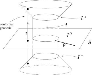
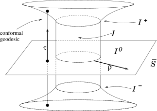
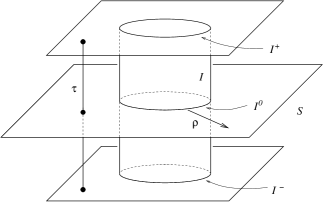
So far, the function $\kappa$ introduced in equation (1) has been required to be of the form $\kappa=\rho\kappa^{\prime}$, with $\kappa^{\prime}$ analytic an such that $\kappa^{\prime}(i)=1$, but otherwise it has remained unspecified . Two choices consistent with the requirement $\kappa=\rho\kappa^{\prime}$ will be considered here. The first, $\kappa=\rho$ is the simplest non-trivial one. For this choice ${I}^{+}$ in a neighbourhood of $I^{+}$ is concave, while ${I}^{-}$ in a neighbourhood of $I^{-}$ would be convex. The choice $\kappa=\rho$ has the virtue of rendering the simplest possible analytic expressions, both for the initial data (27a)-(27f) and the solution of the transport equations (37)-(40). Unfortunately, it is hard to attach to it some geometrical significance other that its simplicity. The other choice to be considered is $\kappa=\omega$. This choice is fine as under our assumptions $\omega=\rho+\mathcal{O}(\rho)$. With this choice,

$$\Theta=\omega^{-1}\Omega\left(1-\tau^{2}\right),$$ (45)

so that ${I}^{\pm}$ near $I^{\pm}$ are described by the hypersurfaces $\tau=\pm 1$, $\rho>0$ respectively: null infinity will be composed of two parallel planes, formally similar to the case of Minkowski —see [26] . Consequently, the system of conformal field equations (30)-(31) degenerate not only on $I^{\pm}$ but also on ${I}^{\pm}$. Thus, the choice $\kappa=\omega$ has more geometrical and analytic relevance. As a drawback it renders more complicated analytic expressions.

Figure 2: Effect of the choice of the function $\kappa$ on the representation of null infinity near spatial infinity. To the left with the choice $\kappa=\rho$; to the right the choice $\kappa=\omega$ so that null infinity corresponds to the hypersurfaces $\tau=\pm 1$.

For future use, we note the following result on the expansion types of the diverse unknowns appearing in the transport equations (37) and (40). Its proof comes from inspection [17].

Lemma 2.

The functions $\left(c^{1}_{ab}-\rho x_{ab}\right)^{(p)}$, $v^{(p)}$, $\phi^{(p)}$ $p=1,2,\dots$, are of expansion type $p-2$, $p-1$, and $p$ respectively.

4.1 A first analysis of the transport equations

A detailed first analysis of the structure of the solutions of the transport equations have been given in [17]. Because of its relevance for the purposes of the present article, and in order to fully motivate our later discussion, we briefly proceed to review it.

As seen in the previous section, the transport equations corresponding to the $v^{(p)}$ quantities, equation (37) are fully regular, thus in a first analysis one could just focus on the transport equations arising from the Bianchi identities, equation (40). The system can be written as,

$$(1+\tau)\partial_{\tau}\phi_{0}^{(p)}+X_{+}\phi_{1}^{(p)}-(p-2)\phi_{0}^{(p)}=R_{0}^{(p)},$$ (46a)

$$\partial_{\tau}\phi_{1}^{(p)}+\frac{1}{2}(X_{+}\phi_{2}^{(p)}+X_{-}\phi_{0}^{(p)})+\phi_{1}^{(p)}=R_{1}^{(p)},$$ (46b)

$$\partial_{\tau}\phi_{2}^{(p)}+\frac{1}{2}(X_{+}\phi_{3}^{(p)}+X_{-}\phi_{1}^{(p)})=R_{2}^{(p)},$$ (46c)

$$\partial_{\tau}\phi_{3}^{(p)}+\frac{1}{2}(X_{+}\phi_{4}^{(p)}+X_{-}\phi_{2}^{(p)})-\phi_{3}^{(p)}=R_{3}^{(p)},$$ (46d)

$$(1-\tau)\partial_{\tau}\phi_{4}^{(p)}+X_{-}\phi_{3}^{(p)}+(p-2)\phi_{4}^{(p)}=R_{4}^{(p)}.$$ (46e)

We will also make use of the transport equation arising from the Bianchi transport equations, equation (43). These we write as,

$$\tau\partial_{\tau}\phi_{1}^{(p)}+\frac{1}{2}(X_{+}\phi_{2}^{(p)}-X_{-}\phi_{0}^{(p)})-p\phi_{1}^{(p)}=S_{1}^{(p)},$$ (47a)

$$\tau\partial_{\tau}\phi_{2}^{(p)}+\frac{1}{2}(X_{+}\phi_{3}^{(p)}-X_{-}\phi_{1}^{(p)})-p\phi_{2}^{(p)}=S_{2}^{(p)},$$ (47b)

$$\tau\partial_{\tau}\phi_{3}^{(p)}+\frac{1}{2}(X_{+}\phi_{4}^{(p)}-X_{-}\phi_{2}^{(p)})-p\phi_{3}^{(p)}=S_{3}^{(p)}.$$ (47c)

The quantities $R^{(p)}_{j}$, $j=0,\ldots,4$ and $S^{(p)}_{i}$, $i=1,2,3$, are constructed from $v^{(k)}$ unknowns with $0\leq k\leq p$, and from $\phi^{(k)}$ quantities with $0\leq k\leq p-1$. All these quantities are assumed to be known. In this first analysis their detailed structure will no be crucial. It will suffice to know that they are of expansion type $p-1$. On the other hand, consequently with lemma 2 we write,

$$\phi^{(p)}_{j}=\sum_{q=|2-j|}^{p}\sum_{k=0}^{2q}a_{j,p;2q,k}T_{2q\phantom{k}q-2+j}^{\phantom{2q}k},$$ (48)

where the coefficients $a_{j,p;2q,k}=a_{j,p;2q,k}(\tau)$ are complex valued functions. The expression (48) effectively introduces a decomposition into spherical harmonics for the equations (46a)-(47c). In this way one has only to deal with ordinary differential equations. By taking linear combinations of equations (46b) and (47a), (46c) and (47b), (46d) and (47c) it can be readily seen that the coefficients $a_{1,p;2q,k}$, $a_{2,p;2q,k}$, $a_{3,p;2q,k}$ can be determined once the coefficients $a_{0,p;2q,k}$ and $a_{4,p;2q,k}$ are known. These last two coefficients can be seen to satisfy the following equations,

$$(1+\tau)f(\tau)a^{\prime}_{0,p;2q,k}+g(\tau)a_{0,p;2q,k}+h(\tau)a_{4,p;2q,k}=T_{0},$$ (49a)

$$-(1-\tau)f(-\tau)a^{\prime}_{4,p;2q,k}+g(-\tau)a_{4,p;2q,k}+h(\tau)a_{0,p;2q,k}=T_{4},$$ (49b)

where

$$f(\tau)=2(p+1)(p-1)-(q-1)(q+2)(1-\tau^{2}),$$

$$g(\tau)=-(p-2)f(\tau)+(q-1)(q+2)\left((p+1)(1+\tau)-(1+\tau)^{2}-\frac{1}{4p}q(q+1)(1-\tau)(1+\tau)^{2}\right),$$

$$h(\tau)=\frac{1}{4p}(q-1)q(q+1)(q+2)(1-\tau)^{3},$$

and $T_{0}$, $T_{4}$, depend on the coefficients $a_{j^{\prime},p^{\prime};q^{\prime},k^{\prime}}$ with $p<p^{\prime}$. They vanish, in particular, for $q=p$ as a consequence of $R^{(p)}_{j}$ and $S^{(p)}_{i}$ being of expansion type $p-1$. In order to solve the system (49a)-(49b), one can try to construct a fundamental matrix of the homogeneous system. Remarkably, the homogeneous versions of equations (49a) and (49b) can be decoupled to obtain two Jacobi equations (second order). This class of equations have been studied extensively in the literature.

For $0\leq q\leq p-1$ one gets for the system (49a)-(49b) a fundamental matrix,

$$X_{p;2q,k}=\left(\begin{array}[]{cc}\check{Q}_{p;2q,k}(\tau)&(-1)^{q}\hat{Q}_{p;2q,k}(\tau)\\ (-1)^{q}\hat{Q}_{p;2q,k}(-\tau)&\check{Q}_{p;2q,k}(-\tau)\\ \end{array}\right),$$ (50)

where

$$\check{Q}_{p;2q,k}(\tau)=\left(\frac{1-\tau}{2}\right)^{p+2}P_{q-2}^{(p+2,2-p)}(\tau),$$ (51)

and

$$\hat{Q}_{p;2q,k}(\tau)=\left(\frac{1+\tau}{2}\right)^{p-2}P_{q+2}^{(-p-2,p-2)}(\tau),$$ (52)

with $P_{n}^{(\alpha,\beta)}(\tau)$ the generalised Jacobi polynomials,

$$P_{n}^{(\alpha,\beta)}(\tau)=\sum_{\nu=0}^{n}\binom{n+\alpha}{n-\nu}\binom{n+\beta}{\nu}\left(\frac{\tau-1}{2}\right)^{\nu}\left(\frac{\tau+1}{2}\right)^{n-\nu}.$$ (53)

It is noted by passing that the fundamental matrix $X_{p;2q,k}$ for given $p$ and $q$ does not depend on $k$. If $p=q$ the story is other. In this case the fundamental matrix is of the form,

$$X_{p;2p,k}=\left(\begin{array}[]{cc}c_{11}\check{Q}_{p;2p,k}(\tau)&c_{12}\hat{Q}_{p;2p,k}(\tau)\\ c_{21}\hat{Q}_{p;2p,k}(-\tau)&c_{22}\check{Q}_{p;2p,k}(-\tau)\\ \end{array}\right),$$ (54)

where,

$$\check{Q}_{p;2p,k}(\tau)=\left(\frac{1-\tau}{2}\right)^{p+2}\left(\frac{1+\tau}{2}\right)^{p-2}$$ (55)

$$\hat{Q}_{p;2p,k}(\tau)=\int_{0}^{\tau}\frac{ds}{(1+s)^{p-1}(1-s)^{p+3}},$$ (56)

and $c_{11}$, $c_{12}$, $c_{21}$ and $c_{22}$ are numerical constants. A simple induction argument shows that,

$$\int_{0}^{\tau}\frac{ds}{(1+s)^{p-1}(1-s)^{p+3}}=A_{*}\ln(1-\tau)+\frac{A_{p+2}}{(1-\tau)^{p+2}}+\cdots+\frac{A_{1}}{(1-\tau)}+A_{0}$$

$$\phantom{\int_{0}^{\tau}\frac{ds}{(1+s)^{p-1}(1-s)^{p+3}}=}+B_{*}\ln(1+\tau)+\frac{B_{p-2}}{(1+\tau)^{p-2}}+\cdots+\frac{B_{1}}{(1+\tau)},$$

where the $A$’s and the $B$’s are some numerical coefficients. They precise values are not relevant for our purposes. It follows from the latter discussion that any solution for the sectors with $p=q$ will contain logarithmic divergences at $\tau=\pm 1$ unless $a_{0,p;2p,k}(0)=a_{4,p;2p,k}(0)$. Quite remarkably, for time symmetric initial data this quite involved and technical-looking condition can be reexpressed in terms of a very geometric and appealing condition on the Cotton-Bach tensor of the initial data at spatial infinity [17]. One has the following lemma:

Lemma 3.

For time symmetric initial data the following two conditions are equivalent,

• $$a_{0,p;2p,k}(0)=a_{4,p;2p,k}(0)$$ (57)

  with $p\geq 2$ and $k=0,\ldots,2p$,

• $$D_{(a_{s}b_{s}}\cdots D_{a_{1}b_{1}}b_{abcd)}(i)=0,$$ (58)

  with $s=0,1,\ldots$  .

From the above discussion it should be clear that the condition (58) is a necessary requirement in order to for the solutions $\phi_{j}^{(p)}$ of the transport equations (40) are smooth. Therefore we refer to condition (58) as to a regularity condition, and we have the following very suggestive result,

Theorem 1 (Friedrich, 1997).

The solutions $u^{(p)}$ of the transport equations extend smoothly to the sets $I^{\pm}$ only if the condition

$$D_{(a_{s}b_{s}}\cdots D_{a_{1}b_{1}}b_{abcd)}(i)=0,\quad s=0,1,\ldots$$

is satisfied at all orders $s$. It is is not satisfied for some $s$, the solution develops logarithmic singularities at $I^{\pm}$.

It should be emphasized that the consideration leading to this last theorem have hardly make use of the inhomogeneous terms of equations (49a) and (49b). The system (49a)-(49b) can be in matricial form as,

$$A_{p;2q}(\tau)y^{\prime}_{p;2q,k}(\tau)+B(\tau)y_{p;2q,k}(\tau)=t_{p;2q,k},$$ (59)

where $A_{p;2q}$ and $B_{p;2q}$ are $2\times 2$, and $t_{p;2q,k}$ is a column vector such that $t_{p;2p,k}=0$. The the solution of system given in terms of the fundamental matrix is then,

$$y_{p;2q,k}(\tau)=X_{p;2q,k}(\tau)X^{-1}_{p;2q,k}(0)y_{p;2q,k}(0)+\int_{0}^{\tau}X_{p;2q,k}^{-1}(s)\;A_{p;2q}^{-1}(s)\;t_{p;2q,k}(s)ds.$$ (60)

Assume that the regularity condition (58) holds. Even in this case the integrand $X^{-1}_{p;2q}(\tau)A^{-1}_{p;2q}(\tau)\;t_{p;2q,k}(\tau)$ in formula (60) contains poles at $\tau=\pm 1$ and possibly also outside the interval $[-1,1]$. Therefore, unless some remarkable property of the conformal field equations comes into stage, the solution vector $y_{p;2q,k}$ will contain some logarithmic terms and consequently also the coefficients $\phi_{j}^{(p)}$.

The algebraic structure of the integral in (60) is too complicated to analyse directly without resorting to some further (still unknown) structure of the field equations. In order to shed some light into this direction, Friedrich & Kánnár have performed an analysis of the solutions of the transport equations up to order $p=3$ under the assumption that the initial data satisfies the condition (58). Quite remarkably they found that no logarithms appeared in the solutions. This meant that somehow, the simple poles in (60) cancel out up to the order under consideration.

At this point it is important to mention that due to the gauge conditions used in the whole construction, we know that the logarithmic singularities occurring in the solutions to the transport equations are associated with the conformal structure, and are not artifacts of a choice of gauge. Note that the condition equation (58) is conformally invariant. It allows us to identify obstructions to the smoothness of null infinity explicitly in terms of the initial data. Also, because of the hyperbolic nature of the equations suggest that if logarithmic terms are present in the solutions of the transport equations, then it is very likely these will propagate along ${I}$.

5 Solving the transport equations given time symmetric, conformally flat initial data

On simplicity and aesthetical grounds it is natural to wonder whether the regularity condition, equation (58), is the only requirement one has to impose on the initial data in order to obtain solutions to the transport equations which are smooth —see for example the discussion in [19]. Before trying to prove some statement along this lines, it is of clear interest to calculate the some further order in the expansions. The rationale behind it being firstly to verify whether the conjecture still holds, and secondly to try to find some patterns in the solutions that one could exploit in an eventual abstract proof. In order to simplify the calculations, we have chosen to restrict our attention to those time symmetric initial data sets which are conformally flat. These satisfy the regularity condition (58) in a trivial way. Thus, they represent the simplest (non-trivial) class of initial data sets one can look at. Their simplicity is somehow deceiving, and should not be regarded as a drawback on the kind of insight that can be gained through them. A great deal about the solutions of the Einstein field equations has been learned from the analysis of this class of initial data —see e.g. [1, 21, 27].

The already “big” transport equation systems (37)-(40) do not give an appropriate dimension of the computational difficulties one has to face if one is to take the expansions carried in [20] to even higher orders. However, the calculations one has to carry are suitable to a treatment using a computer algebra system. In order to analyse with ease the solutions of the transport equations some scripts in the computer algebra system Maple V have been written. The reader is remitted to the appendix for further details on the implementation of the calculations on this system.

Because of the largeness of the expressions contained inthe solutions, we have opted to provide a description of the qualitative features of the expansions rather than a complete list of all the terms calculated. In particular, attention will be focused on the solutions to the transport equations arising from the Bianchi identities, the functions $\phi_{j}^{(p)}$. It should be emphasized that this does not mean that the solutions to the $v$ unknown transport equations are not important. They are also crucial: a tiny mistake in the calculation of their solutions would destroy the whole structure of the solutions. However, as the discussion in the previous section has pointed out, the logarithmic terms that destroy the smoothness of null infinity appear firstly in the components of the Weyl spinor.

In order to perform our expansions a number of assumptions have been made. We list them here for the purposes of a quick reference.

Assumptions.

It will be assumed that:

• the initial data set is asymptotically Euclidean and time symmetric.

• in a neighbourhood $B_{a}(i)$ of $i$ the initial data is assumed to be conformally flat. The function $W$ appearing in the conformal factor of the initial hypersurface —see equation (24)— is a solution of the Laplace equation admitting in $B_{a}(i)$ a decomposition of the form,

  $$W=\frac{1}{2}m+\sum_{i=1}^{8}\frac{1}{i!}W_{i}\rho^{i}+\mathcal{O}(\rho^{9}),$$ (61)

  where

  $$W_{i}=\sum_{k=0}^{2i}w_{i,2i,k}T_{2i\phantom{k}i}^{\phantom{2i}k},$$ (62)

  with the coefficients $w_{i,2i,k}$, $i=1,\ldots,7$, $k=0,\dots,2i$ complex numbers satisfying $\overline{w}_{i,2i,k}=(-1)^{i+k}w_{i,2i,2i-k}$ so that $W$ is a real valued function. This is in consistency with the decomposition given in equation (25).

• Likewise, the components of the vector unknowns $v^{(p)}$ and $\phi^{(p)}$ admit on $I$ expansions in terms of $T_{j\phantom{k}l}^{\phantom{j}k}$ functions consistent with lemma 2.

• The two following choices of the function $\kappa$ —see equation (1)— will be considered:

  $$\kappa_{1}=\rho,$$

  $$\kappa_{2}=\omega.$$

The result of the calculations under these assumptions are now described.

5.1 The orders $p=0,\ldots,4$.

Firstly, calculations for the orders $p=1$, $p=2$ and $p=3$ were undertaken. The results are in complete agreement with those given by Friedrich & Kánnár when reduced to the case of conformally flat initial data.

The solutions at order $p=0$ can be schematically written as,

$$\phi_{0}^{(0)}=0,$$ (63a)

$$\phi_{1}^{(0)}=0,$$ (63b)

$$\phi_{2}^{(0)}=-m,$$ (63c)

$$\phi_{3}^{(0)}=0,$$ (63d)

$$\phi_{4}^{(0)}=0.$$ (63e)

independently of the choice of $\kappa$. At order $p=1$ one has,

$$\phi_{0}^{(1)}=0,$$ (64a)

$$\phi_{1}^{(1)}=-3\,X_{+}W_{1}(1-\tau)^{2},$$ (64b)

$$\phi_{2}^{(1)}=m^{2}(\frac{1}{2}\tau^{4}-3\tau^{2})+6\,W_{1}(\tau^{2}-1)$$ (64c)

$$\phi_{3}^{(1)}=3\,X_{-}W_{1}(1+\tau)^{2},$$ (64d)

$$\phi_{4}^{(1)}=0.$$ (64e)

when $$\kappa=\rho \phi_{0}^{(1)} \phi_{1}^{(1)} \phi_{3}^{(1)} \phi_{4}^{(1)} \kappa=\omega \phi_{2}^{(1)}$$. The expressions for , , and for the choice are similar. That of is given by,

$$\phi_{2}^{(1)}=m^{2}(\frac{1}{2}\tau^{4}-3\tau^{2}-\frac{3}{2})+6\,W_{1}(\tau^{2}-1).$$ (64f)

At order $p=2$ one has,

$$\phi_{0}^{(2)}=f_{1}(\tau)X_{+}X_{+}W_{2},$$ (65a)

$$\phi_{1}^{(2)}=f_{2}(\tau)mX_{+}W_{1}+f_{3}(\tau)X_{+}W_{2},$$ (65b)

$$\phi_{2}^{(2)}=f_{4}(\tau)m^{3}+f_{5}(\tau)mW_{1}+f_{6}(\tau)W_{2},$$ (65c)

$$\phi_{3}^{(2)}=-f_{2}(-\tau)mX_{-}W_{1}-f_{3}(-\tau)X_{-}W_{2},$$ (65d)

$$\phi_{4}^{(2)}=f_{1}(-\tau)X_{-}X_{-}W_{2},$$ (65e)

where $f_{i}(\tau)$, $i=1,\ldots 6$ are polynomials on $\tau$. Their explicit form is not relevant for our purposes. The polynomials are slightly different for each of the choices of $\kappa$, but of the same order. Similarly, the components of the Weyl tensor at order $p=3$ are of the form,

$$\phi_{0}^{(3)}=g_{1}(\tau)X_{+}X_{+}W_{3}+g_{2}(\tau)mX_{+}X_{+}W_{2}+g_{3}(\tau)(X_{+}W_{1})^{2},$$ (66a)

$$\phi_{1}^{(3)}=g_{4}(\tau)X_{+}W_{3}+g_{5}(\tau)mX_{+}W_{2}+g_{6}(\tau)W_{1}X_{+}W_{1}+g_{7}(\tau)m^{2}X_{+}W_{1},$$ (66b)

$$\phi_{2}^{(3)}=g_{8}(\tau)W_{3}+g_{9}(\tau)mW_{2}+g_{10}(\tau)(W_{1})^{2}+g_{11}(\tau)^{2}m^{2}W_{1}+g_{12}(\tau)m^{4}+g_{13}(\tau)b,$$ (66c)

$$\phi_{3}^{(3)}=-g_{4}(-\tau)X_{-}W_{3}-g_{5}(-\tau)mX_{-}W_{2}-g_{6}(-\tau)W_{1}X_{-}W_{1}-g_{7}(-\tau)m^{2}X_{-}W_{1},$$ (66d)

$$\phi_{4}^{(3)}=g_{1}(-\tau)X_{-}X_{-}W_{3}+g_{2}(-\tau)mX_{-}X_{-}W_{2}+g_{3}(-\tau)(X_{-}W_{1})^{2}.$$ (66e)

Again, the functions $g_{i}(\tau)$, $i=1,\ldots,13$ are polynomials, while $b=2w_{1,2,0}w_{1,2,2}-w_{1,2,1}^{2}$ is a constant.

The first new order corresponds to $p=4$. Here, again, the solutions are still fully regular and polynomial:

$$\phi_{0}^{(4)}=h_{1}(\tau)X_{+}W_{1}X_{+}W_{2}+h_{2}(\tau)W_{1}X_{+}X_{+}W_{2}+h_{3}(\tau)m(X_{+}W_{1})^{2}$$

$$\phantom{XXXXXXXX}+h_{4}(\tau)mX_{+}X_{+}W_{3}+h_{5}(\tau)X_{+}X_{+}W_{4},$$ (67a)

$$\phi_{1}^{(4)}=h_{6}(\tau)m^{3}X_{+}W_{1}+h_{7}(\tau)W_{2}X_{+}W_{1}+h_{8}(\tau)W_{1}X_{+}W_{2}+h_{9}(\tau)mW_{1}X_{+}W_{1}$$

$$\phantom{XXXXXXXX}+h_{10}(\tau)mX_{+}W_{3}+h_{11}(\tau)X_{+}W_{4},$$ (67b)

$$\phi_{2}^{(4)}=h_{12}(\tau)m^{5}+h_{13}(\tau)b+h_{14}(\tau)m^{3}W_{1}+h_{15}(\tau)W_{1}W_{2}+h_{16}(\tau)m(W_{1})^{2}$$

$$\phantom{XXXXXXXX}+h_{17}(\tau)mW_{3}+h_{18}(\tau)W_{4},$$ (67c)

$$\phi_{3}^{(4)}=-h_{6}(-\tau)m^{3}X_{-}W_{1}-h_{7}(-\tau)W_{2}X_{-}W_{1}-h_{8}(-\tau)W_{1}X_{-}W_{2}-h_{9}(-\tau)mW_{1}X_{-}W_{1}$$

$$\phantom{XXXXXXXX}-h_{10}(-\tau)mX_{-}W_{3}-h_{11}(-\tau)X_{-}W_{4},$$ (67d)

$$\phi_{4}^{(4)}=h_{1}(-\tau)X_{-}W_{1}X_{-}W_{2}+h_{2}(-\tau)W_{1}X_{-}X_{-}W_{2}+h_{3}(-\tau)m(X_{-}W_{1})^{2}$$

$$\phantom{XXXXXXXX}+h_{4}(-\tau)mX_{-}X_{-}W_{3}+h_{5}(-\tau)X_{-}X_{-}W_{4}.$$ (67e)

Again, the functions $h_{i}(\tau)$, $i=1,\ldots,16$ are polynomials.

5.2 The first obstructions to smoothness: orders $p=5,6$.

The calculation of the solutions to the Bianchi transport equations up to order $p=4$ have shown that all of them are polynomial, and thus smooth at $I^{\pm}$. Consequently, the $v$ unknowns also happen to be polynomial. The first modifications to this behaviour occur at the rather high order $p=5$. Feeding the solution of the transport equations up to order $p=4$ into the $v$ transport equations (37) with $p=5$ and solving one finds again that the components of $v^{(5)}$ are again polynomial. However, the solution of the Bianchi transport equations are of the form,

$$\phi_{0}^{(5)}=C_{0}m^{2}G^{(5)}\Bigl{(}(1-\tau)^{7}\ln(1-\tau)$$

$$\phantom{XXXXXX}+(1+\tau)^{3}(351-150\tau+48\tau^{2}-10\tau^{3}+\tau^{4})\ln(1+\tau)\Bigr{)}+k_{0}(\tau),$$ (68a)

$$\phi_{1}^{(5)}=C_{1}m^{2}G^{(5)}\Bigl{(}(1-\tau)^{6}(2\tau+5)\ln(1-\tau)$$

$$\phantom{XXXXXX}-(2\tau^{3}-15\tau^{2}+48\tau-75)(1+\tau)^{4}\ln(1+\tau)\Bigr{)}+k_{1}(\tau),$$ (68b)

$$\phi_{2}^{(5)}=C_{2}m^{2}G^{(5)}\Bigl{(}(1-\tau)^{5}(\tau^{2}+5\tau+8)\ln(1-\tau)$$

$$\phantom{XXXXXX}+(1+\tau)^{5}(\tau^{2}-5\tau+8)\ln(1+\tau)\Bigr{)}+k_{2}(\tau),$$ (68c)

$$\phi_{3}^{(5)}=C_{1}m^{2}G^{(5)}\Bigl{(}(1-\tau)^{4}(2\tau^{3}+15\tau^{2}+48\tau+75)\ln(1-\tau)$$

$$\phantom{XXXXXX}-(1+\tau)^{6}(2\tau-5)\ln(1+\tau)\Bigr{)}+k_{3}(\tau),$$ (68d)

$$\phi_{4}^{(5)}=C_{0}m^{2}G^{(5)}\Bigl{(}(1-\tau)^{3}(351+150\tau+48\tau^{2}+10\tau^{3}+\tau^{4})\ln(1-\tau)$$

$$\phantom{XXXXXX}+(1+\tau)^{7}\ln(1+\tau)\Bigr{)}+k_{4}(\tau),$$ (68e)

where $C_{0}$, $C_{1}$, $C_{3}$ are non-relevant non-zero numerical factors, $k_{i}(\tau)$ $i=0,\ldots,4$ are polynomials analogous to, for example, those in (67a)-(67e), depending on $m$, $W_{1}$, $W_{2}$, $W_{3}$, $W_{4}$, their $X_{\pm}$ derivatives and products of them. Most remarkably,

$$G^{(5)}=\sum_{k=0}^{4}G^{(5)}_{k}T_{4\phantom{k}2}^{\phantom{4}k},$$ (69)

where,

$$G^{(5)}_{0}=mw_{2,4,0}-2\sqrt{6}w_{1,2,0}^{2},$$ (70a)

$$G^{(5)}_{1}=mw_{2,4,1}-4\sqrt{3}w_{1,2,0}w_{1,2,1},$$ (70b)

$$G^{(5)}_{2}=mw_{2,4,2}-4w_{1,2,1}^{2}-4w_{1,2,0}w_{1,2,2},$$ (70c)

$$G^{(5)}_{3}=mw_{2,4,3}-4\sqrt{3}w_{1,2,1}w_{1,2,2},$$ (70d)

$$G^{(5)}_{4}=mw_{2,4,4}-2\sqrt{6}w_{1,2,2}^{2}.$$ (70e)

Thus, the coefficients $G^{(5)}_{k}$ are (besides an irrelevant numerical factor) the Newman-Penrose constants of the development of the time symmetric conformally flat initial data —[20].

Plugging the solutions (68a)-(68e) into the transport equations for $p=6$ one finds that the solutions of the sectors of the form $T_{4\phantom{k}j}^{\phantom{4}k}$ develop terms containing $\ln^{2}(1-\tau)$ and $\ln(1-\tau)$. Furthermore, the sectors $T_{6\phantom{k}j+1}^{\phantom{6}k}$ in $\phi^{(p)}_{j}$ contain logarithms. More precisely, the solution will be of the form,

$$\phi_{j}^{(6)}=G^{(5)}\Bigl{(}l_{1_{j}}(\tau)\ln^{2}(1-\tau)+l_{2_{j}}(\tau)\ln(1-\tau)+l_{3_{j}}(\tau)\ln^{2}(1+\tau)+l_{4_{j}}(\tau)\ln(1+\tau)\Bigr{)}$$

$$\phantom{XXXXX}+G^{(6)}\Bigl{(}l_{5_{j}}(\tau)\ln(1-\tau)+l_{6_{j}}(\tau)\ln(1+\tau)\Bigr{)}+l_{7_{j}}(\tau),$$ (71)

where $j=0,\ldots,7$, and $l_{k_{j}}(\tau)$ are polynomials. The coefficients $G^{(6)}$ are new obstructions to the smoothness of the solutions. These will be discussed a bit later. It is not hard to imagine that from this point onwards, terms containing $\ln(1-\tau)$, $\ln(1+\tau)$ and higher order powers of them will spread all around the solutions to the transport equations. Instead of analysing this phenomenon, we will rather focus on the smooth solutions.

Setting the Newman-Penrose constants to zero, the solution at order $p=6$ is of the form,

$$\phi_{0}^{(6)}=D_{0}m^{3}G^{(6)}\Bigl{(}(2+\tau)(1-\tau)^{8}\ln(1-\tau)$$

$$\phantom{XXXX}+(-254+233\tau-128\tau^{2}+46\tau^{3}-10\tau^{4}+\tau^{5})(1+\tau)^{4}\ln(1+\tau)\Bigr{)}+l_{0}(\tau),$$ (72a)

$$\phi_{1}^{(6)}=D_{1}m^{3}G^{(6)}\Bigl{(}(23+20\tau+5\tau^{2})(1-\tau)^{7}\ln(1-\tau)$$

$$\phantom{XXXX}-(233-256\tau+138\tau^{2}-40\tau^{3}+5\tau^{4})(1+\tau)^{5}\ln(1+\tau)\Bigr{)}+l_{1}(\tau),$$ (72b)

$$\phi_{2}^{(6)}=D_{2}m^{3}G^{(6)}\Bigl{(}(64+69\tau+30\tau^{2}+5\tau^{3})(1-\tau)^{6}\ln(1-\tau)$$

$$\phantom{XXXX}+(-64+69\tau)-30\tau^{2}-5\tau^{3})(1+\tau)^{6}\ln(1+\tau)\Bigr{)}+l_{2}(\tau),$$ (72c)

$$\phi_{3}^{(6)}=D_{1}m^{3}G^{(6)}\Bigl{(}(233+256\tau+138\tau^{2}+40\tau^{3}+5\tau^{4})(1-\tau)^{5}\ln(1-\tau)$$

$$\phantom{XXXX}+(23-20\tau+5\tau^{2})(1+\tau)^{7}\ln(1+\tau)\Bigr{)}+l_{3}(\tau),$$ (72d)

$$\phi_{4}^{(6)}=D_{0}m^{3}G^{(6)}\Bigl{(}(254+233\tau+128\tau^{2}+46\tau^{3}+10\tau^{4}+\tau^{5})(1-\tau)^{4}\ln(1-\tau)$$

$$\phantom{XXXX}+(-2+\tau)(1+\tau)^{8}\ln(1+\tau)\Bigr{)}+l_{4}(\tau),$$ (72e)

with $l_{0}(\tau),\dots,l_{4}(\tau)$ polynomials, and

$$G^{(6)}=\sum_{k=0}^{6}G^{(6)}_{k}T_{6\phantom{k}3}^{\phantom{6}k},$$ (73)

where the coefficients $G^{(6)}_{k}$, $k=0,\dots,6$ are given in terms of initial data quantities by,

$$G^{(6)}_{0}=m^{2}w_{3,6,0}-12\sqrt{10}w_{1,2,0}^{3},$$ (74a)

$$G^{(6)}_{1}=m^{2}w_{3,6,1}-12\sqrt{30}w_{1,2,0}^{2}w_{1,2,1},$$ (74b)

$$G^{(6)}_{2}=m^{2}w_{3,6,2}-24\sqrt{6}w_{1,2,0}w_{1,2,1}^{2}-12\sqrt{6}w_{1,2,0}^{2}w_{1,2,2},$$ (74c)

$$G^{(6)}_{3}=m^{2}w_{3,6,3}-72w_{1,2,0}w_{1,2,1}w_{1,2,2}-24w_{1,2,1}^{3},$$ (74d)

$$G^{(6)}_{4}=m^{2}w_{3,6,4}-24\sqrt{6}w_{1,2,1}^{2}w_{1,2,2}-12\sqrt{6}w_{1,2,0}w_{1,2,2}^{2},$$ (74e)

$$G^{(6)}_{5}=m^{2}w_{3,6,5}-12\sqrt{30}w_{1,2,1}w_{1,2,2}^{2},$$ (74f)

$$G^{(6)}_{6}=m^{2}w_{3,6,6}-12\sqrt{10}w_{1,2,2}^{3}.$$ (74g)

In analogy to the order $p=5$ we will refer to these coefficients as to the order $6$ Newman-Penrose “constants”. One is naturally bound to ask whether the coefficients $G^{(6)}$ are actually associated to some conserved quantities at null infinity in the same way that the coefficients $G^{(5)}$ are. This consideration is beyond the scope of the present article, and will be analysed in detail in future work. It is pointed out, as a plausibility argument, that in the analysis of polyhomogeneous Bondi expansions carried out in for example [3, 24, 25], the first logarithmic terms appearing in the expansions were associated with a conserved quantity on null infinity. As it can be seen from our discussion, if $G^{(5)}=0$, then the first logarithmic terms appearing in our expansions are precisely those associated to $G^{(6)}$. Notwithstanding, the expansions described here are based in the conformal geodesics gauge, while those in [3, 24, 25] use the so-called Bondi gauge. Thus, one would have to look in detail the possible appearance of logarithmic terms in the transformation connecting the two gauges.

Theorem (Main theorem, precise formulation).

Necessary conditions for the development of initial data which is time symmetric and conformally flat in a neighbourhood $B_{a}(i)$ of (spatial) infinity to be smooth on the set $I\cup I^{+}\cup I^{-}$ are that the Newman-Penrose constants, $G^{(5)}_{k}$, $k=0,\ldots,5$, should vanish. Furthermore, the “higher order” Newman-Penrose constants, $G^{(6)}_{k}$, $k=0,\ldots,6$, should also vanish. If only the coefficients $G^{(5)}_{k}$ vanish then the rescaled Weyl spinor is at most $C^{2}$ on a neighbourhood of either $I^{+}$ or $I^{-}$. If both $G^{(5)}$ and $G^{(6)}$ vanish then generically the Weyl tensor will be at most of class $C^{3}$ of the latter neighbourhoods.

From the last result one can extract directly the following (important) consequence:

Corollary 1.

The regularity condition (58) is not a sufficient condition for the smoothness at $I\cup I^{+}\cup I^{-}$ of the development of asymptotically Euclidean, time symmetric initial data sets.

This corollary is, thus, a negative answer to the conjecture raised in [19]. It is nevertheless surprising that the obstructions to the smoothness of null infinity arise at such a high order in the expansions. In order to acquire a deeper understanding of why this is the case would require in turn an abstract understanding of the algebraic structure of the transport equations (37) and (40). It is not unreasonable to reckon that some group theoretical properties of the whole set up play a major role here.

The theorem also suggest the following un expected conjecture:

Conjecture.

The developments of the Brill-Lindquist and Misner initial data sets possess non-smooth null infinities.

In [9, 27] the Newman-Penrose constants of the Brill-Lindquist and Misner data sets [1, 21] have been calculated using the formula found by Friedrich & Kánnár [20]. Due to the axial symmetry, there is only one non-vanishing Newman-Penrose constant. Furthermore, the constant vanishes if and only if the data sets are actually the Schwarzschild initial data. That the development of these two initial data sets possess a non-smooth null infinity may have implications in the description of their late time behaviour in terms of linear perturbations on a Schwarzschild background.

Some remarks regarding the theorem come also into place:

Remark 1. The calculations for the order $p=7$ are already beyond the capabilities of Maple V —the expressions involved are too large for the simplification routines of the computer algebra system, even for an Origin computer available at the Albert Einstein Institute. Nevertheless, the calculations of axially symmetric situations are still possible. These have been carried out for the orders $p=7$ and $p=8$ inclusive. Assuming that both $G^{(5)}$ and $G^{(6)}$ vanish, the solutions of the Bianchi transport equations have again the expected form:

$$\phi_{j}^{(7)}=E_{j}m^{3}G^{(7)}\Bigl{(}m_{1_{j}}(\tau)\ln(1-\tau)+m_{2_{j}}(\tau)\Bigr{)}+m_{3_{j}}(\tau),$$ (75)

where now due to the axial symmetry there is only one order $7$ Newman-Penrose constant,

$$G^{(7)}=\Bigl{(}m^{3}w_{4,8,4}-192w_{1,2,1}^{4}\Bigl{)}T_{8\phantom{4}4}^{\phantom{8}4}.$$ (76)

If in turn $G^{(7)}$ vanishes,

$$\phi_{j}^{(8)}=F_{j}m^{4}G^{(8)}\Bigl{(}n_{1_{j}}(\tau)\ln(1-\tau)+n_{2_{j}}(\tau)\Bigr{)}+n_{3_{j}}(\tau),$$ (77)

with,

$$G^{(8)}=\Bigl{(}m^{4}w_{5,10,5}-1920w_{1,2,1}^{5}\Bigl{)}T_{10\phantom{5}5}^{\phantom{10}5}.$$ (78)

From this evidence it is not too hard to guess the following general formula for the obstructions of the smoothness of null infinity in the axial situation,

$$G^{(p)}=\Bigl{(}m^{p-4}w_{p-3,2p-6,p-3}-2^{p-4}(p-4)!(w_{1,2,1})^{p-3}\Bigl{)}T_{2p-6\phantom{p-3}p-3}^{\phantom{2p-6}p-3}.$$ (79)

The proof of such a formula is nevertheless beyond our current understanding of the transport equations. The significance of the latter expression will be discussed in short.

Remark 2. In the non-axially symmetric case, it is conjectured that obstructions to the smoothness of null infinity (Generalised Newman-Penrose constants) are given in terms of the initial data by the following expressions,

$$G^{(p)}_{k}=m^{p-4}w_{p-3,2p-6,k}-\sum_{s_{0}+s_{1}+s_{2}=k}c_{p,k;s_{0},s_{1},s_{2}}w_{1,2,0}^{s_{0}}w_{1,2,1}^{s_{1}}w_{1,2,2}^{s_{2}},$$ (80)

with $k=0,1,\dots,p$, where the coefficients $c_{p,k;s_{0},s_{1},s_{2}}$ are some numerical constants.

5.3 Obstructions to smoothness and the Schwarzschild initial data.

As mentioned before, the Newman-Penrose constants of the Schwarzschild spacetime are all zero. Thus, in order to gain some insight into the significance of the expressions (79) and (80) it is convenient to see what occurs in the case of the Schwarzschild initial data.

It is not complicate —although certainly messy— to calculate an expression for initial data for the Schwarzschild on the slice of time symmetry. On this slice the initial 3-metric is conformally flat. Thus, the required (harmonic) conformal factor can be calculated directly from the Green function for the three dimensional Laplace equation in spherical coordinates. The Green function is given by,

$$G(r,\theta,\phi;r^{\prime},\theta^{\prime},\phi^{\prime})=\sum_{n=0}^{\infty}\sum_{m=-n}^{n}\frac{4\pi}{2n+1}\overline{Y_{n,m}(\theta,\phi)}Y_{n,m}(\theta^{\prime},\phi^{\prime})\frac{r^{\prime n}}{r^{n+1}},$$ (81)

for $r>r^{\prime}$.

The latter expression can be lifted into the frame bundle $C_{a,\kappa}$ and written in terms of the functions $T_{j\phantom{k}l}^{\phantom{j}k}$ using formula (15) to get,

$$W=\frac{m}{2}\sum_{n=0}^{\infty}\sum_{k=0}^{2n}r^{\prime n}T_{2n\phantom{2n-k}n}^{\phantom{2n}2n-k}(t^{\prime})\;T_{2n\phantom{k}n}^{\phantom{2n}k}\rho^{n}.$$ (82)

where $(t^{\prime},r^{\prime})$ denote the coordinates of the singularity of the Green function on the frame bundle. Thus, the $T_{2n\phantom{2n-k}n}^{\phantom{2n}2n-k}(t^{\prime})$ are fixed complex numbers. We write,

$$w_{n,2n,k}=\frac{1}{2}mr^{\prime n}n!T_{2n\phantom{2n-k}n}^{\phantom{2n}2n-k}(t^{\prime}),$$ (83)

for $n=0,1,\ldots$ and $k=0,\ldots,2n$. The latter coefficients are not independent but related to each other via recurrence relations, like

$$(n+1)(2n+1)w_{1,2,1}\times w_{n,2n,k}=\sqrt{(k+1)(2n-k+1)}w_{n+1,2(n+1),k+1}$$

$$\phantom{XXXXXXX}+r^{\prime 2}n(n+1)\sqrt{k(2n-k)}w_{n-1,2(n-1),k-1}.$$ (84)

These can be readily obtained from similar recurrence relations holding for the spherical harmonics. The Schwarzschild solution has an obvious axial symmetry. If one considers an orientation of the coordinate system in a way that makes this symmetry of the initial data explicit —the singularity of the Green function is set along the $z$ axis— one ends up with a much simplified expression,

$$W=\sum_{n=0}^{\infty}\left(\frac{2}{m}\right)^{n-1}(w_{1,2,1})^{n}T_{2n\phantom{n}n}^{\phantom{2n}n}\rho^{n},$$ (85)

so that the only non-vanishing $w_{n,2n,k}$ coefficients are given by,

$$w_{n,2n,n}=\left(\frac{2}{m}\right)^{n-1}(w_{1,2,1})^{n}n!\;.$$ (86)

One obtains precisely this expression if one requires that the hierarchy of axial Newman-Penrose constants, formula (79), vanishes at every order $p$. It is however important to point out that this is not a proof but again a plausibility argument as formula (79) has only been verified up to order $p=8$. A much more involved calculation shows that the expressions one obtains for the coefficients $w_{2,4,0},\ldots,w_{2,4,4}$ and $w_{3,6,0},\ldots,w_{3,6,6}$ by setting $G^{(5)}$ and $G^{(6)}$ to zero are precisely those one has for the Schwarzschild initial data. This involves the use of the recurrence relation (84).

Now, the fuction $W$ is a solution to $\Delta W=0$, and thus analytic. This in turn implies that the function $W$ one deduces from requiring the coefficients (79) to vanish at all orders $p$ is exactly Schwarzschildean. This evidence leads to the following,

Conjecture (Precise formulation).

For every $k>0$ there exists a $p=p(k)$ such that the time evolution of an asymptotically Euclidean, time symmetric, conformal flat, conformally smooth initial data set admits a conformal extension to null infinity of class $C^{k}$ near spacelike infinity, if and only if the initial data set is Schwarzschildean to order $p(k)$.

The latter is the successor of the conjecture, in the context of time symmetric conformally flat, of the conjecture by Friedrich [19] to which reference was made in the introduction.

6 Conclusions and extensions

The results presented in the main theorem together with the considerations leading to the conjecture put forward in section 5 seem to suggest that no gravitational radiation should be present around spatial infinity if one is to have a smooth null infinity. In other words, the notion of smooth null infinity seems to be incompatible with the presence of radiation around $i^{0}$. Whether this behaviour of spacetime in the neighbourhood of spatial infinity has some implications on either the demeanour of the sources of the gravitational field in the infinite past or on the nature of incoming radiation travelling from past null infinity is a naturally arising question.

A natural extension of the calculations here described would be to consider what happens with more general (i.e. not conformally flat) time symmetric initial data. If the time symmetric initial data is not conformally flat, then the Newman-Penrose constants are given in terms of the initial data by,

$$\widetilde{G}^{(5)}_{0}=mw_{2,4,0}-2\sqrt{6}w_{1,2,0}^{2}-\frac{1}{254\sqrt{6}}R^{(2)}_{0},$$

$$\widetilde{G}^{(5)}_{1}=mw_{2,4,1}-4\sqrt{3}w_{1,2,0}w_{1,2,1}-\frac{1}{254\sqrt{6}}R_{1}^{(2)},$$

$$\widetilde{G}^{(5)}_{2}=mw_{2,4,2}-4w_{1,2,1}^{2}-4w_{1,2,0}w_{1,2,2}-\frac{1}{254\sqrt{6}}R_{2}^{(2)},$$

$$\widetilde{G}^{(5)}_{3}=mw_{2,4,3}-4\sqrt{3}w_{1,2,1}w_{1,2,2}-\frac{1}{254\sqrt{6}}R_{3}^{(2)},$$

$$\widetilde{G}^{(5)}_{4}=mw_{2,4,4}-2\sqrt{6}w_{1,2,2}^{2}-\frac{1}{254\sqrt{6}}R_{4}^{(2)},$$

where $R_{k}^{(2)}$ are coefficients appearing in the expansion of the Ricci scalar $r$ of the initial $3$-metric, around spatial infinity. In the view of the present results one would expect to have the quantities $\widetilde{G}^{(5)}_{k}$ appearing as obstructions to the smoothness of null infinity. Similarly, one would expect to obtain generalisations $\widetilde{G}^{(6)}_{k}$ of the higher order Newman-Penrose constants $G^{(6)}_{k}$ by adding suitable expressions containing the Ricci scalar. Ultimately, one would like to prove that there is an infinite hierarchy of such quantities as obstructions to the smoothness of ${I}$. The relation of these quantities with static initial data is to be analysed, at least for the first orders. It could well be the case that a time symmetric initial data set will yield a development with smooth null infinity only if it is static in a neighbourhood of spatial infinity. In relation to this, it is noted that the asymptotically Euclidean static initial data satisfy the regularity condition (58) —see [16].

With regard to a proof to the conjecture presented in this article, it is noted that it would require a much deeper understanding of the properties of the transport equations at spatial infinity that the one currently available. In particular one would like to be able to discuss its algebraic properties in a much more abstract way, and with out having to resort to “explicit expressions” as it was done here. As mentioned before, group theoretical properties of the set up should play a crucial role here.

Acknowledgements

I thank H. Friedrich who suggested the problem and helped with discussions and clarifications all along the long winding road. I also thank S. Dain and M. Mars from which I have benefited through several discussions.

Appendix: on the Computer Algebra implementation

The calculations described in this article are hefty, however quite amenable to the use of computer algebra systems. In the present case the computer algebra system Maple V was used. The main source of difficulties in solving the transport equations implied by the conformal field equation on the cylinder at spatial infinity is not the actual procedure of solving the equations, but producing the equations that have to be solved. To understand why this is the case, we recall the quasilinear nature of the transport equations. Accordingly, in the construction of the equations for the diverse spherical sectors of the various unknowns one encounters products of the functions $T_{j\phantom{k}l}^{\phantom{j}k}$, which have to be expanded using the formula (19), which in turn requires the computation of several Clebsch-Gordan coefficients. The number of these products heavily increases as one considers higher and higher expansions orders. There are Maple V scripts available in the web. We have made use of those written by A. B. Coates [4].

For the purposes of the computer algebra implementation, the diverse spinor arising have been considered as arrays running on the set of indices $\{0,1\}$. In this way all the elementary spinors introduced in section 2.1 can be readily defined. For example, the spinor $x_{ab}$ would be encoded as,

$${\tt>x[0,0]:=0:x[0,1]:=1/sqrt(2):x[1,0]:=1/sqrt(2):x[1,1]:=0:}$$

The functions $T_{j\phantom{k}l}^{\phantom{j}k}$ have also been considered as arrays, T[j,k,l] with empty entries, so that they can be manipulated formally as symbols (names, in the Maple V terminology). With this idea in mind, scripts that evaluate $X_{\pm}$ derivatives according to the usual rules and take complex conjugates of expressions containing $T_{j\phantom{k}l}^{\phantom{j}k}$ have been written. Two further scripts, one implementing the formula (19) to express products of $T_{j\phantom{k}l}^{\phantom{j}k}$’s as linear combinations of $T_{j\phantom{k}l}^{\phantom{j}k}$’s, Texpand, and another that given a expression collects the terms possessing the same $T_{j\phantom{k}l}^{\phantom{j}k}$, Tcollect, are the core of our implementation.

In order to compute the expansions up to a given order $p$ one proceeds in two steps. Firstly, one has to compute the initial data for the conformal propagation equations. As described in the main text we have restricted our implementation to time symmetric, conformally flat initial data. The computer algebra construction of time symmetric data satisfying the regularity condition (58) is a project on its own right that we expect to address in the near future. In the case of time symmetric, conformally flat data the whole free data is contained in a function $W$ solution of the Laplace equation. In order to calculate the solution of the transport equations up to say, order $p$ one needs to expand the function $W$ in $\rho$ up to order $p$. Thus, the main input of the script that calculates the initial data for the transport equations are the essentially the order of expansion p and the function kappa corresponding to the remaining conformal freedom available in our setting. Two choices have been used, $\kappa=\rho$ and $\kappa=\omega$. The function $W$ is provided as an object of type series in the form,

$${\tt>W:=m/2*T[0,0,0]+sum(^{\prime}sum(^{\prime}(1/(i)!)*w[i,2*i,k]*T[2*i,k,i]*rho\hat{\phantom{x}}i^{\prime},}$$

$${\tt{}^{\prime}k^{\prime}=0..2*i)^{\prime},^{\prime}i^{\prime}=1..6)+O(rho\hat{\phantom{x}}7):}$$

Two versions of the script have been written: one which deals with axially symmetric initial data, and the other dealing with general time symmetric, conformally flat initial data, i.e. data which assumes no symmetries. The computations carried in these scripts are essentially completely automatised (i.e. no human intervention is required), and their output is saved directly.

The actual computation and solving of the transport equations is carried out in a second stage. Given an order p the scripts load first the results of the previous orders, and then proceeds to the most computationally expansive part of the script: the calculation of the transport equations at order p. As discussed in the main text, for a given order one needs first to calculate and solve the so-called $v$ equations. Using our definitions of spinors as arrays, the transport equations can be readily coded. For example, equation (20a) would be coded as:

$${\tt>for\;\;a\;\;in\;\;\{0,1\}\;\;do}$$

$${\tt>\phantom{fora}for\;\;b\;\;in\;\;\{0,1\}\;\;do}$$

$${\tt>\phantom{foraforb}eqn1[p,a,b]:=-diff(c0[p,a,b],tau)}$$

$${\tt\phantom{>foraforb}-sum(^{\prime}binomial(p,k)*sum(^{\prime}sum(^{\prime}sum(^{\prime}sum(^{\prime}eup[e,r]*eup[s,t]*chi[k,a,b,r,t]}$$

$${\tt\phantom{>foraforb}*c0[p-k,e,s]^{\prime},^{\prime}e^{\prime}=0..1)^{\prime},^{\prime}r^{\prime}=0..1)^{\prime},^{\prime}s^{\prime}=0..1)^{\prime},^{\prime}t^{\prime}=0..1)^{\prime},^{\prime}k^{\prime}=0..p)-f[p,a,b]:}$$

$${\tt>\phantom{fora}od:}$$

$${\tt>od:}$$

The remaining equations, (20b) to (20g), have been encoded in a similar way. The procedure Tcollect is then used to write all the equations in the form of linear combination of the T[j,k,l]’s. Using, Tcollect the resulting expressions are then grouped. A further script then collects all the equations corresponding to a given mode and picks up the corresponding initial data. The systems of equations which in the generic case consists of 45 linear ordinary differential equations is using the dsolve procedure of Maple V with the series option set on. In this way Maple V calculates the solutions directly as series expansions. The order of the expansion is set sufficiently high, order:=60, so that the series can truncate if the solutions correspond to polynomials. Once the solutions have been calculated, the solutions are saved and the memory of the system is cleared.

The transport equations arising from the Bianchi identities, (22a)-(22e), are likewise encoded and solved. As a check of correctness, the constraint equations (23a)-(23c), have also been programmed. After the solutions to the equations (22a)-(22e) have been obtained, these are substituted in the equations (23a)-(23c) which should be satisfied automatically. As discussed in the main text, at order $p=5$ and higher the solutions to some of the spherical sectors contain logarithms. These are firstly detected in the Maple V computations as series solutions that do not truncate. For the cases when this occurs, some supplementary scripts have been written. These essentially implement the analysis carried in the section 4.1. The scripts calculates the fundamental matrix of the system, and uses it to calculate the solution in a closed form so that the logarithms present in the expression are explicit.

In order to give an impression of the progressive calculational complexity of the whole procedure, it is noted that the calculations in the axially symmetric case for the orders $p=1,\ldots,8$ have taken $9.6$, $36$, $104.2$, $284.4$, $894$, $2917.9$, $9605$, and $32139$ seconds respectively in a computer with a Dell Xeon computer (processor speed of about $2GHz$ and $2Gb$ of RAM memory). The files (text only) containing the order $p=6$ v-equations and b-equations are $2.2Mb$ and $0.7Mb$ big respectively.

References

- [1] D. R. Brill & R. W. Lindquist, Interaction energy in geometrostatics, Phys. Rev. 131, 471 (1963).
- [2] P. T. Chruściel & E. Delay, Existence of non-rivial, vacuum, asymptotically simple spacetimes, Class. Quantum Grav. 19, L71 (2002).
- [3] P. T. Chruściel, M. A. H. MacCallum, & D. B. Singleton, Gravitational waves in general relativity XIV. Bondi expansions and the “polyhomogeneity” of , Phil. Trans. Roy. Soc. Lond. A 350, 113 (1995).
- [4] A. B. Coates, http://www.xmljava.fsnet.co.uk/ClebschGordan/htcleb.html .
- [5] J. Corvino, Scalar curvature deformations and a gluing construction for the Einstein constraint equations, Comm. Math. Phys. 214, 137 (2000).
- [6] C. Cutler & R. M. Wald, Existence of radiating Einstein-Maxwell solutions which are on all of and , Class. Quantum Grav. 6, 453 (1989).
- [7] S. Dain, Initial data for stationary spacetimes near spacelike infinity, Class. Quantum Grav. 18, 4329 (2001).
- [8] S. Dain & H. Friedrich, Asymptotically flat initial data with prescribed regularity at infinity, Comm. Math. Phys. 222, 569 (2001).
- [9] S. Dain & J. A. Valiente Kroon, Conserved quantities in a black hole collision., Class. Quantum Grav. 19, 811 (2002).
- [10] H. Friedrich, Spin-2 fields on Minkowski space near space-like and null infinity. In gr-qc/0209034
- [11] H. Friedrich, On the existence of analytic null asymptotically flat solutions of Einstein’s vacuum field equations, Proc. Roy. Soc. Lond. A 381, 361 (1981).
- [12] H. Friedrich, On the regular and the asymptotic characteristic initial value problem for Einstein’s vacuum field equations, Proc. Roy. Soc. Lond. A 375, 169 (1981).
- [13] H. Friedrich, Cauchy problems for the conformal vacuum field equations in General Relativity, Comm. Math. Phys. 91, 445 (1983).
- [14] H. Friedrich, On purely radiative space-times, Comm. Math. Phys. 103, 35 (1986).
- [15] H. Friedrich, On the existence of n-geodesically complete or future complete solutions of Einstein’s field equations with smooth asymptotic structure, Comm. Math. Phys. 107, 587 (1986).
- [16] H. Friedrich, On static and radiative space-times, Comm. Math. Phys. 119, 51 (1988).
- [17] H. Friedrich, Gravitational fields near space-like and null infinity, J. Geom. Phys. 24, 83 (1998).
- [18] H. Friedrich, Einstein’s equation and conformal structure, in The Geometric Universe. Science, Geometry and the work of Roger Penrose, edited by S. A. Huggett, L. J. Mason, K. P. Tod, S. T. Tsou, & N. M. J. Woodhouse, page 81, Oxford University Press, 1999.
- [19] H. Friedrich, Conformal Einstein evolution, in The conformal structure of spacetime: Geometry, Analysis, Numerics, edited by J. Frauendiener & H. Friedrich, Lecture Notes in Physics, Springer, 2002.
- [20] H. Friedrich & J. Kánnár, Bondi-type systems near space-like infinity and the calculation of the NP-constants, J. Math. Phys. 41, 2195 (2000).
- [21] C. W. Misner, The method of images in geometrodynamics, Ann. Phys. 24, 102 (1963).
- [22] R. Penrose, Asymptotic properties of fields and space-times, Phys. Rev. Lett. 10, 66 (1963).
- [23] R. Penrose, Zero rest-mass fields including gravitation: asymptotic behaviour, Proc. Roy. Soc. Lond. A 284, 159 (1965).
- [24] J. A. Valiente Kroon, Conserved Quantities for polyhomogeneous spacetimes, Class. Quantum Grav. 15, 2479 (1998).
- [25] J. A. Valiente Kroon, Logarithmic Newman-Penrose Constants for arbitrary polyhomogeneous spacetimes, Class. Quantum Grav. 16, 1653 (1999).
- [26] J. A. Valiente Kroon, Polyhomogeneous expansions close to null and spatial infinity, in The Conformal Structure of Spacetimes: Geometry, Numerics, Analysis, edited by J. Frauendiner & H. Friedrich, Lecture Notes in Physics, page XXX, Springer, 2002.
- [27] J. Valiente Kroon, Early radiative properties of the developments of time symmetric conformally flat initial data. In gr-qc/0206050